MASS DENSITY OF NEUTRALINO DARK MATTER

Abstract

The lightest supersymmetric particle (LSP) is stable in an $R$-parity conserving theory. In this article the steps needed to calculate the present day mass density of such a particle are detailed. It is shown that there can be a significant amount of LSP dark matter in the universe. Furthermore, relic abundance considerations put an upper bound on how large supersymmetry breaking masses can be without resorting to finetuning arguments.

1 Introduction

The most general gauge invariant superpotential will generally lead to unacceptable fast proton decay. For this reason, a discrete symmetry must be posited that banishes baryon and/or lepton violating operators which contribute to this decay. The simplest such discrete symmetry is $R$-parity [1]. Exact $R$-parity conservation makes the lightest supersymmetric partner (LSP) stable, thereby introducing many interesting phenomena. The most studied phenomenon is the large missing energy signature associated with production of superpartners and subsequent decay into the LSP plus jets, photons, leptons, etc. For experimental reasons [2] and theoretical reasons [3] the LSP is now expected to be the lightest neutralino.

A stable LSP has more than collider physics consequences. If they are created in the hot and violent early days of the universe, then there should be some left over today, and perhaps they could have significant cosmological and astrophysical consequences. If it turns out that the LSP constitutes a significant mass fraction of the universe then it should be possible to witness large-scale gravitational effects of these particles on galaxies and clusters. Experiments have been testing large-scale gravity for decades now, and the current consensus states that there are non-luminous sources of gravitational import beyond the ordinary baryonic matter that makes up planets and stars [4]. Part of the evidence of additional mass-energy beyond our luminous matter includes rotation curves of galaxies and infall of clusters. The evidence for non-baryonic dark matter can be attributed to the successful agreement between measurement and theory in big bang nucleosynthesis (BBN). BBN tells us that baryonic mass fraction of the universe is probably less than 10% [5]. (I am making the usual assumption that the total energy density of the universe is the critical energy density in accord with a general inflation scenario.)

One is left wondering what the rest of the universe is made of. One suggestion is a weakly interacting massive object, or WIMP. The acronym WIMP is a good general label, but it is a bit misleading. Upon closer inspection a particle of ${\cal O}(m_{W})$ mass which has full-strength $SU(2)$ (weak) interactions is generally not a good dark matter candidate, and yields a relic abundance less than is required to have astrophysical significance. Some additional suppressions are generally needed in the annihilation cross-section. As we will see in subsequent sections, the LSP generally has the right suppressions to make it a good dark matter candidate while at the same time having mass near the weak-scale. For this reason, I will not use the generic word WIMP, and instead refer to the dark matter candidate as the LSP. LSPs are excellent candidates for the dark matter because if enough can be around they allow conformance to experimentally determined properties of galactic rotation curves, structure formation and big bang nucleosynthesis. Furthermore, calculation of their relic abundance indicates that LSPs could contribute most of the energy density of the universe. This is a non-trivial separate test that confirms that enough can be around to solve the observational problems.

In the lightest neutralino, supersymmetry provides a natural dark matter candidate. In fits of optimism one could even declare the galactic rotation curve anomalies, etc. as positive experimental evidences for supersymmetry. However, in this chapter the focus will be on two main topics. First, and foremost, I will provide the details on how to calculate the relic abundance of a weakly interacting particle. Since obtaining the correct relic abundance is a somewhat involved calculation, but also an important one, it is useful to have detailed discussion. Second, I will tailor some additional remarks about the calculation to the lightest neutralino, and show how the results constrain other supersymmetric particle masses. In general it can be shown that there is an upper limit to superpartner masses due to relic abundance considerations alone. The limit is based on physical necessity and not on arbitrary fine-tuning considerations. This insight is as important as the realization that supersymmetry can cure the “dark matter problem.”

The subsequent sections reflect the goals presented in the previous paragraph. Much of the emphasis will be placed in the techniques of calculating the relic abundance. I have attempted to include in this one source all the necessary general relativity, statistical mechanics, and particle physics knowledge needed to follow a precise calculation. I have also included a section which derives an accurate and approximate solution to the Boltzmann equation. These results will then be used to analyze quantitatively how the supersymmetric spectrum is affected by the relic abundance constraint.

2 Solving the Boltzmann equation

The starting point is the Boltzmann equation,

$$\frac{dn}{dt}=-3Hn-\langle\sigma v\rangle(n^{2}-n^{2}_{eq})$$ (1)

where $H$ is the Hubble constant, $n$ is the particle number density in question, $n_{eq}$ is the particle number equilibrium density, and $\langle\sigma v\rangle$ is the thermal averaged cross-section. The Boltzmann equation is simple in form but somewhat subtle to solve. The differentiating parameter is time $t$, however $n$ and $n_{eq}$ are most easily characterized by temperature. Furthermore, the Hubble constant evolution is best traced by the relative time change in the scale parameter $H=\dot{a}/a$. Only one parameter is independent, and so the first step will be to cast the Boltzmann equation into a purely temperature dependent relation. The two equations that will allow us to do that are the “Friedmann equation” and the “conservation of entropy equation.”

The use of Einstein’s equation of general relativity is necessary to reveal the explicit time dependence of $\dot{a}/a$. This familiar equation states that

$$R_{\mu\nu}-\frac{1}{2}Rg_{\mu\nu}=8\pi G_{N}T_{\mu\nu}.$$ (2)

To do explicit calculations the metric and stress-energy must be defined. We use the flat Robertson-Walker metric

$$ds^{2}=dt^{2}-a^{2}(t)\left[dx^{2}+dy^{2}+dz^{2}\right]$$ (3)

which assumes the universe to be flat, homogeneous, and isotropic. This is equivalent to the metric tensor

$$g_{\mu\nu}=\mbox{diag}(1,-a^{2}(t),-a^{2}(t),-a^{2}(t)).$$ (4)

The general stress-energy consistent with an homogeneous and isotropic universe is

$$T_{\mu\nu}={\mbox{diag}}(\rho,-p,-p,-p).$$ (5)

Einstein’s equation is of course valid for each $\{\mu\nu\}$, however we only need the $00$ component. From the metric tensor it is straightforward [6] to compute the Ricci tensor component $R_{00}$ and the Ricci scalar $R$:

$$R_{00} = -3\frac{\ddot{a}}{a}$$ (6)

$$R = -6\left(\frac{\ddot{a}}{a}+\frac{\dot{a}^{2}}{a^{2}}\right).$$ (7)

(Dots indicate time derivative.) The $00$ component of the Einstein equation under the flat Robertson-Walker metric is then simply,

$$\frac{\dot{a}}{a}=\frac{\sqrt{\rho}}{\kappa}~{}~{}\mbox{where}~{}~{}\kappa=\sqrt{\frac{3}{8\pi G_{N}}}.$$ (8)

This equation is often called the Friedmann equation. This will be quite useful to get rid of the scale factor in the Boltzmann equation. The value of $\rho$ on the right hand side of the equation will be calculated later and is conveniently parameterized by its temperature dependence. Thus, the Friedmann equation provides a nice connection between the time dependent relative scale factor (the Hubble constant) and the temperature.

In thermal equilibrium entropy is conserved, and using the first law of thermodynamics we can identify the entropy as $S(T)=(\rho+p)V/T$ up to an irrelevant constant. With $V=a^{3}$ we define the entropy density $s(T)$ as

$$s(T)=\frac{S(T)}{a^{3}}=\frac{\rho+p}{T}.$$ (9)

The conservation of entropy means that $S(T)=s(T)a^{3}$ is time independent:

$$\frac{d}{dt}(s(T)a^{3})=0~{}~{}\Longrightarrow~{}~{}\dot{T}=-3\frac{\dot{a}}{a}\frac{s(T)}{s^{\prime}(T)}.$$ (10)

(The prime on $s^{\prime}(T)$ indicates a temperature derivative.) This equation is a direct result of the conservation of entropy in thermal equilibrium and so is called the “conservation of entropy equation”. Its utility is relating the time derivative of the temperature ($\dot{T}$) to the scale factor time derivative ($\dot{a}/a$).

We actually have enough information from the above paragraphs to construct the temperature dependent Boltzmann equation. First, we rewrite $dn/dt=(dn/dT)\dot{T}$ and use the “conservation of entropy” equation to replace $\dot{T}$ in favor of $\dot{a}/a$. Then we use the “Friedmann equation” to replace $\dot{a}/a$ in favor of the energy density $\rho(T)$. The result is

$$\frac{dn}{dT}=\frac{s^{\prime}(T)}{s(T)}\left\{n+\frac{\kappa J(t)}{3\sqrt{\rho(T)}}[n^{2}-n^{2}_{eq}(T)]\right\}$$ (11)

where $J(T)=\langle\sigma v\rangle(T)$ is the thermal averaged cross-section.

This equation might not look like much progress; however, all non-trivial dependences from $\rho(T)$ and $s(T)$ are easily calculated as functions of temperature. This will be demonstrated below. At sufficiently high temperature ($T_{H}$), where all relevant particles are in thermal equilibrium, then we know as a boundary condition that $n(T_{H})=n_{eq}(T_{H})$. One then need only integrate down to today’s temperature ($T\simeq 0$) to obtain the current number density in the universe $n(0)$. The mass density is then just $\rho_{\chi}=m_{\chi}n(0)$ where $m_{\chi}$ is the mass of the relic particle of interest.

Often it is of interest to compare the mass density of our relic particle to the critical density $\rho_{c}=\kappa^{2}H^{2}$ needed for a flat universe. The relevant formula is

$$\Omega_{\chi}=\frac{m_{\chi}n(0)}{\kappa^{2}H^{2}}.$$ (12)

For a flat universe the sum of all contributing $\Omega$’s (baryons, neutrinos, cosmological constant, neutralinos, etc.) must be equal to 1. If a massive stable particle makes up a significant fraction of the total critical density then it is an interesting cold dark matter candidate. If the calculated critical density is too high, then it is said to “overclose the universe”, meaning that the universe became matter dominated too early and it is impossible to reconcile the current mass density and the Hubble constant with the age of the universe.

In order to effectively solve the Boltzmann equation we must have an understanding of the thermodynamic quantities which enter the equation. These are the equilibrium number density $n_{eq}(T)$, the energy density $\rho(T)$, and the entropy density $s(T)$. Since $s(T)=(\rho+p)/T$ we can focus on calculating the pressure $p(T)$ rather than computing $s(T)$ directly. Calculating thermodynamic quantities is standard statistical mechanics and can be found in numerous sources. Here I will merely argue the most salient points that will lead to workable equations.

The density of states in a phase space volume $d^{3}\vec{x}d^{3}\vec{k}$ is $1/(2\pi)^{3}$. Integrating over the volume, the phase space volume density of states is

$$d\xi=\frac{V}{(2\pi)^{3}}d^{3}\vec{k}=\frac{V}{(2\pi)^{3}}(4\pi)k^{2}dk,$$ (13)

where $k=|\vec{k}|$ here. We are interested to begin with in the number of particles per unit volume (number density). It will be necessary to multiply the density of states times the mean occupation number for a given momentum state $|\vec{k}\rangle$. The mean occupation number is expressed by the Fermi and Bose distribution functions,

$$f_{\eta}(k,T)=\frac{1}{e^{\sqrt{k^{2}+m^{2}}/T}+\eta}$$ (14)

where $\eta=-1,1$ for bosons and fermions respectively. Thus, the total number density integrated over all momentum modes is

$$n_{eq}(T)=\frac{g}{V}\int d\xi f_{\eta}(k,T)=\frac{g}{2\pi^{2}}\int_{0}^{\infty}dkk^{2}f_{\eta}(k,T)$$ (15)

where $g$ is the number of internal spin degrees of freedom.

Similarly, we can calculate the energy density and pressure as

$$\rho(T) = \frac{g}{2\pi^{2}}\int_{0}^{\infty}dkk^{2}\sqrt{k^{2}+m^{2}}f_{\eta}(k,T)$$ (16)

$$p(T) = \frac{g}{2\pi^{2}}\int_{0}^{\infty}dk\frac{k^{4}}{\sqrt{k^{2}+m^{2}}}f_{\eta}(k,T).$$ (17)

Since $s(T)=(\rho(T)+p(T))/T$ we are done. We should keep in mind that $n_{eq}(T)$ in the Boltzmann equation only applies for the one relic particle. However, the $\rho(T)$ and $s(T)$ in the equation are the total energy density and entropy density summed over all particles.

We always want $T$ to be identified with the photon temperature. The thermodynamic quantities technically should be calculated at the temperature of each particle $T_{i}$ and then the contributions of each particle to the density and pressure should be summed. This creates a subtlety when a stable particle decouples from the photon thermal bath yet still contributes to the mass density, pressure, and entropy of the universe. When a particle decouples its entropy density is separately conserved from that of the photon bath. However, at the decoupling temperature $T_{d}$ the sum of the two entropies for $T<T_{d}$ must be equal to the total entropy for $T>T_{d}$. This is just entropy conservation. Mathematically this is expressed as $s(T_{A})T^{3}_{A}=s(T_{B})T_{B}^{3}$ where $T_{B}=T_{d}+\delta$ before decoupling of particle $\chi$ and $T=T_{\gamma}=T_{\chi}$, and $T_{A}=T_{d}-\delta$ is the temperature after decoupling and $T=T_{\gamma}\neq T_{\chi}$. However when $\delta\rightarrow 0^{+}$ we can identify $T_{A}=T$ and $T_{B}=T_{\chi}$ to obtain

$$T_{i}=T\left[\frac{s(T_{d}-\delta)}{s(T_{d}+\delta)}\right]^{1/3}.$$ (18)

For stable particles which have decoupled then $T_{i}$ should be substituted into the formulas for $\rho(T)$ and $s(T)$.

When additional particles “distribution decouple” from the thermal bath ($W$, $h$, etc. whose density goes to zero as $T\ll m$) the $T$ in Eq. 18 is no longer the current photon temperature but rather the photon temperature before the “distribution decoupling”. Using conservation of entropy again at the decoupling boundary, we can find the relation between $T_{\chi}$ and the current photon temperature ($T=T_{\gamma}$):

$$T_{\chi} = \lim_{\delta\rightarrow 0^{+}}T\left[\frac{s(T_{d}-\delta)}{s(T_{d}+\delta)}\right]^{1/3}\prod_{T_{\gamma}<m_{i}<T_{d}}\left[\frac{s(T_{d}^{i}-\delta)}{s(T^{i}_{d}+\delta)}\right]^{1/3}$$ (19)

$$= T\left[\frac{s(T_{\gamma}+\delta)}{s(T_{d}+\delta)}\right]^{1/3}.$$ (20)

The thermodynamic quantity integrals are straightforward to calculate numerically for any mass and any temperature. They also can be solved analytically in the limits that $T\gg m$ and $T\ll m$. For example, if $T\gg m$ then the boson energy density is $gT^{4}\pi^{2}/30$, and if $T\ll m$ then energy density decreases rapidly as $\rho\sim T^{3/2}e^{-m/T}$. Doing the same for fermions we can construct the following approximation for $\rho(T)$ and $s(T)$:

$$\rho(T) = \frac{\pi^{2}}{30}\bar{\rho}(T)T^{4}$$ (21)

$$s(T) = \frac{2\pi^{2}}{45}\bar{s}(T)T^{3}$$ (22)

where

$$\bar{\rho}(T) \simeq \sum_{i=bosons}g_{i}\theta(T_{i}-m_{i})\left(\frac{T_{i}}{T}\right)^{4}+\frac{7}{8}\sum_{i=fermions}g_{i}\theta(T_{i}-m_{i})\left(\frac{T_{i}}{T}\right)^{4}$$ (23)

$$\bar{s}(T) \simeq \sum_{i=bosons}g_{i}\theta(T_{i}-m_{i})\left(\frac{T_{i}}{T}\right)^{3}+\frac{7}{8}\sum_{i=fermions}g_{i}\theta(T_{i}-m_{i})\left(\frac{T_{i}}{T}\right)^{3}.$$ (24)

Again, for most particles $T_{i}=T$; stable particles decoupled from the photon will have $T_{i}\neq T$. The equilibrium number density is $n_{eq}(T)\simeq 1.2gT^{3}/\pi^{2}$, $0.9gT^{3}/\pi^{2}$ (bosons, fermions) for $T\gg m$ and decreases rapidly for $T\ll m$.

3 Approximating the relic abundance

Often it is useful to employ approximation techniques to calculate efficiently and reliably the relic abundance [7, 8, 9, 6]. It is based primarily on dividing thermal history into two distinct eras: before freeze-out, and after freeze-out. Freeze-out means that the annihilation rate of the particle, $\Gamma=n_{eq}\langle\sigma v\rangle$, is less than the Hubble expansion rate. Once this occurs the particle can no longer remain in equilibrium.

From previous sections we have the tools to solve for this freeze-out temperature given the condition that $\Gamma=H$. Massive weakly interacting particles are non-relativistic when they freeze-out, and so the equilibrium number density can be well approximated as

$$n_{eq}=g\left(\frac{mT}{2\pi}\right)^{3/2}e^{-m/T},$$ (25)

where $g$ is the number of degrees of freedom of the relic particle (2 for a neutralino). It is convenient to reëxpress all temperatures as the dimensionless variable $x\equiv T/m_{\chi}$ such that

$$n_{eq}=\frac{gm^{3}}{(2\pi)^{3/2}}x^{3/2}e^{-1/x}.$$ (26)

Furthermore, from our discussion earlier we know that the Hubble constant is

$$H = \frac{\dot{a}}{a}=\sqrt{\frac{8\pi\rho_{\chi}G}{3}}=\sqrt{N_{F}}T^{2}A$$ (27)

$$= \sqrt{N_{F}}m^{2}x^{2}A$$ (28)

where $A=\sqrt{8\pi^{3}G/45}$. The freeze-out condition that $n_{eq}\langle\sigma v\rangle=H$ at $x=x_{F}$ yields a transcendental equation for $x_{F}$,

$$x^{-1}_{F}=\ln\left[\frac{gm\langle\sigma v\rangle(x_{F})}{\sqrt{N_{F}}\sqrt{x_{F}}A(2\pi)^{3/2}}\right].$$ (29)

Eq. 29 is only logarithmically dependent on $\langle\sigma v\rangle$ and yields a value of $x_{F}\simeq 1/20$ quite consistently for massive weakly interacting particles.

After freeze-out the actual number density remains high above the subsequent would-be equilibrium number density. It is therefore appropriate the approximation $n^{2}-n^{2}_{eq}\simeq n^{2}$. The Boltzmann equation can then be conveniently rewritten as

$$\frac{df}{dx}=\frac{m_{\chi}}{A\sqrt{N_{F}}}\langle\sigma v\rangle f^{2}$$ (30)

where $f=n/T^{3}$ subject to the boundary condition $f(x_{F})=n_{eq}/T_{F}^{3}$. To find the current number density we must integrate this equation from $x_{F}$ (freeze-out) down to $x\simeq 0$ (today):

$$f(0)=\frac{A\sqrt{N_{F}}}{m_{\chi}J(x_{F})+A\sqrt{N_{F}}f^{-1}(x_{F})}\simeq\frac{A\sqrt{N_{F}}}{m_{\chi}J(x_{F})}$$ (31)

where

$$J(x_{F})=\int_{0}^{x_{F}}dx\langle\sigma v\rangle(x).$$ (32)

The calculated relic abundance is then simply

$$\rho_{\chi}=m_{\chi}T^{3}_{\chi}f(0)=\frac{A\sqrt{N_{F}}}{J(x_{F})}\left(\frac{T_{\chi}}{T_{\gamma}}\right)^{3}T_{\gamma}^{3}.$$ (33)

The ratio $T^{3}_{\chi}/T^{3}_{\gamma}<1$ is the photon reheating effect from entropy conservation, which was calculated earlier. Scaling this to the critical density $\rho_{c}=3H_{0}^{2}/8\pi G$ yields the relic’s fraction of critical density. It is customary to define the measured value of the Hubble constant as $H_{0}=100\,h\,\mbox{km\, s}^{-1}\,\mbox{Mpc}^{-1}$. Then

$$\Omega_{\chi}h^{2}=\frac{A\sqrt{N_{F}}}{(\rho_{c}/h^{2})J(x_{F})}\left(\frac{T_{\chi}}{T_{\gamma}}\right)^{3}T^{3}_{\gamma}.$$ (34)

We can further reduce the expression for $\Omega_{\chi}h^{2}$ by noting that

$$\left(\frac{T_{\chi}}{T_{\gamma}}\right)^{3}=\frac{s(T_{\gamma})}{s(T_{d})}\simeq\frac{N_{F}(T_{\gamma})}{N_{F}(T_{d})}=\frac{2}{N_{F}}.$$ (35)

Using this relation and evaluating all numerical constants we get the convenient form

$$\Omega_{\chi}h^{2}=\frac{1}{\mu^{2}\sqrt{N_{F}}J(x_{F})}$$ (36)

where $\mu=1.2\times 10^{5}\hbox{\rm\,GeV}$. The above formula is an accurate approximation to the Boltzmann equation solution to within about $15\%$. Table 1 lists the value of $N_{F}$ for various ranges of the freeze-out temperature $T_{F}=x_{F}m_{\chi}$.

$T_{F}=m_{\chi}x_{F}$	$N_{F}$
$m_{s}-m_{c}$	494/8
$m_{c}-m_{\tau}$	578/8
$m_{\tau}-m_{b}$	606/8
$m_{b}-m_{W}$	690/8
$m_{W}-m_{Z}$	738/8
$m_{Z}-m_{t}$	762/8
$>m_{t}$	846/8

Table 1: Degrees of freedom corresponding to freeze-out temperature $T_{F}=x_{F}m_{\chi}\simeq m_{\chi}/20$.

Since a massive weakly interacting particle decouples in the non-relativistic regime, one is able to expand the annihilation cross section in powers of the relative velocity

$$\sigma v=a+\frac{b}{6}v^{2}+\cdots$$ (37)

The thermal average [10] of this expansion yields

$$\langle\sigma v\rangle=a+\left(b-\frac{3}{2}a\right)x+\cdots.$$ (38)

With $x_{F}\simeq 1/20$ this is a quickly converging expansion. The constants $a$ and $b$ can be evaluated straight-forwardly with knowledge of the squared-matrix element of the annihilation process [11]. Helicity amplitudes also exist for all MSSM processes [12].

The power series expansion of the thermal averaged cross-section breaks down, however, when the relic particle annihilates into a pole (e.g., a $\chi\chi\rightarrow Z$ resonance) [13, 14]. One then needs to use more careful techniques. Also, the Boltzmann equation becomes more complicated if there are other particles around with mass slightly higher than the stable relic (within a “thermal distance” $|m_{\chi}-m_{i}|\lower 3.01385pt\hbox{$\;\stackrel{{\scriptstyle\textstyle<}}{{\sim}}\;$}T_{F}$) [14]. In this case, the close-by particles can help restore thermal equilibrium through coannihilation channels, effectively lowering the relic abundance. These potentially important cases will not be considered further here.

4 Neutralino dark matter

From the previous sections we have found that $\Omega_{\chi}h^{2}$ depends on $1/\langle\sigma v\rangle$. By dimensional analysis we can identify $\langle\sigma v\rangle\sim 1/m^{2}_{susy}$, which implies that $\Omega_{\chi}h^{2}\propto m^{2}_{susy}$. Since the age of the universe constraints are compatible only with $\Omega_{\chi}h^{2}<1$ (very conservative requirement) then it should not surprise us that relic abundance considerations put a upper limit to how large $m_{susy}$ can be. We shall see quantitatively the results of these constraints in the following paragraphs. Before going straight to that, a few general comments about the lightest neutralino are useful to review.

The neutralino is a majorana particle, meaning that the particle and conjugate are the same. Therefore when two of them come together to annihilate, Fermi statistics requires each to be in a different helicity state [15]. Thus $\chi\chi\rightarrow f\bar{f}$ requires a final state helicity flip for the external fermions, and the total annihilation rate in the $s$-wave is suppressed by $m^{2}_{f}/m^{2}_{W}$ compared to processes that do not require helicity flips. This is often referred to as “p-wave suppression”: the p-wave configuration doesn’t have this Fermi statistics requirement, although it is suppressed by powers of $v^{2}$. However, at higher values of $m_{\chi}$ other channels start opening up, such as $W^{+}W^{-}$ and $t\bar{t}$ which do not have this suppression (although they may still have other coupling constant suppressions).

The majorana nature of the neutralino is one important property of supersymmetric dark matter. The other important realization is that numerous other supersymmetric particles play a role in the neutralino annihilation channels. The lightest neutralino, being the LSP, only annihilates into standard model particles when the temperature is near freeze-out. However, many important diagrams of these annihilation processes depend on intermediate supersymmetric states. For example, $\chi\chi\rightarrow e^{+}e^{-}$ depends not only on an intermediate $s$-channel $Z$ boson, but also on $t$-channel slepton exchange. Similarly, $\chi\chi\rightarrow q\bar{q}$ depends on $t$-channel squark exchange, and $\chi\chi\rightarrow W^{-}W^{+}$ can depend crucially on the chargino spectrum. In general, the neutralino annihilation rate and therefore the LSP relic abundance depends on the entire supersymmetric low energy spectrum – this includes particle content, masses, and mixing angles.

Upon closer inspection most choices of the supersymmetric spectrum ultimately give rise to an LSP relic abundance dependent on only a few parameters in the theory. Relic abundance in the minimal model depends most sensitively on only two parameters, the bino mass and the right-handed slepton mass. As discussed in Martin’s introductory article in this volume, this minimal model is described partly by a common scalar mass $m_{0}$ at the high scale and a common gaugino mass $m_{1/2}$. As long as $m_{0}$ is not much greater than $m_{1/2}$ one typically finds in the low energy spectrum a bino (superpartner of the hypercharge gauge boson) as the lightest supersymmetric particle. One also typically finds the squarks significantly heavier than the sleptons, with the right-handed sleptons being lighter than the left-handed sleptons.

Taking our hints from the minimal model, a useful initial exercise is to declare the LSP as a pure bino. Then, the largest contribution to the neutralino annihilation rate will be from $t$-channel $\tilde{l}_{R}$ exchange in $\chi\chi\rightarrow l^{-}l^{+}$. This case has been studied in detail [12], where it was shown that

$$\Omega_{\chi}h^{2}=\frac{\Sigma^{2}}{M^{2}m^{2}_{\chi}}\left[\left(1-\frac{m^{2}_{\chi}}{\Sigma}\right)^{2}+\frac{m^{4}_{\chi}}{\Sigma^{2}}\right]^{-1}$$ (39)

where $M\simeq 1\hbox{\rm\,TeV}$ and $\Sigma=m^{2}_{\chi}+m^{2}_{\tilde{l}_{R}}$. A good approximation to the requirement that $\Omega_{\chi}h^{2}<1$ yields

$$\frac{m^{2}_{\tilde{l}_{R}}}{m_{\chi}}\lower 3.01385pt\hbox{$\;\stackrel{{\scriptstyle\textstyle<}}{{\sim}}\;$}200\hbox{\rm\,GeV}.$$ (40)

This result has two important consequences. One, it satisfies the general observation that the relic abundance constraint puts an upper limit on at least one superpartner. And second, in this important example of pure bino, both the bino and the right-handed lepton superpartner must have masses below about $200\hbox{\rm\,GeV}$. A priori the upper bound could have been any number. The result is compatible with weak scale supersymmetry ($m_{susy}\sim m_{W}$), long thought to be important in electroweak symmetry breaking.

It is not expected that the lightest supersymmetric particle is a pure bino, but rather mostly bino. The coupling of the neutralino to the $Z$ boson depends on the higgsino components. If the LSP is partly Higgsino then efficient annihilations through the $Z$ boson could be possible, thereby reducing the relic abundance for a particular $m_{\chi}$ value. Limits on the superpartner spectrum still exist; they just happen to be at different scales than the $200\hbox{\rm\,GeV}$ we found for the pure bino case.

Our example realistic particle spectrum is a precise formulation of the minimal model with electroweak symmetry breaking enforced. The full $4\times 4$ neutralino mass matrix is diagonalized numerically, and the relic abundance is calculated. The four contour plots [16] of Fig. 1 demonstrate the effects of the relic abundance on the parameter space in the $m_{0}$ vs. $m_{1/2}$ plane. The value of the top quark mass for this contour plot is $170\hbox{\rm\,GeV}$ and the sign of the supersymmetric $\mu$ parameter is chosen to be negative. In (a) $\tan\beta=5$, and $A_{0}/m_{0}=0$, (b) $\tan\beta=5$ and $A_{0}/m_{0}=-2$, in (c) $\tan\beta=20$ and $A_{0}/m_{0}=3$, and in (d) $\tan\beta=10$, $A_{0}/m_{0}=-2$, and the sign of $\mu$ has been changed to positive. The region inside the solid curve is allowed by all constraints. Letter labels are placed outside the solid curve to demonstrate which constraint makes the region phenomenologically unacceptable: A indicates $\Omega_{\chi}h^{2}>1$; B $B(B\rightarrow s\gamma)>5.4\times 10^{-4}$; C $m_{\chi^{+}_{1}}>47\hbox{\rm\,GeV}$; E electroweak symmetry breaking problems (full one loop effective potential becomes unbounded from below); and, L the LSP becomes charged ($m_{\tilde{l}_{R}}<m_{\chi}$). Current limits on $m_{\chi^{+}_{1}}$ and $B(b\rightarrow s\gamma)$ are somewhat more restrictive than the limits quoted above, however they will only shrink the allowed parameter space a little bit near B and C. Inside the dotted line corresponds to one particular definition of acceptable finetuning allowed in the electroweak symmetry breaking solutions [16]. It is not important for our further discussion.

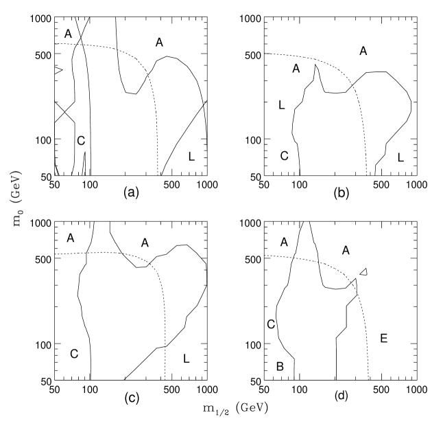
Figure 1: Contours of allowed parameter space. $m_{t}=170\hbox{\rm\,GeV}$ for each frame. In frame (a) $\tan\beta=5$, $\mbox{sgn}(\mu)=-$, and $A_{0}/m_{0}=0$, (b) $\tan\beta=5$, $\mbox{sgn}(\mu)=-$ and $A_{0}/m_{0}=-2$, in (c) $\tan\beta=20$, $\mbox{sgn}(\mu)=-$ and $A_{0}/m_{0}=3$, and in (d) $\tan\beta=10$, $\mbox{sgn}(\mu)=+$, and $A_{0}/m_{0}=-2$. See the text for explanation of letter labels.

The peak or spike in the allowed region for $m_{1/2}\simeq 130\hbox{\rm\,GeV}$ corresponds to $\chi\chi$ annihilations through a $Z$ pole. Since the LSP is not just a pure bino, and has some higgsino component to it, the $Z$ pole annihilation rate becomes extremely important in this region. Also, it appears obvious from the figures that the relic abundance constraint has the most effect in the increasing $m_{0}$ direction. This is understandable for several reasons. Away from the $Z$ and Higgs poles, the LSP annihilations occur most efficiently through the $t$-channel scalar diagrams. For a fixed $m_{\chi}$ value, which is roughly equivalent to fixed $m_{1/2}$, the annihilation cross-section decreases rapidly as the scalar mass $m_{0}$ increases. Hence, a cutoff in the allowed region must occur as $m_{0}$ increases.

Forays into the large $m_{1/2}$ region with $m_{0}$ fixed usually end up with other problems, the most common of which is $\tilde{l}_{R}$ becoming the LSP. This is simply a result of the renormalization group equation dependences on the $U(1)_{Y}$ couplings. A quick inspection of the renormalization group equations for $m_{\tilde{B}}$ and for $m_{\tilde{l}_{R}}$ proves that if $m_{1/2}\gg m_{0},m_{W}$, then the right-handed slepton must be lighter than the bino. Ruling out this region of parameter space can be considered a relic abundance constraint, since the dark matter probably cannot charged [17].

Realization that a weak-scale higgsino could be a legitimate dark matter particle is a rather recent development. One way to obtain an higgsino as the lightest neutralino is to make $|\mu|$ much less than the gaugino parameters in the neutralino mass matrix. A very low value of $\mu$ will create a roughly degenerate triplet of higgsinos. The charged higgsino and the neutral higgsinos can all coannihilate together with full $SU(2)$ strength, allowing the LSP to stay in thermal contact with the photons more effectively, thereby lowering the relic abundance of the higgsino LSP to an insignificant level. These coannihilation channels are often cited as the reason why higgsinos are not viable dark matter candidates. This claim is true in general, but there are two specific cases that I would like to summarize below that allow the higgsino to be a good dark matter candidate.

Drees et al. have pointed out that potentially large one-loop splittings among the higgsinos can render the coannihilations less relevant [18]. Under some conditions with light top squark masses, one-loop corrections to the neutralino mass matrix will split the otherwise degenerate higgsinos. If the mass difference can be more than about 5% of the LSP mass, then the LSP will decouple from the photons alone and not with its other higgsino partners, thereby increasing its relic abundance.

Another possibility [19] relating to a higgsino LSP is to set equal the bino and wino mass to approximately $m_{Z}$. Then set the $-\mu$ term to less than $m_{W}$. This non-universality among the gauginos and particular choice for the higgsino mass parameter, produces a light higgsino with mass approximately equal to $\mu$, a photino with mass at about $m_{Z}$, and the rest of the neutralinos and both charginos with mass above $m_{W}$. There are no coannihilation channels to worry about with this higgsino dark matter candidate since no other chargino or neutralino mass is near it. The value of $\tan\beta$ is also required to be near one so that the lightest neutralino is an almost pure symmetric combination of $\tilde{H}_{u}$ and $\tilde{H}_{d}$ higgsino states. The exactly symmetric combination does not couple to $Z$ boson (at tree level). The annihilation cross section near $\tan\beta\sim 1$ is proportional to $\cos^{2}2\beta$. The relic abundance scales inversely proportional to this, and so the nearly symmetric higgsino in this case is a very good dark matter candidate. Note that there are no $t$-channel slepton or squark diagrams since higgsinos couple to sfermions proportional to the fermion mass. Because the higgsino mass is below $m_{W}$, the top quark final state is kinematically inaccessible, and so the large top Yukawa cannot play a direct role in the higgsino annihilations.

This non-minimal higgsino dark matter candidate described in the previous paragraph was motivated by the $e^{+}e^{-}\gamma\gamma$ event reported by the CDF collaboration at Fermilab [20]. The non-minimal parameters [21] which leads to a radiative decay of the second lightest neutralino (photino) into the lightest neutralino (symmetric higgsino) and photon also miraculously yield a model with a good higgsino dark matter candidate.

5 Conclusion

The minimal model bino and the higgsino described above work as dark matter candidates both qualitatively and quantitatively. Nature, of course, might not conform to either of these specific possibilities, but it is straight-forward to catalog the non-minimal possibilities. There are, of course, numerous ways to go beyond what is presented here [22]. Scalar mass universality could be relaxed [23]. One could in fact suppose that $R$-parity is not exactly conserved and the LSP is not a stable particle. Perhaps one could allow small $R$-parity violations which create meta-stable LSPs whose lifetimes are greater than the age of the universe to solve the dark matter dilemma. However, it is not enough to just make the lifetime greater than the age of the universe. Remarkably, the measurements of positrons and photons in cosmic rays require that the LSP lifetimes into these particles be many orders of magnitude beyond the age of the universe [24]. In other words, it is not easy to make the LSP a meta-stable dark matter candidate. If $R$-parity were broken in nature, it appears necessary to look elsewhere for the dark matter candidate.

One common theme exists in non-minimal models which accommodate a supersymmetric solution to the dark matter problem. It is the requirement that $\chi\chi$ not couple to the $Z$ boson. A full strength $SU(2)$ coupling to the $Z$ boson generally allows too efficient LSP annihilation, and therefore too small relic abundance to be relevant to the dark matter problem. This theme can be found in several non-minimal examples such as the symmetric Higgsino [19, 18] described above, the $\tilde{Z}$ [25], and the sterile neutralino [26] dark matter candidates. Of course, the minimal model also provides a low-strength coupling to the $Z$ naturally with the mostly bino dark matter candidate [27]. The older supersymmetry dark matter literature considered the photino, which also does not couple to the $Z$, as the primary dark matter candidate [15].

Theoretical ideas about the low-energy superpartner spectrum always have dark matter implications. The supersymmetric solution to the dark matter problem is perhaps only superseded by gauge coupling unification in experimentally based indications that nature might be described by softly broken supersymmetry. It is mainly for this reason that much experimental effort is expended on the search for supersymmetric relics [28]. Likewise, theoretical efforts on understanding the origin of LSP stability and the prediction of dark matter properties should continue to enlighten us.

References

References

- [1] G. Farrar, P. Fayet, Phys. Lett. B 76, 575 (1978); S. Dimopoulos, H. Georgi, Nucl. Phys. B 193, 150 (1981); N. Sakai, T. Yanagida, Nucl. Phys. B 197, 83 (1982); S. Weinberg, Phys. Rev. D 26, 287 (1982).
- [2] T. Falk, K. Olive, M. Srednicki, Phys. Lett. B 339, 248 (1994).
- [3] E. Diehl, G.L. Kane, C. Kolda, J.D. Wells, Phys. Rev. D 52, 4223 (1995).
- [4] V. Trimble, Ann. Rev. Astron. Astrophys. 25, 425 (1987); P. Sikivie, Nucl. Phys. Proc. Suppl. 43, 90 (1995).
- [5] D. Schramm, M. Turner, astro-ph/9706069.
- [6] R. Wald, General Relativity, Chicago: University of Chicago Press (1984); E. Kolb, M. Turner, The Early Universe, Redwood City, USA: Addison-Wesley (1990).
- [7] B. Lee, S. Weinberg, Phys. Rev. Lett. 39, 165 (1977); M. Vysotskii, A. Dolgov, Ya. Zeldovich, Pisma Zh.Eksp.Teor.Fiz. 26, 200 (1977); P. Hut, Phys. Lett. B 69, 85 (1977).
- [8] K. Olive, D. Schramm, G. Steigman, Nucl. Phys. B 180, 497 (1981).
- [9] J. Ellis, J. Hagelin, D. Nanopoulos, M. Srednicki, Nucl. Phys. B 238, 453 (1984).
- [10] M. Srednicki, R. Watkins, K. Olive, Nucl. Phys. B 310, 693 (1988); P. Gondolo, G. Gelmini, Nucl. Phys. B 360, 145 (1991).
- [11] J.D. Wells, hep-ph/9404219; L. Roszkowski, Phys. Rev. D 50, 4842 (1994).
- [12] M. Drees, M. Nojiri, Phys. Rev. D 47, 376 (1993).
- [13] G. Kane, I. Kani, Nucl. Phys. B 277, 525 (1986).
- [14] K. Griest, D. Seckel, Phys. Rev. D 43, 3191 (1991).
- [15] H. Goldberg, Phys. Rev. Lett. 50, 1419 (1983).
- [16] G.L. Kane, C. Kolda, L. Roszkowski, J.D. Wells, Phys. Rev. D 49, 6173 (1994).
- [17] P. Smith, in Proceedings of the First International Symposium on Sources of Dark Matter in the Universe, edited by D. Cline, World Scientific, 1995. J. Basdevant, R. Mochkovitch, J. Rich, M. Spiro, A. Vidal-Madjar, Phys. Lett. B 234, 395 (1990).
- [18] M. Drees, M. Nojiri, D. Roy, Y. Yamada, Phys. Rev. D 56, 276 (1997).
- [19] G.L. Kane, J.D. Wells, Phys. Rev. Lett. 76, 4458 (1996); K. Freese, M. Kamionkowski, Phys. Rev. D 55, 1771 (1997).
- [20] S. Park, “Search for new phenomena at CDF,” 10th Topical Workshop on Proton-Antiproton Collider Physics, edited by Rajendran Raja and John Yoh, AIP Press, 1995.
- [21] S. Ambrosanio, G. Kane, G. Kribs, S. Martin, S. Mrenna, Phys. Rev. Lett. 76, 3498 (1996); Phys. Rev. D 55, 1372 (1997).
- [22] I do not discuss models of low-energy supersymmetry breaking which could have the gravitino as the LSP, or even exotic messenger particles as the cold dark matter. See for example, S. Dimopoulos, G. Giudice, A. Pomarol, Phys. Lett. B 389, 37 (1996).
- [23] P. Nath, R. Arnowitt, hep-ph/9701301.
- [24] J. Ellis, G. Gelmini, J. Lopez, D. Nanopoulos, S. Sakar, Nucl. Phys. B 373, 399 (1992); G. Kribs, I. Rothstein, Phys. Rev. D 55, 4435 (1997).
- [25] A. Gabutti, M. Olechowski, S. Cooper, S. Pokorski, L. Stodolsky, Astropart. Phys. 6, 1 (1996).
- [26] B. de Carlos, J.R. Espinosa, hep-ph/9705315.
- [27] L. Roszkowski, Phys. Lett. B 262, 59 (1991).
- [28] G. Jungman, M. Kamionkowski, K. Griest, Phys. Rept. 267, 195 (1996).