Constraints on Variant Axion Models

Abstract

A particular class of variant axion models with two higgs doublets and a singlet is studied. In these models the axion couples either to the $u$-quark or $t$-quark or both, but not to $b$, $c$, $s$, or $d$. When the axion couples to only one quark the models possess the desirable feature of having no domain wall problem, which makes them viable candidates for a cosmological axion string scenario. We calculate the axion couplings to leptons, photons and nucleons, and the astrophysical constraints on the axion decay constant $v_{a}$ are investigated and compared to the DFSZ axion model. We find that the most restrictive lower bound on $v_{a}$, that from SN1987a, is lowered by up to a factor of about 35, depending on the model and also the ratio of the vacuum expectation values of the higgs doublets. For scenarios with axionic strings, the allowed window for $v_{a}$ in the $u$ quark model can be more than two orders of magnitude. For inflationary scenarios, the cosmological upper bound on $v_{a}/N$, where $N$ is the QCD anomaly factor, is unaffected: however, the variant models have $N$ either 3 or 6 times smaller than the DFSZ model.

I Introduction

The relevance of instantons [3] to physics was first shown by ’t Hooft [4] in his resolution of the $U_{A}(1)$ problem [5]. It was first pointed out by him that the topological structure of the vacuum of any non-abelian gauge theory, which includes QCD, is non-trivial. There are gauge transformations, characterized by different topological numbers $n$ (the Pontryagin index), which can not be continuously deformed to one another. This gives rise to distinct ground states, labelled by different $n$ and separated by finite energy barriers. Instantons can be physically interpreted as quantum mechanical tunneling events, in Euclidean spacetime, between these different ground states [6, 7]. One then has to construct the true, gauge-invariant, vacuum out of these degenerate $n$-vacua by taking a linear combination

$$|\theta\rangle=\sum_{n}e^{-in\theta}|n\rangle.$$ (1)

In the path integral approach, the effect is to add the so-called $\theta$-term, to the ordinary QCD lagrangian, or

$${\mathcal{L}}_{\theta}=\theta{g_{s}^{2}\over 32\pi^{2}}G_{b}^{\mu\nu}{\tilde{G}_{b\mu\nu}}.$$ (2)

Under the combined action of charge conjugation and parity transformation the $\theta$-term changes sign and hence it violates CP invariance. There is also CP violation communicated from the quark mass matrix $M$: if we diagonalise it with a bi-unitary transformation, we find that the coupling constant $\theta$ is modified to

$$\bar{\theta}=\theta+\arg(\det M).$$ (3)

Despite being the coupling constant of a total derivative term, the parameter $\bar{\theta}$ is observable, through its effect on the neutron electric dipole moment [8]. The current experimental upper limit [9] on the electric dipole moment implies that $\bar{\theta}$ is less than about $10^{-9}$.

Such a small value of $\bar{\theta}$ contradicts our expectation that a dimensionless free parameter should be of order one. Many ideas have emerged in trying to resolve the puzzle. One of the most elegant solutions was proposed by Peccei and Quinn in 1977 [10]. The authors postulated the invariance of the lagrangian under the transformations of a new extra global chiral $U(1)$ symmetry, called PQ-symmetry, thus enlarging the symmetry group of the SM to $SU(3)_{C}\times SU(2)_{L}\times U(1)_{Y}\times U(1)_{PQ}$. To accomodate the extra charges of the new symmetry one needs (at least) one extra higgs doublet. When this symmetry is spontaneously broken, a pseudoscalar boson appears [11] in the theory, called the axion. Normally, one would think that the axion is massless, as it is the Nambu-Goldstone boson of the PQ symetry. However, the $U(1)_{PQ}$ symmetry is an anomalous one, spoiled by the effect of instantons in the QCD vacuum, and the axion picks up a small mass via the axion-gluon-gluon triangle anomaly.

The assignment of appropriate PQ-charges to the higgs fields and consequently to the quarks is responsible for the presence of the anomaly in the PQ current, and also for the variety of the axion models. In the original model, known as the PQWW (Peccei-Quinn-Weinberg-Wilczek) axion model [11], all the quarks of the same chirality were assigned the same PQ charge. Unfortunately the model was ruled out both by particle physics experiments and by astrophysical observations. The former gave constraints which came from $K,\ J/\psi$ and $\Upsilon$ meson decays, reactor and beam dump experiments and nuclear deexcitations [12]. The latter are in fact more restrictive and imply that $v_{a}>10^{10}$ GeV for most axion models considered to date [13]. A way out of this was first proposed by Kim in 1979 and subsequently by Shifman, Vainstein & Zakharov [14], who added a higgs singlet, thus enabling the axion decay constant to be much higher than the electroweak scale. However, it cannot be too high, as it is also possible to restrict $v_{a}$ from above through cosmological arguments. Coherent oscillations in axion field can be produced after inflation or via the formation of axionic cosmic strings. The requirement that the energy density in these oscillations is not large enough to overclose the universe puts an upper limit on $v_{a}$. The current values on these limits for the axion decay constant are $v_{a}$ less than about $10^{12}$GeV [15, 13] from inflationary scenarios and $v_{a}\lesssim 2.6\times 10^{11}$GeV [16] from axion strings (for $H_{0}=50$ km s^-1 Mpc^-1, and making the conservative assumption that radiation from infinite strings dominates that from loops). As we can see there is only a very small window left for the axion.

Cosmology also restricts on the value of $N$, the parameter that characterises the QCD anomaly, which is related to the number of quarks that couple to the axion. If there is no inflation between the PQ symmetry-breaking transition and the present day, a dense network of axion strings is formed. At around a temperature of 1 GeV, each string becomes the junction of (in our normalisation convention) $2N$ domain walls [17]. In order to avoid the domain walls dominating the energy density, $2N$ must be equal to unity, so that the string-wall system can annihilate. Models with $N>{1\over 2}$ must have a period of inflation at a low energy scale, or must reheat after inflation to less than the PQ symmetry-breaking temperature, to remain viable.

In this paper we examine some variant axion models based on those proposed first by Peccei, Wu & Yanagida [18] and independently by Krauss & Wilczek [19]. Their models were constructed with two higgs doublets and assigned of different PQ charges to different quarks. The original reason for this is that in order to make an axion model which avoided the particle physics constraints at the time it was essential to decrease the axion couplings to $c$ and $b$ quarks on one hand, and on the other to sufficiently suppress the $K^{+}\rightarrow\pi^{+}a$ decay rate. One must also have a sufficiently short lived axion so it cannot be detected by the other experiments. To accomplish that, one has to couple both the $c$ and $b$ quarks to the same higgs field. However, as we know the limits on the strangeness changing neutral currents are very tight and for that reason we have to couple the strange quark to the same higgs doublet as $c$ and $b$. Thus the only way to realise the Peccei-Quinn symmetry is to couple either the $u$ or the $t$ or both quarks to a second higgs doublet. So we have three different models in our hands, two of which have the cosmologically desirable property that $N={1\over 2}$, and hence have no domain wall problem.

Although the original models are also ruled out, along with the PQWW axion, by the astrophysical constraints, they also have extensions with a higgs singlet. The astrophysical constraints on these models, presented in the next section, have not previously been considered, and we present an analysis in this paper of the bounds on the axion scale that can be inferred from their couplings to electrons, photons, and nucleons in astrophysical processes. We find, as for the standard DFSZ [20] and KSVZ [14] invisible axions, that the tightest constraint comes, via the nucleon coupling, from SN1987a. However, in these variant models, the coupling is generally weaker, and weakens the lower bound on $v_{a}$ by a factor of between 1.4 and 35, depending on which quarks the axion couples to, and on the ratio of the vacuum expectation values of the higgs doublets. The cosmological upper bound on $v_{a}$ from the axion density is also reduced, by a factor of either 3 or 6, as a result of the smaller QCD anomaly factor.

II Description of the model

The models we are going to discuss were first proposed by Geng & Ng [21] and has elements from both the previously discussed one and that of DFSZ. There, an extra higgs singlet $\phi$ is introduced, the phase of which is reserved for the axion. A direct coupling of $\phi$ to quarks and leptons is impossible; but in the DFSZ model it couples to both $\phi_{1}$ and $\phi_{2}$. We however couple $\phi$ only to one of the two doublets, namely $\phi_{1}$, which then couples to the ‘special’ quarks according to the three models discussed above. The other higgs field couples to the rest of the quarks and the leptons. Therefore we have the following Yukawa interactions:

$${\mathcal{L}}_{Y} = f_{i1}^{u}(\bar{q}_{Li}\phi_{1}u_{R1})+f_{ij}^{d}(\bar{q}_{Li}\phi_{2}d_{Rj})+\sum_{j=2,3}f_{ij}^{u}(\bar{q}_{Li}\tilde{\phi}_{2}u_{Rj})+h.c.$$ (Model I)

$${\mathcal{L}}_{Y} = f_{i3}^{u}(\bar{q}_{Li}\phi_{1}u_{R3})+f_{ij}^{d}(\bar{q}_{Li}\phi_{2}d_{Rj})+\sum_{j=1,2}f_{ij}^{u}(\bar{q}_{Li}\tilde{\phi}_{2}u_{Rj})+h.c.$$ (Model II)

$${\mathcal{L}}_{Y} = f_{i1}^{u}(\bar{q}_{Li}\phi_{1}u_{R1})+f_{i3}^{u}(\bar{q}_{Li}\phi_{1}u_{R3})+f_{ij}^{d}(\bar{q}_{Li}\phi_{2}d_{Rj})+f_{i2}^{u}(\bar{q}_{Li}\tilde{\phi}_{2}u_{R2})+h.c.$$ (Model III)

where $\tilde{\phi}=i\sigma_{2}\phi^{*}$. Our nomenclature is the same as that of Peccei, Wu & Yanagida [18]. In the first model it is the $u$ quark that couples to the axion, whereas in the second is the $t$. Finally in the last model both quarks couple to the axion.

The most general renormalizable potential for the model, consistent with gauge, as well as PQ symmetry and renormalisability is [14, 21]

$$V = \lambda_{1}(\phi_{1}^{{\dagger}}\phi_{1}-v_{1}^{2}/2)^{2}+\lambda_{2}(\phi_{2}^{{\dagger}}\phi_{2}-v_{2}^{2}/2)^{2}+\lambda(\phi^{\ast}\phi-v^{2}/2)^{2}+$$ (5)

$$(a\phi_{1}^{{\dagger}}\phi_{1}+b\phi_{2}^{{\dagger}}\phi_{2})\phi^{\ast}\phi+c(\phi_{1}^{T}i\sigma_{2}\phi_{2}\phi^{2}+h.c)+d|\phi_{1}^{T}i\sigma_{2}\phi_{2}|^{2}+e|\phi_{1}^{{\dagger}}\phi_{2}|^{2}$$

The appropriate PQ transformations according to which the quarks acquire a PQ charge, as well as leaving the Yukawa lagrangians invariant are

$$q_{Rj} \longrightarrow e^{iQ_{Rj}\alpha}q_{Rj}$$ (6)

$$q_{Lj} \longrightarrow e^{iQ_{Lj}\alpha}q_{Lj}$$ (7)

$$\phi_{n} \longrightarrow e^{i(Q_{Lj}-Q_{Rj})\alpha}\phi_{n}$$ (8)

where $\alpha$ is explained below. In the models under discussion, we can choose an assignment of PQ charges such that $Q_{Lj}=0$ and only some of the $Q_{Rj}\neq 0$. Furthermore, we impose the normalisation condition that $Q_{Rj}=1$ for the ‘special’ quarks, which are $u_{R}$ and/or $t_{R}$. That further fixes the transformations for the higgs fields, which are as follows:

$$\langle\phi_{1}\rangle = {1\over\sqrt{2}}v_{1}\exp{[-i(\alpha+\alpha_{Z})]},$$ (9)

$$\langle\phi_{2}\rangle = {1\over\sqrt{2}}v_{2}\exp{(i\alpha_{Z})},$$ (10)

$$\langle\phi\rangle = {1\over\sqrt{2}}v\exp{(i\alpha)},$$ (11)

where $v_{1}$, $v_{2}$, $v$ are the vacuum expectation values of the higgs fields and $\alpha$, $\alpha_{Z}$ are the angles conjugate to the axion and the longitudinal degree of freedom of the $Z^{0}$ boson respectively.

Our following step is to find an expression for the axion decay constant. Let $a^{\prime}$ and $Z$ be the two goldstone bosons after the breaking of the Peccei-Quinn symmetry and before instanton effects are taken into consideration. The first one, $a^{\prime}$, is the massless axion and the second, $Z$, the goldstone boson that is eventually eaten by the $Z^{0}$. One then has the following equation

$$\left(\begin{array}[]{c}a^{\prime}\\ Z\end{array}\right)=\left(\begin{array}[]{lr}v_{a}&0\\ v_{10}&v_{11}\end{array}\right)\left(\begin{array}[]{c}\alpha\\ \alpha_{Z}\end{array}\right)$$ (12)

The $2\times 2$ matrix on the right hand side of (12) is the most general matrix compatible with the requirement not to mix the axion with the $Z^{0}$ boson. On the other hand if one takes the kinetic term for these massless scalar degrees of freedom then one has

$${1\over 2}[(\partial_{\mu}a^{\prime})^{2}+(\partial_{\mu}Z)^{2}] = {1\over 2}\{(v_{1}^{2}+v^{2})(\partial_{\mu}\alpha)^{2}+(v_{1}^{2}+v_{2}^{2})(\partial_{\mu}\alpha_{Z})^{2}$$ (14)

$$+v_{1}^{2}[(\partial_{\mu}\alpha)(\partial^{\mu}\alpha_{Z})+(\partial^{\mu}\alpha)(\partial_{\mu}\alpha_{Z})]\}.$$

The derivative of (12) compared with (14) gives the expression for the axion decay constant as well as the electroweak breaking scale

$$v_{a} = \sqrt{v^{2}+{{v_{1}^{2}v_{2}^{2}}\over{v_{1}^{2}+v_{2}^{2}}}},$$ (15)

$$v_{EW} = v_{11}=\sqrt{v_{1}^{2}+v_{2}^{2}}=\textrm{246 GeV},$$ (16)

$$v_{10} = {v_{1}^{2}\over{\sqrt{v_{1}^{2}+v_{2}^{2}}}}.$$ (17)

The expression is the same for all three models and as we can see, it is $v$ that ultimately fixes the scale for $v_{a}$.

On the other hand if we apply the same normalisation convention to the DFSZ axion, that is if we assign $Q_{Rj}=1$ to every quark, then the transformation of the higgs fields are:

$$\langle\phi_{1}\rangle = {1\over\sqrt{2}}v_{1}\exp{[-i(\alpha+\alpha_{Z})]},$$ (18)

$$\langle\phi_{2}\rangle = {1\over\sqrt{2}}v_{2}\exp{[i(-\alpha+\alpha_{Z})]},$$ (19)

$$\langle\phi\rangle = {1\over\sqrt{2}}v\exp{(i\alpha)},$$ (20)

where

$$v_{a} = \sqrt{v^{2}+{{4v_{1}^{2}v_{2}^{2}}\over{v_{1}^{2}+v_{2}^{2}}}},$$ (21)

$$v_{EW} = v_{11}=\sqrt{v_{1}^{2}+v_{2}^{2}}=\textrm{246 GeV},$$ (22)

$$v_{10} = {{v_{1}^{2}-v_{2}^{2}}\over{\sqrt{v_{1}^{2}+v_{2}^{2}}}}.$$ (23)

Our choice of charges ensure that $v_{a}$, which is essentially equal to the PQ symmetry-breaking scale, is also equal to the axion decay constant $f_{a}$ (as defined by Srednicki [23]). We have avoided using $f_{a}$ because of its many definitions in the literature.

III The axion couplings

Our next step is to determine the couplings of the axion to different quarks and leptons. In the basis where quarks $q^{\prime}_{j}$ are eigenstates of the weak interaction, the QCD part of the lagrangian is

$${\mathcal{L}}_{QCD}={\bar{q}^{\prime}_{j}}(i\gamma_{\mu}D^{\mu})q^{\prime}_{j}-{\bar{q}^{\prime}_{Li}}M_{ij}q^{\prime}_{Rj}-{\bar{q}^{\prime}_{Ri}}M^{{\dagger}}_{ij}q^{\prime}_{Lj}-{1\over 4}G_{b}^{\mu\nu}G_{b\mu\nu}+\theta{g_{s}^{2}\over 32\pi^{2}}G_{b}^{\mu\nu}\tilde{G}_{b\mu\nu},$$ (24)

where $M$ is the quark mass matrix, and depends on $\alpha$ and $\alpha_{Z}$, and hence $a^{\prime}$. If we diagonalise the quark mass matrix, we find that in the mass eigenstate basis the lagrangian is

$${\mathcal{L}}_{QCD} = {\bar{q}_{j}}(i\gamma_{\mu}D^{\mu}-m_{j})q_{j}-{1\over 4}G_{b}^{\mu\nu}G_{b\mu\nu}+{1\over 2}(\partial_{\mu}a^{\prime})^{2}+{g_{s}^{2}\over 32\pi^{2}}(\bar{\theta}-2N\frac{a^{\prime}}{v_{a}})G_{b}^{\mu\nu}\tilde{G}_{b\mu\nu}-$$ (26)

$$-{g_{j}\over 2v_{a}}\partial^{\mu}a^{\prime}\bar{q}_{j}\gamma_{\mu}\gamma_{5}q_{j},$$

where $N$ is explained below. If there were no mixing between the axion and the $Z^{0}$, the coupling $g_{j}$ would just be the difference of the PQ charges of the right and left-handed quarks $q_{j}$. The presence of the mixing modifies the relation to

$$g_{j}=(Q_{Rj}-Q_{Lj})-(Y_{Rj}-Y_{Lj}){v_{10}\over v_{11}},$$ (27)

where $Y_{Rj}$ and $Y_{Lj}$ are the hypercharges of the right and left chiral fields respectively of the $j$-th quark.

The constant $N$ depends on the number and type of particles with the gluon anomaly

$$N=\sum_{j}(Q_{Rj}-Q_{Lj})t_{j},$$ (28)

where $t_{j}$ is the index of the $SU(3)_{C}$ representation to which the fields belong (for the known quarks $t={1\over 2}$). Hence, in our normalisation convention, for Models I and II, $N={1\over 2}$, and for Model III, $N=1$. As advertised, the first two models have no axionic domain wall problem. In the case of the DFSZ axion we have $N=3$.

When calculating the axion-quark interactions in practice, the derivative interaction in (26) can prove troublesome, and it is usual to leave the phases corresponding to the axion degree of freedom in the quark mass matrix, so that the interaction term is

$${\mathcal{L}}_{aq}=-{m_{j}}\bar{q}_{j}e^{i\gamma_{5}(\Delta Q_{j}\alpha+\Delta Y_{j}\alpha_{z})}q_{j},$$ (29)

where $\Delta Q_{j}=Q_{Rj}-Q_{Lj}$ and $\Delta Y_{j}=Y_{Rj}-Y_{Lj}$. To first order in $a^{\prime}/v_{a}$, this gives

$${\mathcal{L}}_{aq}=-ig_{j}\frac{m_{j}}{v_{a}}a^{\prime}\bar{q}_{j}\gamma_{5}q_{j}.$$ (30)

The (pseudoscalar) Yukawa coupling of the interaction between the axion and the $j$-th quark is then clearly

$$h_{aj}=g_{j}{m_{j}\over v_{a}}.$$ (31)

The interactions with leptons can be calculated similarly. The term involving the axion and the $l$-th lepton $e_{l}$ is

$${\mathcal{L}}_{al}=-ig_{l}\frac{m_{l}}{v_{a}}a^{\prime}\bar{e}_{l}\gamma_{5}e_{l},$$ (32)

from which we define the Yukawa coupling

$$h_{al}=g_{l}{m_{l}\over v_{a}}.$$ (33)

It is useful for later calculations to express the couplings in terms of $\tan\beta$, where

$$\tan\beta\equiv{v_{2}\over v_{1}}.$$ (34)

So for Model I:

$$g_{u} = {v_{2}^{2}\over{v_{1}^{2}+v_{2}^{2}}}={\tan^{2}\beta\over{1+\tan^{2}\beta}}=\sin^{2}\beta,$$ (35)

$$g_{d_{j},e_{l}} = {v_{1}^{2}\over{v_{1}^{2}+v_{2}^{2}}}={1\over{1+\tan^{2}\beta}}=\cos^{2}\beta,$$ (36)

$$g_{c,t} = -{v_{1}^{2}\over{v_{1}^{2}+v_{2}^{2}}}=-{1\over{1+\tan^{2}\beta}}=-\cos^{2}\beta,$$ (37)

where $d_{j}=d,s,b$ and $e_{l}=e,\mu,\tau$. Using the same notation we can work out the couplings for Model II,

$$g_{u,c} = -{v_{1}^{2}\over{v_{1}^{2}+v_{2}^{2}}}=-{1\over{1+\tan^{2}\beta}}=-\cos^{2}\beta,$$ (38)

$$g_{d_{j},e_{l}} = {v_{1}^{2}\over{v_{1}^{2}+v_{2}^{2}}}={1\over{1+\tan^{2}\beta}}=\cos^{2}\beta,$$ (39)

$$g_{t} = {v_{2}^{2}\over{v_{1}^{2}+v_{2}^{2}}}={\tan^{2}\beta\over{1+\tan^{2}\beta}}=\sin^{2}\beta,$$ (40)

and for Model III:

$$g_{u,t} = {v_{2}^{2}\over{v_{1}^{2}+v_{2}^{2}}}={\tan^{2}\beta\over{1+\tan^{2}\beta}}=\sin^{2}\beta,$$ (41)

$$g_{d_{j},e_{l}} = {v_{1}^{2}\over{v_{1}^{2}+v_{2}^{2}}}={1\over{1+\tan^{2}\beta}}=\cos^{2}\beta,$$ (42)

$$g_{c} = -{v_{1}^{2}\over{v_{1}^{2}+v_{2}^{2}}}=-{1\over{1+\tan^{2}\beta}}=-\cos^{2}\beta.$$ (43)

Lastly, we write down the interaction between the axion and photons, which arises in the same way as for the axion-gluon interaction, through the $a\gamma\gamma$ triangle diagram

$${\mathcal{L}}_{a\gamma}=N_{e}{e^{2}\over 32\pi^{2}v_{a}}a^{\prime}F_{\mu\nu}\tilde{F}^{\mu\nu},$$ (44)

where

$$N_{e}=\sum_{j}(Q_{Rj}-Q_{Lj})e^{2}_{j}.$$ (45)

In this equation, $e_{j}$ is the electric charge of the $j$-th fermion (with each colour quark counted separately).

It is important to note that below the QCD scale ($\sim 200$MeV), free quarks do not exist so one has to consider the effective couplings of axions to nucleons, which arise from the axion mixing with $\pi^{0}$ and the $\eta^{\prime}$. It is exactly this mixing that allows us to calculate the axion mass and also has an effect on the coupling to two photons.

Standard current algebra techniques [22, 23] tell us that the physical axion $a$ has mass (including the strange quark)

$$m_{a}=\frac{m_{\pi}f_{\pi}}{v_{a}}N\left[\frac{z}{(1+z)(1+z+w)}\right]^{1/2},$$ (46)

and that its coupling to photons is

$${\mathcal{L}}_{a\gamma\gamma}={1\over 4}h_{a\gamma}aF\tilde{F},$$ (47)

where

$$h_{a\gamma}={e^{2}\over{4\pi^{2}}}\left[{1\over{v_{a}}}N\left({N_{e}\over N}-\frac{2(4+z+w)}{3(1+z+w)}\right)\right],$$ (48)

and we define $z$ and $w$ as [24]

$$z\equiv\frac{m_{u}}{m_{d}}=0.553\pm 0.043,$$

$$w\equiv\frac{m_{u}}{m_{s}}=0.029\pm 0.0043.$$

For models I & II one has $(N,N_{e})=(1/2,4/3)$ and for model III $(N,N_{e})=(1,8/3)$ . As we can see the ratio ${N_{e}/N}=8/3$ for all of them. This ratio holds both for the DFSZ and the KSVZ axion, as well as for GUT axion models based on SU(5) [23].

The same current algebra techniques enable us to compute the axion-nucleon coupling [23]. First we write down the anomaly-free axion current, including the strange quark

$$j^{a}_{\mu} = v_{a}\partial_{\mu}a+{1\over 2}\left(g_{u}-\frac{2}{1+z+w}N\right)\bar{u}\gamma_{\mu}\gamma_{5}u+{1\over 2}\left(g_{d}-\frac{2z}{1+z+w}N\right)\bar{d}\gamma_{\mu}\gamma_{5}d+$$ (50)

$$+{1\over 2}\left(g_{s}-\frac{2w}{1+z+w}N\right)\bar{s}\gamma_{\mu}\gamma_{5}s.$$

To find the couplings with the nucleons, we take the axionic current in the effective theory of nucleons,

$$j^{a}_{\mu}={1\over 2}\bar{\psi}(g_{0}+g_{3}\tau_{3})\gamma_{\mu}\gamma_{5}\psi,$$ (51)

where $\tau_{3}$ is the usual Pauli matrix, and $\psi$ is the nucleon doublet

$$\psi=\left(\begin{array}[]{c}p\\ n\end{array}\right),$$

sandwich it between nucleon states, and compare with the expression obtained by using Eq. (50). We find that the isoscalar and isovector couplings are given by

$$g_{0} = {1\over 6}(\Delta u+\Delta d-2\Delta s)\left(g_{u}+g_{d}-2g_{s}-\frac{1+z-2w}{1+z+w}2N\right)+$$ (53)

$$+{1\over 3}(\Delta u+\Delta d+\Delta s)(g_{u}+g_{d}+g_{s}-2N),$$

$$g_{3} = {1\over 2}(\Delta u-\Delta d)\left(g_{u}-g_{d}-\frac{1-z}{1+z+w}2N\right),$$ (54)

where $s_{\mu}\Delta q\equiv\langle\bar{\psi}|\bar{q}\gamma_{\mu}\gamma_{5}q|\psi\rangle$, with $s_{\mu}$ being the spin of the nucleon. We can find values for the $\Delta q$’s by combining the measurement of the proton spin structure function by the E143 collaboration [25], which gives $\Delta u+\Delta d+\Delta s=0.27\pm 0.10$, with quark model and SU(3) flavour symmetry predictions for nucleon and hyperon couplings. We find

$$\Delta u = 0.813\pm 0.072,$$ (55)

$$\Delta d = -0.444\pm 0.072,$$ (56)

$$\Delta s = -0.10\pm 0.04.$$ (57)

Translating these results into the language of the effective lagrangian approach we find

$${\mathcal{L}}_{a\bar{\psi}\psi}=-i{m_{\psi}\over v_{a}}a\bar{\psi}(g_{0}+g_{3}\tau_{3})\gamma_{5}\psi.$$ (58)

It is now straightforward to find the Yukawa couplings for the axion-proton and axion-neutron interactions. For Model I,

$$h_{ap} = \frac{m_{p}}{v_{a}}[-(0.678\pm 0.038)\cos 2\beta-(0.226\pm 0.058)],$$ (59)

$$h_{an} = \frac{m_{n}}{v_{a}}[(0.578\pm 0.038)\cos 2\beta+(0.136\pm 0.058)],$$ (60)

for Model II,

$$h_{ap} = \frac{m_{p}}{v_{a}}[-(0.678\pm 0.038)\cos 2\beta-(1.039\pm 0.058)],$$ (61)

$$h_{an} = \frac{m_{n}}{v_{a}}[(0.578\pm 0.038)\cos 2\beta+(0.579\pm 0.058)],$$ (62)

and Model III

$$h_{ap} = \frac{m_{p}}{v_{a}}[-(0.678\pm 0.038)\cos 2\beta-(0.587\pm 0.096)],$$ (63)

$$h_{an} = \frac{m_{n}}{v_{a}}[(0.578\pm 0.038)\cos 2\beta+(0.137\pm 0.096)].$$ (64)

Finally the Yukawa couplings for the DFSZ axion are

$$h_{ap} = \frac{m_{p}}{v_{a}}[-(1.357\pm 0.077)\cos 2\beta-(1.896\pm 0.275)],$$ (65)

$$h_{an} = \frac{m_{n}}{v_{a}}[(1.157\pm 0.077)\cos 2\beta+(0.276\pm 0.275)].$$ (66)

IV Astrophysical constraints

We are now interested in seeing how the astrophysical limits serve to constrain the couplings and hence the PQ scale $v_{a}$. In our case these constraints come exclusively from the application of energy loss arguments to stars [13]. According to it, if there are low mass particles like neutrinos or novel particles interacting weakly with matter and radiation like axions, they can be produced in large numbers in stellar interiors and can afterwards escape freely. In this way the stars are drained of energy and so alter their standard evolutionary course.

We can now proceed to the following step, which is checking how these three models behave under constraints coming from astrophysics. It would also be useful to compare the results with the DFSZ model, mainly for two reasons. First of all, it has significant similarities with our models, especially in the way that fermions acquire their PQ charges. Secondly, it is a well studied and established axion model and all existing constraints refer mostly to it.

We begin by estimating the bounds on the axion couplings to electrons. The most restrictive bound comes from the so called helium ignition argument in red giants [13, 26], which states that if a red giant produces a large number of neutrinos or other weakly interacting particles, then helium will ignite in a much later time because larger density will be required. For sufficiently light particles the energy loss rate would be so large, that helium would not ignite at all, so the stars would directly become white dwarfs. The limit is [26]

$$h_{ae}<2.5\times 10^{-13}.$$ (67)

So according to equations (33), (36), (39), (42) and (67) we get the following lower limit for the axion decay constant:

$$v_{a}>2\times 10^{9}\cos^{2}\beta\ \textrm{GeV},\\$$ (68)

which holds for all models. Another important interaction axions have is the one with photons. For the models under discussion it was first examined by Cheng, Geng & Ni [27]. The limit set on the constraint for the axion-photon coupling is [28]

$$h_{a\gamma}<1\times 10^{-11}.$$ (69)

From this and equation (24) is straightforward to conclude that

$$\hskip 113.81102ptv_{a}>8.5\times 10^{7}\ \textrm{GeV},\hskip 56.9055pt\textrm{(Models\ I, II)}\\$$ (70)

and

$$\hskip 102.43008ptv_{a}>1.7\times 10^{8}\ \textrm{GeV},\hskip 56.9055pt\textrm{(Model\ III)}\\$$ (71)

The strictest bound though arises from the axion coupling to nucleons. The most restrictive value for this constraint come from the supernova SN1987a neutrino signal [29]. The general argument underlying these kinds of measurements is as follows. We assume that we have some new light particles, produced in the interior of a neutron star, more weakly interacting than neutrinos e.g axions, and their Yukawa coupling noted as $h_{a\psi}$, where $\psi$ is the nucleon doublet. There are two possibilities. If $h_{a\psi}$ is too small, then axions cannot be trapped in the interior of the star. Their mean free path is bigger than the radius of the star and so they can escape freely. In this case axions are produced inside the whole volume of the star and so the axion flux would be $L_{a}\propto h_{a\psi}^{2}$. The reason for this is that axion production would be dominated by processes like axion bremsstrahlung from nucleons i.e $n+p\longrightarrow n+p+a$. Hence, $L_{a}$ increases with increasing $h_{a\psi}$ and eventually the axion flux equals the neutrino flux $L_{\nu}$. Let this value of the coupling be $h_{min}$. On the other hand, for larger $h_{a\psi}$, then axions can be trapped and thermalised, in which case they are emitted from a sphere of radius $R_{a}$. The stronger the coupling, the larger $R_{a}$ is. With blackbody surface emission, $L_{a}\propto R_{a}^{2}T^{4}(R_{a})$, where $T(R_{a})$ is the temperature at radius $R_{a}$. For a nascent neutron star, $R^{2}T^{4}(R)$ is a rapidly decreasing function of $R$. We require that $L_{a}<L_{\nu}$, and thus $R_{a}>R_{\nu}$: thus there is a value of $h_{a\psi}$, say $h_{max}$, above which the axion flux drops below the neutrino flux again. Hence the range $h_{min}<h_{a\psi}<h_{max}$ is excluded because the axion flux would dominate the one coming from the neutrinos. If one is to remain conservative, many body effects should be taken into account, in which case the limit from this constraint is [30]

$$(h_{ap}^{2}+2h_{an}^{2})^{1/2}<2.85\times 10^{-10}.$$ (72)

This constraint puts bounds on $v_{a}$, which we write as

$$v_{a}>(0.33\times 10^{10})(A\cos^{2}2\beta+B\cos 2\beta+C)^{1/2}\ \mathrm{GeV}.$$ (73)

The values of $A$, $B$ and $C$, and their uncertainties (which arise from the uncertainties in $\Delta q$, $z$, and $w$) are displayed in Table 1.

For completeness, we also give the bounds on the DFSZ model originating from the electron and photon couplings:

$$v_{a} > 4\times 10^{9}\cos^{2}\beta\ \textrm{GeV},$$ (74)

$$v_{a} > 5.1\times 10^{8}\ \textrm{GeV},$$ (75)

It is clear that the lower bound on the axion scale from the red giant constraint (which operates on the axion-electron coupling) is relaxed by a factor of about 2. The axion-photon coupling depends on $v_{a}/N$, as does the mass of the axion and the cosmological constraint in inflationary scenarios (in the axion string scenario, $N=1/2$). These particular constraints on the ratio $v_{a}/N$, are therefore the same for our variant axion models as for DFSZ.

On the other hand, it is not so straightforward to compare the nucleon constraints. For one to see how these bounds affect $v_{a}$, we plot graphs of $v_{a}$ against $\beta$ for every model including the DFSZ. One can easily check from (Fig. 1) that the lower bound is shifted downwards by a factor of 1.4–35 compared to that of the DFSZ axion. We have also displayed how the uncertainties in the nucloeon couplings are propagated into uncertainties in the bounds.

V Conclusions

Although the axion solution to the strong CP problem is one of the most physically appealing, axions themselves face a great problem. Despite the fact that they interact very weakly with matter and so are very difficult to track, particle physics experiments together with astrophysical considerations and cosmology have managed to constrain axion models significantly. In this paper we have found the constraints on for axion models with non-standard couplings to quarks and leptons, using data from E143 to determine the values of the nucleon couplings, which provide the strongest constraint. We find that the bounds are generally weakened, as the nucleon couplings in our variant axion models are smaller. The most spectacular effect is for Model I near $\beta\sim\pi/4$: the bound dips to about $v_{a}>2\times 10^{8}$ GeV, about a factor 35 less than the DFSZ value. Models I and II have the desirable feature that the QCD anomaly coefficient $N={1\over 2}$, which means that they have no domain wall problem, and therefore are viable models for an axion string scenario. For Model I, the lower bound on $v_{a}$ can dip to $2\times 10^{8}$ GeV for values of $\beta$ near $\pi/4$. Recalling the upper bound on $v_{a}$ in the axion string scenario, $v_{a}<2.6\times 10^{11}$ GeV for $H_{0}=50$ km s^-1 Mpc^-1 [16], we see that the ‘window’ for this axion string scenario is actually quite large.

In an inflationary scenario, the cosmological upper bound is on $v_{a}/N$, and so the upper bound on $v_{a}$ itself is reduced by a factor of 6 for Models I and II, and a factor 3 for Model III.

Model	$A$	$B$	$C$
I	$1.13\pm 0.14$	$0.62\pm 0.18$	$0.09\pm 0.06$
II	$1.13\pm 0.14$	$2.75\pm 0.31$	$1.75\pm 0.26$
III	$1.13\pm 0.14$	$1.11\pm 0.31$	$0.38\pm 0.17$
DFSZ	$4.52\pm 0.14$	$6.42\pm 1.76$	$3.75\pm 1.35$

TABLE I.: Table of values of coefficients in Eq. (73), with experminetal uncertainties, for the three variant axion models considered, compared with the values for the canonical DFSZ model.

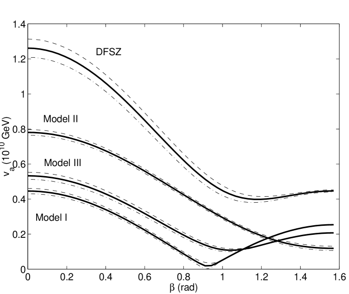
FIG. 1.: The lower bound on the Peccei-Quinn symmetry-breaking scale $v_{a}$ for variant axion models described in the text and the DFSZ model, plotted as a function of $\beta$. Here, $\tan\beta=v_{2}/v_{1}$, where $v_{1}$ and $v_{2}$ are the vacuum expectation values of the two higgs fields giving masses to the fermions. The dashed and dot-dashed lines indicate the uncertainties arising from the nucleon couplings.