DESY 97-117 TUM/T39-97-17 HUB-EP-97/33

A lattice determination of the second moment of the
polarised valence quark distribution

M. Göckeler^a, R. Horsley^b, L. Mankiewicz^c, H. Perlt^d, P.Rakow^e,

G. Schierholz^e,f and A. Schiller^d

^a Institut für Theoretische Physik, Universität Regensburg,

D-93040 Regensburg, Germany

^b Institut für Physik, Humboldt-Universität zu Berlin,

Invalidenstrasse 110, D-10115 Berlin, Germany

^c Institut für Theoretische Physik, TU München, Germany

^d Institut für Theoretische Physik, Universität Leipzig,

D-04109 Leipzig, Germany

^e Deutsches Elektron-Synchrotron DESY,

Institut für Hochenergiephysik und HLRZ,

D-15735 Zeuthen, Germany

^f Deutsches Elektron-Synchrotron DESY,

D-22603 Hamburg, Germany

Abstract:
We perform a Monte Carlo calculation of the second moment of the polarised valence quark distributions in the nucleon, using quenched Wilson fermions. The special feature of this moment is that it is directly accessible experimentally. At a scale of $\mu\approx 2\,\mbox{GeV}$ we find $\Delta^{(1)}u=0.198(8)$, $\Delta^{(1)}d=-0.0477(33)$. We compare these numbers with recent experimental results of the SMC collaboration.

Measurements of polarised deep inelastic structure functions of the nucleon have revealed that only a small fraction of the nucleon’s spin is carried by the spin of the quarks [1, 2, 3, 4, 5]. This raises the question as to how the spin of the nucleon is distributed among spin and orbital angular momentum of its constituents. The constituents are valence quarks, sea quarks and gluons. In this paper we shall be concerned with the spin carried by the valence quarks.

In the naive quark parton model the unpolarised structure functions and the polarised structure function $g_{1}$ can be expressed in terms of the probability distributions for finding a quark with spin parallel, $q_{\uparrow}$, and antiparallel, $q_{\downarrow}$, to the longitudinally polarised nucleon:

$$F_{1}(x) = \frac{1}{2}\sum_{q}e_{q}^{2}[q(x)+\bar{q}(x)],$$ (1)

$$g_{1}(x) = \frac{1}{2}\sum_{q}e_{q}^{2}[\Delta q(x)+\Delta\bar{q}(x)],$$ (2)

where

$$q(x)=q_{\uparrow}(x)+q_{\downarrow}(x),\;\;\Delta q(x)=q_{\uparrow}(x)-q_{\downarrow}(x).$$ (3)

By analogy one can define hadron inclusive structure functions

$$F_{1}^{h}(x,z) = \frac{1}{2}\sum_{q}e_{q}^{2}[q(x)D_{q}^{h}(z)+\bar{q}(x)D_{\bar{q}}^{h}(z)],$$ (4)

$$g_{1}^{h}(x,z) = \frac{1}{2}\sum_{q}e_{q}^{2}[\Delta q(x)D_{q}^{h}(z)+\Delta\bar{q}(x)D_{\bar{q}}^{h}(z)],$$ (5)

where $D_{q}^{h}(z)$ is the fragmentation function for quark $q$ to produce hadron $h$, and $z=p^{h}\cdot p/p\cdot q$ with $p^{h}$, $p$ and $q$ being the hadron, nucleon and photon momentum, respectively. Of interest to us is the polarisation asymmetry [6]

$$A^{h}=\frac{g_{1}^{h}(x,z)}{F_{1}^{h}(x,z)}.$$ (6)

Consider the polarisation asymmetry of $\pi^{+}$ minus $\pi^{-}$ inclusive cross sections. For a proton and deuteron target we find

$$A_{p}^{\pi^{+}-\pi^{-}}=\frac{4\Delta u^{\rm val}(x)-\Delta d^{\rm val}(x)}{4u^{\rm val}(x)-d^{\rm val}(x)}$$ (7)

and

$$A_{d}^{\pi^{+}-\pi^{-}}=\frac{\Delta u^{\rm val}(x)+\Delta d^{\rm val}(x)}{u^{\rm val}(x)+d^{\rm val}(x)},$$ (8)

respectively. Note that the fragmentation functions drop out completely and that the sea quarks do not contribute. This happens because of isospin invariance relating the various fragmentation functions with each other. The advantage of these quantities is that they allow a direct measurement of the valence quark distribution functions [6]. The latter can then be compared with the results of quenched lattice calculations [7].

The polarisation asymmetries (7), (8) have been measured by the SMC collaboration. For the first moment

$$\Delta q=\int_{0}^{1}dx\Delta q(x),\;q=u,d\;$$ (9)

it has been found, [8], $\Delta u^{\rm val}=1.01\pm 0.19\pm 0.14$ and $\Delta d^{\rm val}=-0.57\pm 0.22\pm 0.11$. The lattice results are, [9], $\Delta u=0.841(52)$ and $\Delta d=-0.245(15)$, which include data on $24^{3}32$ lattices. The analysis has recently been extended to the second moment

$$\Delta^{(1)}q=\int_{0}^{1}dxx\Delta q(x).$$ (10)

The SMC collaboration has obtained results for $\Delta^{(1)}u$ and $\Delta^{(1)}d$ [10]. A similar analysis will be published soon by the HERMES collaboration, [11].

In QCD, $\Delta^{(1)}q=\mbox{\small$\frac{1}{2}$}a_{1}^{(q)}$ where $a_{1}^{(q)}$ is the matrix element of the operator

$${\cal O}_{5}^{({\cal M})\mu\nu}=\left({i\over 2}\right)\overline{q}\gamma^{({\cal M})\mu}\gamma^{({\cal M})5}\stackrel{{\scriptstyle\leftrightarrow}}{{D}}^{({\cal M})\nu}q,$$ (11)

defined by

$$\langle\vec{p},s|{\cal S}{\cal O}_{5}^{({\cal M})\mu\nu}|\vec{p},s\rangle=a_{1}^{(q)}{\cal S}s^{({\cal M})\mu}p^{({\cal M})\nu},$$ (12)

where ${\cal S}$ symmetrises and subtracts traces. We have emphasised Minkowski space with an index ${\cal M}$. $s^{({\cal M})}$ is the nucleon spin vector defined by

$$s^{({\cal M})}=\left({\vec{s}\cdot\vec{p}\over E},\vec{s}\right),\qquad\vec{s}=\sigma m\left(\vec{e}+{\vec{p}\cdot\vec{e}\over m(E+m)}\vec{p}\right),$$ (13)

with $\vec{e}$ being the rest frame quantisation axis and $\sigma=\pm 1$ the spin component along this axis. We now euclideanise and discretise the operator given in eq. (11). Let us first define our euclidean operator by

$${\cal O}_{5\mu\nu}=\mbox{\small$\frac{1}{2}$}\overline{q}\gamma_{\mu}\gamma_{5}\stackrel{{\scriptstyle\leftrightarrow}}{{D}}_{\nu}q.$$ (14)

Its transcription to the lattice is straightforward. However on the lattice the symmetry group is reduced from $O(4)$ to the hypercubic group $H(4)$. This loss of symmetry increases the possibilities of mixing under renormalisation. In the continuum, application of ${\cal S}$ is sufficient to construct operators which are multiplicatively renormalisable (in the flavour-nonsinglet sector).

${\cal O}(a)$		$\langle\vec{p},s|{\cal O}^{R}|\vec{p},s\rangle$	Representation
${\cal O}_{5\{\mu\nu\}}$	$1\leq\mu<\nu\leq 4$	$-a_{1}s_{\{\mu}p_{\nu\}}$	$\tau_{1}^{(6)}$, ${\cal C}=-1$
${\cal O}_{5,ii}-\mbox{\small$\frac{1}{4}$}\sum_{\lambda}{\cal O}_{5,\lambda\lambda}$	$1\leq i\leq 3$	$-a_{1}s_{i}p_{i}$	$\tau_{4}^{(3)}$, ${\cal C}=-1$

Table 1: Multiplicatively renormalisable lattice operators ${\cal O}(a)$ and the continuum matrix elements of the corresponding renormalised operators. $\{\cdots\}$ means symmetrisation. $\tau_{n}^{(m)}$ denotes the representation, [13], with $m$ being its dimension. ${\cal C}$ is the charge conjugation eigenvalue of the operator.

To achieve the same on the lattice one has to work slightly harder [13]. In our case one finds two multiplets of operators (corresponding to two inequivalent irreducible representations of $H(4)$) which are multiplicatively renormalisable. They are given in table 1. For each of them we obtain the renormalised operator ${\cal O}^{R}(\mu)$ (renormalisation scale $\mu$) from the lattice operator ${\cal O}(a)$ (lattice constant $a$) by multiplying with the appropriate renormalisation factor $Z_{\cal O}$:

$${\cal O}^{R}(\mu)=Z_{\cal O}((a\mu)^{2},g(a)){\cal O}(a).$$ (15)

In our computation we have only considered $\vec{p}=\vec{0}$ or $\vec{p}=\vec{p}_{1}\equiv p_{1}\vec{e}_{1}$ together with spin-quantisation axis $\vec{e}=\vec{e}_{2}$. Thus from Table 1 we can consider

$${\cal O}_{a_{1},a} = {\cal O}_{5\{12\}},$$

$${\cal O}_{a_{1},b} = {\cal O}_{5\{42\}}.$$ (16)

Note that for a non-zero matrix element for ${\cal O}_{a_{1},a}$ we must have a non-zero three-momentum, while for ${\cal O}_{a_{1},b}$ we do not have this restriction. As including three-momentum in the matrix element makes the signal more noisy we would expect the best result to come from using zero three-momentum together with the matrix element of ${\cal O}_{a_{1},b}$.

The nucleon matrix elements are computed from ratios of three- to two- point functions. Thus with

$$C_{\Gamma}(t,\vec{p}) = \sum_{\alpha\beta}\Gamma_{\beta\alpha}\langle B_{\alpha}(t,\vec{p})\overline{B}_{\beta}(0,\vec{p})\rangle,$$

$$C_{\Gamma}(t,\tau;\vec{p},{\cal O}_{a_{1}}) = \sum_{\alpha\beta}\Gamma_{\beta\alpha}\langle B_{\alpha}(t,\vec{p}){\cal O}_{a_{1}}(\tau)\overline{B}_{\beta}(0,\vec{p})\rangle,$$ (17)

and

$$R(t,\tau;\vec{p},{\cal O}_{a_{1}})={C_{\mbox{\small$\frac{1}{2}$}(1+\gamma_{4})i\gamma_{5}\gamma_{2}}(t,\tau;\vec{p},{\cal O}_{a_{1}})\over C_{\mbox{\small$\frac{1}{2}$}(1+\gamma_{4})}(t;\vec{p})},$$ (18)

we find

$$R(t,\tau;\vec{p},{\cal O}_{a_{1},a}) = -{1\over Z_{{\cal O}_{a_{1}}}}{1\over 2\kappa}{1\over 4}{m_{N}\over E_{N}}p_{1}a_{1}\qquad t\gg\tau\gg 0,$$

$$R(t,\tau;\vec{p},{\cal O}_{a_{1},b}) = -{1\over Z_{{\cal O}_{a_{1}}}}{1\over 2\kappa}{i\over 4}m_{N}a_{1}\qquad t\gg\tau\gg 0,$$ (19)

where $\kappa$ is the Wilson hopping parameter and $m_{N}$ ($E_{N}$) is the mass (energy) of the nucleon. Eq. 19 holds provided the operator is inserted at a Euclidean time $\tau$ sufficiently far away from the nucleon source at time $t=0$ and the sink at time $t$. We then expect to observe a ‘plateau’ where $R$ is independent of $\tau$.

We have simulated quenched Wilson fermions with five different $\kappa$ values on $N_{s}^{3}\times 32$ lattices with $N_{s}=16$, $N_{s}=24$ at $\beta\equiv 6/g^{2}=6.0$. $p_{1}$ is taken to be the lowest possible momentum, namely $p_{1}=2\pi/N_{s}$. More details of the computation may be found in ref. [7]. Note, in particular, that we have dropped the quark-line disconnected terms. This, coupled with the use of the quenched approximation, means that sea quarks play only a small role in our calculation, so that we are effectively measuring valence moments only. The masses for this calculation are taken from [15]. In Fig. 1

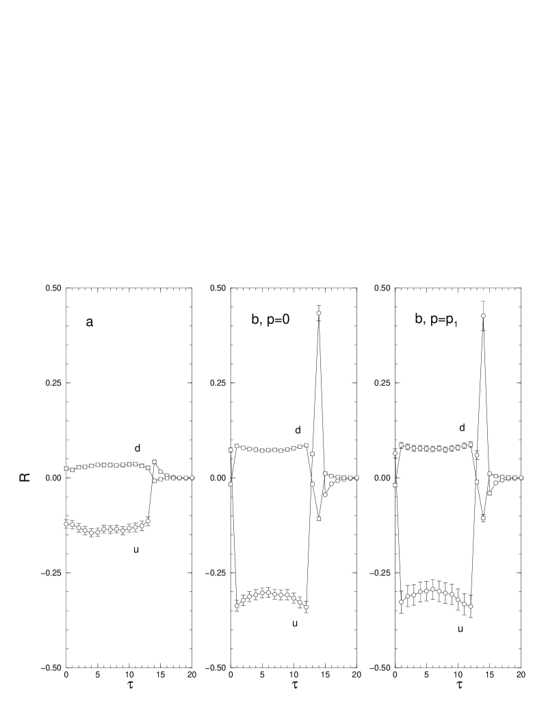
Figure 1: The $R\equiv R(t=13,\tau,\vec{p},{\cal O}_{a_{1}})$ ratio at $\kappa=0.1530$.

we show typical ratios for $t=13$. The fit interval for the determination of the plateau is chosen to lie between $\tau=4$ and $\tau=9$. These values of $\tau$ seem to be sufficiently far away from both the baryon source $t=0$ and sink $t=13$ to avoid contamination with excited states.

To find $\Delta^{(1)}u$ and $\Delta^{(1)}d$, we must also calculate the renormalisation constant $Z_{{\cal O}_{a_{1}}}^{\overline{MS}}$. This was given in ref. [12] where it was called $Z_{{\cal O}_{r_{2a}}}$, see also [17]. Explicitly, we have

$$Z^{\overline{MS}}_{{\cal O}_{a_{1}}}((a\mu)^{2},g)=1-{g^{2}\over 16\pi^{2}}C_{F}\left[\gamma_{{\cal O}_{a_{1}}}\ln(a\mu)+B_{{\cal O}_{a_{1}}}^{\overline{MS}}\right]+O(g^{4}),$$ (20)

with $C_{F}={4\over 3},\gamma_{{\cal O}_{a_{1}}}={16\over 3}$, and $B_{{\cal O}_{a_{1}}}^{\overline{MS}}=0.3454$. We shall work, for convenience, at a scale of $\mu=1/a$. This gives for $\beta=6.0$, $Z_{{\cal O}_{a_{1}}}(1,1)=0.997$. We see that the $O(g^{2})$ coefficient is thus very small. This is because ‘tadpole terms’ in the perturbation expansion have cancelled. Indeed if we try to improve the result using ‘tadpole improved boosted perturbation theory’, [18], we find

$$Z^{\overline{MS}}_{{\cal O}_{a_{1}}}((a\mu)^{2},g))={u_{0}\over u_{0}^{n_{D}}}\left(1-{\alpha^{\overline{MS}}(\mu)\over 4\pi}C_{F}[\gamma_{{\cal O}_{a_{1}}}\ln(a\mu)+B_{{\cal O}_{a_{1}}}^{\overline{MS}}+(n_{D}-1)\pi^{2}]\right),$$ (21)

where $n_{D}$ is the number of derivatives, $u_{0}=\langle\mbox{\small$\frac{1}{3}$}\mbox{tr}U_{\Box}\rangle^{\mbox{\small$\frac{1}{4}$}}$ with $U_{\Box}$ the expectation value of the plaquette, and $\alpha^{\overline{MS}}(\mu)$ is used here as the boosted coupling. In our case $n_{D}=1$, so the coefficient of the coupling constant is unchanged and remains small, and at $\beta=6.0$, $\alpha^{\overline{MS}}(1/a)\approx 0.1981$, [18], so that

$$Z_{{\cal O}_{a_{1}}}^{\overline{MS}}(1,1)=0.993$$ (22)

which is a negligible change in the previous result. Our conclusion is that the uncertainty in the renormalisation constants is probably quite small, although only a full non-perturbative calculation would reveal this of course. We shall use, in the following, the result from eq. (22).

Finally we note that to determine the scale $\mu$ for our results we must first estimate $a$. Measuring a physical quantity on the lattice (such as a mass) and comparing this to the experimental value determines $a$. However as Wilson fermions have $O(a)$ corrections, it is better to set the scale from a gluonic quantity, as this has only $O(a^{2})$ corrections. This also avoids the need of making a chiral extrapolation in the masses. From the string tension $K$ we get (using a scale of $\sqrt{K}=427\mbox{MeV}$, [19])

$$a^{-1}=1.95(2)\,\mbox{GeV},$$ (23)

where the error is purely statistical.

We now come to our results. In Tables 2, 3

$\kappa$	$0.1515$	$0.1530$	$0.1550$
# configs	$O(400)$	$O(500)$	$O(900)$
$\Delta^{(1)}_{a}u|_{\vec{p}=\vec{p}_{1}}$	0.236(13)	0.240(15)	0.219(26)
$\Delta^{(1)}_{b}u|_{\vec{p}=\vec{0}}$	0.241(10)	0.234(9)	0.223(10)
$\Delta^{(1)}_{b}u|_{\vec{p}=\vec{p}_{1}}$	0.244(18)	0.229(19)	0.233(24)
$\Delta^{(1)}_{a}d|_{\vec{p}=\vec{p}_{1}}$	-0.0577(52)	-0.0577(60)	-0.0549(148)
$\Delta^{(1)}_{b}d|_{\vec{p}=\vec{0}}$	-0.0596(27)	-0.0559(24)	-0.0556(38)
$\Delta^{(1)}_{b}d|_{\vec{p}=\vec{p}_{1}}$	-0.0596(48)	-0.0586(51)	-0.0651(10)

Table 2: The results for $\Delta^{(1)}q$ on a $16^{3}\times 32$ lattice.

$\kappa$	$0.1550$	$0.1558$	$0.1563$
# configs	$O(100)$	$O(100)$	$O(100)$
$\Delta^{(1)}_{a}u|_{\vec{p}=\vec{p}_{1}}$	0.200(25)	0.172(32)	0.122(58)
$\Delta^{(1)}_{b}u|_{\vec{p}=\vec{0}}$	0.219(14)	0.211(14)	0.193(17)
$\Delta^{(1)}_{b}u|_{\vec{p}=\vec{p}_{1}}$	0.223(21)	0.212(25)	0.184(37)
$\Delta^{(1)}_{a}d|_{\vec{p}=\vec{p}_{1}}$	-0.0437(81)	-0.0409(141)	-0.0755(293)
$\Delta^{(1)}_{b}d|_{\vec{p}=\vec{0}}$	-0.0526(48)	-0.0463(68)	-0.0416(103)
$\Delta^{(1)}_{b}d|_{\vec{p}=\vec{p}_{1}}$	-0.0559(63)	-0.0473(95)	-0.0344(195)

Table 3: The results for $\Delta^{(1)}q$ on a $24^{3}\times 32$ lattice.

we give our numbers and in Fig. 2

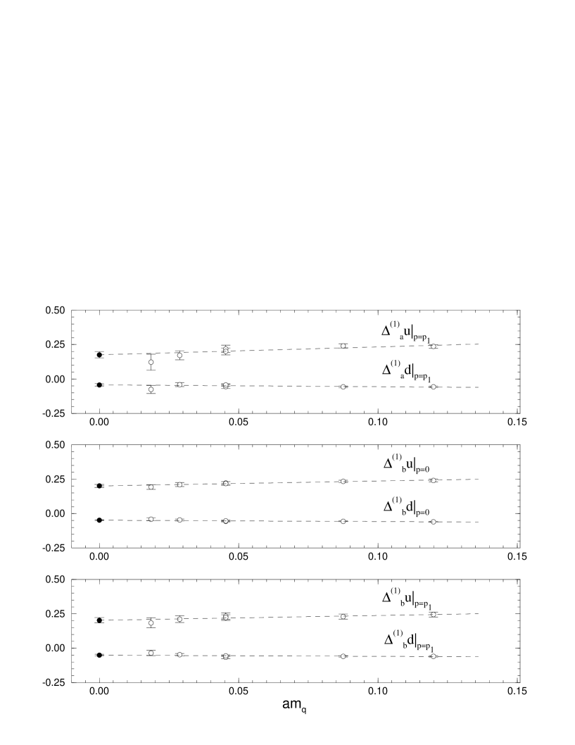
Figure 2: The chiral extrapolation for $\Delta^{(1)}q$.

we plot $\Delta^{(1)}u$, $\Delta^{(1)}d$ against the bare quark mass

$$am_{q}={1\over 2}\left({1\over\kappa}-{1\over\kappa_{c}}\right),$$ (24)

together with a linear chiral extrapolation. (The chiral limit is determined from the vanishing of the pion mass, which occurs here at $\kappa_{c}=0.15721(1)$, [15]. We roughly estimate our quark masses from $am_{q}^{R}=Z_{m}am_{q}\sim 1.21am_{q}$, [15], to be $m^{\overline{MS}}(2\,\mbox{GeV})\sim 290$, $210$, $110$, $70$, $45$ MeV.) The quality of the data seems quite good. The statistics for the light quark masses is rather low, so although we include them in the linear fit, they should be regarded as only confirming the heavier quark mass results. Note that the results for $\kappa=0.1550$ have been measured on two different lattice sizes and differ by less than their errors which would indicate that at least up to this value of $\kappa$ finite size effects are under control. At each $\kappa$ we have three different measurements of $\Delta^{(1)}q$, one at $\vec{p}=\vec{0}$ and two at $\vec{p}=\vec{p}_{1}$. If Lorentz invariance has been restored, all three measurements should agree, which is what they do within errors. As expected the $\vec{p}=0$ results are the best, although the other signals are quite acceptable. It would also seem that the gradient in the chiral extrapolation is rather small over this quark mass range. The values in the chiral limit are given in Table 4.

$\Delta^{(1)}_{a}u|_{\vec{p}=\vec{p}_{1}}$	$\Delta^{(1)}_{b}u|_{\vec{p}=\vec{0}}$	$\Delta^{(1)}_{b}u|_{\vec{p}=\vec{p}_{1}}$	$\Delta^{(1)}_{a}d|_{\vec{p}=\vec{p}_{1}}$	$\Delta^{(1)}_{b}d|_{\vec{p}=\vec{0}}$	$\Delta^{(1)}_{b}d|_{\vec{p}=\vec{p}_{1}}$
0.176(23)	0.201(10)	0.203(20)	-0.0427(94)	-0.0477(41)	-0.0507(71)

Table 4: The results for $\Delta^{(1)}q$ in the chiral limit.

For definiteness, averaging the three different measurements we quote a result of

$$\Delta^{(1)}u = 0.198(8),$$

$$\Delta^{(1)}d = -0.0477(33),$$ (25)

at a scale of $\mu^{2}\approx 4$ GeV².

We first compare our result with that given in [20] where a phenomenological fit was made from the experimental data for the polarised structure function $g_{1}$ to obtain the polarised parton distribution functions. Taking the second moment of their $NLO$ fit functions yields values of around $\Delta^{(1)}u\approx 0.15$, $\Delta^{(1)}d\approx-0.055$, at a scale of $\mu^{2}=4$ GeV². While the $d$ moment is in agreement with our result, their $u$ moment is a little smaller than ours.

We can see how the matrix element runs with the scale upon using the renormalisation group equation

$$\Delta^{(1)}q(\mu^{\prime})=\left({\alpha_{\overline{MS}}(\mu^{\prime})\over\alpha_{\overline{MS}}(\mu)}\right)^{C_{F}{\gamma_{{\cal O}_{a_{1}}}\over 2b_{0}}}\Delta^{(1)}q(\mu),$$ (26)

with the value of $\alpha^{\overline{MS}}(2\mbox{GeV})\approx 0.1981$, [18], and with $b_{0}=11-\mbox{\small$\frac{2}{3}$}n_{f}=11$, as we are working in the quenched approximation. Thus at $\mu^{2}=10\mbox{GeV}^{2}$ we find:

$$\Delta^{(1)}u = 0.189\pm 0.008,$$

$$\Delta^{(1)}d = -0.0455\pm 0.0032.$$ (27)

No great dependence on the scale is seen.

Finally our predictions can now be compared with the preliminary results of the SMC collaboration [10] at the scale $\mu^{2}=10$ GeV² which read:

$$\Delta^{(1)}u = 0.169\pm 0.018\pm 0.012,$$

$$\Delta^{(1)}d = -0.055\pm 0.027\pm 0.011,$$ (28)

where the first quoted error is statistical and the second one systematic. The integrals have been evaluated using data from the measured range $0.003\leq x\leq 0.7$. The unmeasured regions below $x=0.003$ and above $x=0.7$ give probably a negligible contribution to $\Delta^{(1)}u$ and $\Delta^{(1)}d$. The lattice and experimental results agree within their respective errors.

References

-
[1]
M.J. Alguard et al., Phys. Rev. Lett. 37, 1258 (1976);
ibid 37, 1261 (1976);
G. Baum et al., Phys. Rev. Lett. 51, 1135 (1983). -
[2]
J. Ashman et al., Phys. Lett. B206, 364 (1988);
J. Ashman et al., Nucl. Phys. B238, 1 (1989). -
[3]
B. Adeva et al., Phys. Lett. B302, 500 (1993);
ibid B320, 400 (1994);
D. Adams et al., Phys. Lett. B329, 399 (1994); ibid B357, 248 (1995). - [4] P. L. Anthony et al., Phys. Rev. Lett. 71, 959 (1993).
-
[5]
K. Abe et al., Phys. Rev. Lett. 74, 346 (1995); ibid
75, 25 (1995);
K. Abe et al., Phys. Lett. B364, 61 (1995). - [6] L. L. Frankfurt, M. I. Strikman, L. Mankiewicz, A. Schäfer, E. Rondio, A. Sandacz and V. Papavassiliou, Phys. Lett. B230, 141 (1989).
- [7] M. Göckeler, R. Horsley, E.-M. Ilgenfritz, H. Perlt, P. Rakow, G. Schierholz and A. Schiller, Phys. Rev. D53, 2317 (1996).
- [8] B. Adeva et al., Phys. Lett. B369, 93 (1996).
- [9] C. Best, M. Göckeler, R. Horsley, L. Mankiewicz, H. Perlt, P. Rakow, A. Schäfer, G. Schierholz and S. Schramm, preprint DESY 97-116 (1997) (hep-ph/9706502), to appear in the proceedings of DIS97.
- [10] J. Pretz, Dissertation, Mainz (1997).
- [11] M. Düren, private communication.
- [12] C. Best, M. Göckeler, R. Horsley, E.-M. Ilgenfritz, H. Perlt, P. Rakow, A. Schäfer, G. Schierholz and S. Schramm, preprint DESY 97-41 (1997) (hep-lat/9703014), to appear in Phys. Rev. D.
- [13] M. Göckeler, R. Horsley, E.-M. Ilgenfritz, H. Perlt, P. Rakow, G. Schierholz and A. Schiller, Phys. Rev. D54, 5705 (1996).
- [14] M. Göckeler, R. Horsley, H. Perlt, P. Rakow, G. Schierholz, A. Schiller and P. Stephenson, Phys. Lett. B391, 388 (1997).
- [15] M. Göckeler, R. Horsley, H. Perlt, P. Rakow, G. Schierholz, A. Schiller and P. Stephenson, preprint DESY 97-125, HUB-EP-97/38 (1997) (hep-lat/9707021).
- [16] M. Göckeler, R. Horsley, E.-M. Ilgenfritz, H. Perlt, P. Rakow, G. Schierholz and A. Schiller, Nucl. Phys. B472, 309 (1996).
- [17] M. Göckeler et al., in preparation.
- [18] G. P. Lepage and P. B. Mackenzie, Phys. Rev. D48, 2250 (1993).
- [19] E. Eichten, K. Gottfried, T. Kinoshita, K. D. Lane and T. M. Yan, Phys. Rev. D21, 203 (1980).
- [20] T. Gehrmann and W. J. Stirling, Phys. Rev. D53, 6100 (1996).