JLAB-TH-97-30
Meson Decays In A Quark Model
W. Robertsa and B. Silvestre-Bracb
a Department of Physics, Old Dominion University
Norfolk, VA 23529 USA
and
Thomas Jefferson National Accelerator Facility
12000 Jefferson Avenue, Newport News, VA 23606, USA
b Institut des Sciences Nucléaires,
53 avenue des Martyrs, Grenoble, France
A recent model of hadron states is extended to include meson decays. We find that the overall success of the model is quite good. Possible improvements to the model are suggested.
I Introduction and Motivation
Recently, a model for the description of hadronic states has been developed and applied to both meson and baryon spectra [1, 2]. The success of the model in describing the spectra in these sectors has led to attempts to take the model further by applying it to multiquark states [3]. This success has also led to the question of whether the model describes other aspects of baryon and meson spectroscopy adequately. In particular, it is useful to know whether the model can help shed light on some of the many outstanding puzzles in hadron spectroscopy. Before such a question can be addressed, the model should be able to reproduce those portions of hadron phenomenology that are better understood. In this article, we present the results of application of the wave functions obtained from this model to the strong decays of light mesons. We find that the model is as successful as other models, for the decays examined.
The rest of this article is organized as follows. In the next section we summarize the salient points of the hadronic model, as well as the model we use to describe the decays of hadrons. In section 3 we present our results with some discussion, while our conclusions are presented in section 4.
II The Model
Two ingredients are essential for a good description of meson decays. One of these is a realistic description of the mesons themselves. The second is a valid description of the transition operator. Both of these depend very much on our educated guesses about non-perturbative QCD dynamics. In the case of the former, there are many models proposed. We confine ourselves to the work of [1]. For the meson decays, there are also a number of models proposed, but we will limit ourselves to the pair creation model first proposed by Micu [4], and popularized by the Orsay group [5].
A Spectrum
One possibility for the analysis of the meson spectrum is the use of a ‘good’ quark-antiquark potential. This is the course we pursue. Although the one-gluon exchange mechanism suggests possible functional forms for some terms of the potential, the fact that we still do not know much about the mechanism of confinement means that we must rely on phenomenology to determine both the form and the parameters of the potential. Several potentials have been proposed in the past in the literature. We believe that in models of the kind that we propose, a very crucial test is a unified description of the meson and baryon spectra. This has been undertaken by one of us [1, 2], and six different potentials have been found which fulfill this criterion. These potentials have been applied, not only to the meson and baryon sectors, but also to tetra-quark states [3], as well as to a description of the interaction [6]. The results in all of these cases have been encouraging.
In this paper, we select two of these potentials for this study. The general form of each potential has been more or less imposed by some basic QCD constraints, but the parameters have been determined by a fit to a well-chosen sample of meson and baryon states. Both potentials are used with a non-relativistic kinetic energy term, and they take the general form
| (1) |
One peculiarity of these potentials is that the range of the hyperfine term is mass dependent through the relation
| (2) |
In the limit of a vanishing range, this term gives the usual Fermi-Breit prescription .
These potentials contain neither spin-orbit nor tensor contributions so that states have the same wave functions. In the same spirit, and mixings are absent. This approximation can have some effect on the results, but we are mainly interested in the gross features of the decays, so that the potentials are quite satisfactory from this point of view. Furthermore, there is no isospin dependence (this is a property shared by most potential models: in [7], isospin dependence is introduced by means of mixing through annihilation). Thus, the and , as well as the and resonances are degenerate, both in energy and in wave function. More dramatic is the case of the pseudoscalar mesons, as this leads to a degeneracy of the and the non-strange part of the . Isospin dependence appears only through the flavor part of the wave function, although there probably should be a difference in the spatial part of the wave function as well. In any case, we consider two potentials that yield good overall results for the meson spectrum.
The first potential, denoted AL1, has the usual Coulomb+linear form for the central part, and its parameters are
The second choice of potential, denoted AP1, has a confining term suggested by the Regge trajectory behavior of orbital states in a non-relativistic treatment. The parameters are
Both potentials reproduce spectra of comparable quality and are simple enough to be handled without any difficulty. In particular, it is quite easy to solve the differential equation resulting from the Schrödinger equation. However, the radial part of the meson wave function is calculated numerically on a grid. Such a form is not easily used for studying more complicated problems: a continuous expression is usually more convenient.
| system | masses (MeV) | ||||
|---|---|---|---|---|---|
| experiment | exact | ||||
| 138 | 138 | 194 | 140 | 138 | |
| 1300 | 1303 | - | 1314 | 1303 | |
| 769 | 770 | 771 | 770 | 770 | |
| 782 | 770 | 771 | 770 | 770 | |
| K | 496 | 490 | 532 | 492 | 491 |
| K∗ | 893 | 903 | 906 | 904 | 903 |
| 1019 | 1020 | 1025 | 1021 | 1020 | |
| aJ | 1251 | 1208 | 1210 | 1208 | 1208 |
| fJ | 1245 | 1208 | 1210 | 1208 | 1208 |
To solve this problem, we approximate the regularized part of the exact radial wave function by a linear combination of gaussian functions,
| (3) |
For a given number of gaussian functions, the parameters and are determined by a variational procedure on the energy of the considered state. is a rather rough approximation, but or greatly improves the results. This is illustrated in figure 1, where the exact wave function, as well as the approximations, are plotted for the pion, for a large range of values. In this figure, the curves on the left are for the potential AL1, while those on the right are for AP1. We see that except for very short distances, the approximation with 3 gaussian terms gives essentially the exact wave function. This expression, eqn. (3), is then used in our model for meson decays.

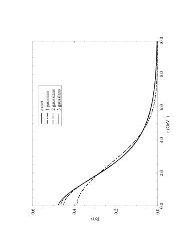
We show in table I a few of the masses obtained in this way, for the potential Al1. Experimental values are shown in the second column, while the exact predictions are given in the third. The masses obtained using the expansion of the wave function in gaussian functions are shown in the next three columns for , respectively. We see that the approximation with gives essentially the same results as the exact case, confirming the trend illustrated in figure 1.
B Decays
For the OZI [8] allowed decays of a meson, we assume that quark pair creation, somewhere within the volume of the parent hadron, provides the dominant contribution. In fact, for the operator we choose, this creation can take place anywhere in space, but the wave function overlaps ensure that the dominant contribution to the amplitude comes from creation within the ‘confines’ of the parent hadron.
The full mechanism for strong decays is, of course, as yet unknown, but the success of pair creation models hints at what may be the most important aspects of the underlying dynamics. We assume that the operator responsible for the decay is
| (4) | |||||
| (5) |
Here, and are the color and flavor wave functions of the created pair, both assumed to be singlet, is the spin triplet wave function of the pair, and is the vector harmonic indicating that the pair is in a relative P-wave. creates a quark, and creates an antiquark.
For the transition , we are interested in evaluating the transition amplitude , given by
| (6) |
The details of this calculation are given elsewhere [9, 10]. Once is evaluated, we calculate the decay rate as
| (7) |
where is the phase space for the decay. We have investigated three possible choices for this phase space. The first choice is that of fully relativistic phase space, for which
| (8) |
with , and is calculated in the rest frame of the parent meson. The second choice is fully non-relativistic phase space, with
| (9) |
Our third choice is the ‘weak-binding’ phase space suggested by Kokoski and Isgur [11], for which
| (10) |
where the ’s are effective meson masses (in the model) without hyperfine interaction. For the , we use the values suggested in [11].
III Results and Discussion
We have performed a number of fits to the experimental data; we show the results of these fits in table II. In addition, using the parameters obtained from these fits, we have calculated the amplitudes for a number of other decays. These are presented in tables III, IV and V. In table II, we consider only decays in which the daughter mesons are narrow. For this purpose, we treat the as a narrow state. In tables III to V, we extend the calculation to include ’s and ’s as daughter mesons.
| decay | (MeV1/2) | |||||||
|---|---|---|---|---|---|---|---|---|
| Fit I | Fit II | Fit III | Fit IV | Fit V | Fit VI | Fit VII | experiment | |
| 12.3 | 11.1 | 10.4 | 12.1 0.3 | 12.0 0.3 | 12.2 0.3 | |||
| 8.6 | 7.8 | 7.2 | 7.5 0.2 | 7.7 0.2 | 7.5 0.2 | |||
| 2.8 | 2.5 | 2.3 | 2.3 0.1 | 2.4 0.1 | 2.3 0.1 | |||
| 9.5 | 8.6 | 9.2 | 8.4 0.3 | 9.2 0.3 | 9.4 0.2 | |||
| 2.5 | 2.3 | 2.3 | 1.4 0.1 | 1.6 0.1 | 1.4 0.0 | |||
| 0.7 | 0.8 | 0.7 | 0.3 0.0 | 0.4 0.0 | 0.3 0.0 | |||
| 11.5 | 10.5 | 5.5 | 19.6 1.6 | 17.2 1.6 | 16.5 0.4 | |||
| 9.5 | 8.6 | 6.3 | 9.6 0.4 | 9.7 0.3 | 8.7 0.2 | |||
| 2.0 | 1.8 | 2.0 | 1.5 0.1 | 1.4 0.1 | 1.6 0.0 | |||
| 4.2 | 3.8 | 3.9 | 2.6 0.2 | 2.6 0.1 | 2.7 0.1 | |||
| 9.4 | 8.5 | 8.1 | 7.5 0.2 | 8.3 0.3 | 8.1 0.2 | |||
| 2.6 | 2.4 | 2.4 | 1.9 0.1 | 2.1 0.1 | 2.1 0.1 | |||
| 7.2 | 6.5 | 5.5 | 5.4 0.1 | 5.3 0.1 | 4.8 0.1 | |||
| 1.9 | 1.7 | 1.4 | 1.7 0.0 | 1.6 0.0 | 1.5 0.0 | |||
| 1.3 | 1.2 | 0.1 | 1.3 0.1 | 2.6 0.3 | 1.9 0.0 | |||
| 7.5 | 6.8 | 3.3 | 12.5 1.0 | 11.1 1.0 | 10.3 0.3 | |||
| 7.8 | 7.1 | 7.3 | 6.8 0.2 | 6.7 0.2 | 7.4 0.2 | |||
| 2.1 | 1.9 | 1.8 | 1.1 0.1 | 1.2 0.1 | 1.1 0.0 | |||
| 4.2 | 3.6 | 4.0 | 2.7 0.2 | 2.5 0.2 | 2.7 0.1 | |||
| 3.5 | 3.2 | 1.5 | 4.9 0.4 | 5.0 0.3 | 3.9 0.1 | |||
| 4.8 | 4.3 | 5.1 | 4.6 0.2 | 3.7 0.2 | 5.3 0.1 | |||
| 3.0 | 2.7 | 3.3 | 2.0 0.2 | 1.4 0.2 | 2.2 0.1 | |||
The numbers in column two (Fit I) of these tables result from a fit to the amplitude for , using the usual form of the operator. The numbers in column three (Fit II) result from using the same operator, but fitting to the 22 decays shown in table II. Column four (Fit III) corresponds to a similar global fit, but using a modified transition operator. In this case, the operator has been modified by making the change
| (11) | |||
| (12) |
with , and . For the results of column 2 and 3, we find and , respectively. These three fits all result from the AL1 wavefunctions, expanded to .
The effects of the size of the expansion basis of the wave functions are illustrated in Fits IV and V; the former is a one parameter global fit () using the AL1 wave functions with three gaussians, while the latter uses the same wave functions with the modified transition operator (, , ). Fits VI and VII show the effects of a change in potential. Both of these arise from the AP1 wave functions in conjunction with the modified transition operator: Fit VI uses wave functions with a single gaussian (, , ), while the wave functions of Fit VII are expanded in a basis of three gaussians (, , ). For Fits III, V, VI and VII, the theoretical errors are evaluated using the covariance matrix resulting from the fit. All of the amplitudes are calculated using the weak-binding prescription for phase space. As can be seen from tables II, there are few instances in which a change of the choice of potential or wave function expansion, accompanied by apparently radical changes in fit parameters, induces a big change in the amplitude. In particular, the modification of the operator induces an enhancement of large decay amplitudes, while keeping the others at approximately constant values, thus increasing the agreement with the experimental data. The most noticeably different fit is Fit IV.
The effective of modifying the wave function is less obvious, although the wave functions expanded on a larger basis () gives slightly better fits than those expanded on the smaller basis.
We have also fitted using only the first three decays of table II, namely , and . We have also omitted various ones of the decays in table II from the fit, such as the decays of the . Except for a very few isolated amplitudes, none of these modifications have had a significant effect on the decay amplitudes that result. We note also that non-relativistic phase space consistently gives by far the worst results, while the weak-binding prescription gives the best results. However, we find that in the case of the full relativistic phase space, there are two decays that consistently contribute the most to the ‘badness of fit’. One is the decay , while the other is . But for these two decays, relativistic phase space and the weak-binding prescription would give fits with essentially the same values of .
The wave functions that we use take into account SU(3) breaking effects. Strictly speaking we should also fully include such effects in the amplitudes. These effects arise from three sources. The most obvious of these is in the calculation of phase space, where we use either the physical masses of the states (for non-relativistic and relativistic phase space), or the ‘weak-binding’ masses appropriate to the mesons in the decay. The second source of SU(3) breaking is due to the fact that the amplitude depends on the momentum of the daughter mesons, calculated in the rest frame of the parent. Here we also use the physical masses of the states to calculate this momentum. The third source of SU(3) breaking arises in the evaluation of the matrix element of the transition operator. The masses of the quarks or, more precisely, various ratios of masses of the quarks, enter explicitly into this calculation. We have found that treating the , and as degenerate provides the best results. Thus, SU(3) breaking at this level is not necessary.
A few comments on the results of table II are in order. The amplitudes for the and are calculated from those for the and states of the model spectrum, assuming a mixing angle of . In tables III to V, we ignore this mixing and present results for the unmixed and . The and are assumed to be
| (13) |
respectively. The is assumed to be purely , and the is taken as pure . Finally, in all of the results we have ignored mixings of the type , while in tables III to V, we have also ignored mixings of the type .
The numbers in table II show that the model reproduces the experimental data reasonably well, for all of the scenarios presented. Not surprisingly, the three-parameter fits are somewhat better than any of the one-parameter fits. With few exceptions, amplitudes that are found to be large experimentally, also turn out to be large in the model, and the same is generally true of small amplitudes. The few exceptions where a large discrepancy exists are , and . In the case of the first of these decays, we note simply that the status of this state is very much in question, so that the partial widths themselves are also uncertain. In the case of the , we note that the mixing we have used has not resulted from a ‘rigorous’ calculation, but is simply ‘borrowed’ from the literature. In the case of the , there is the possibility of mixing with the radially excited state, not taken into account in this calculation. However, indications are that this mixing is very small [7], and would probably not play a large role in bringing the model calculation into closer agreement with the experimental measurement.
| decay | (MeV1/2) | ||||
|---|---|---|---|---|---|
| Fit I | Fit II | Fit III | experiment | ||
| 9.3 1.0 | 8.4 0.9 | 9.1 1.2 | dominant a | ||
| 3.1 0.7 | 2.8 0.6 | 2.1 0.5 | |||
| 0.3 0.3 | 0.3 0.2 | 0.2 0.2 | possibly seen | ||
| 4.2 0.2 | 3.8 0.1 | 3.0 0.1 | |||
| 2.0 0.1 | 1.8 0.1 | 1.7 0.1 | |||
| 0.5 0.1 | 0.4 0.0 | 0.3 0.0 | 0.9 0.1 | ||
| 5.2 0.1 | 4.7 0.1 | 3.7 0.1 | 10.5 0.4 | ||
| 0.6 0.0 | 0.5 0.0 | 0.4 0.0 | — | ||
| 0.1 0.0 | 0.1 0.0 | 0.1 0.0 | — | ||
| 0.1 0.0 | 0.1 0.0 | 0.1 0.0 | — | ||
| 11.2 1.9 | 10.1 1.8 | 9.4 2.1 | seen | ||
| 0.4 0.7 | 0.4 0.7 | 0.3 0.5 | — | ||
| 0.5 2.0 | 0.4 1.8 | 0.3 1.3 | — | ||
| 3.8 0.3 | 3.4 0.2 | 3.4 0.2 | seen | ||
| 0.5 0.2 | 0.4 0.2 | 0.3 0.1 | — | ||
| 2.2 0.2 | 1.9 0.1 | 2.0 0.0 | — | ||
| 1.4 0.2 | 1.3 0.1 | 0.8 0.1 | — | ||
| 0.1 0.0 | 0.1 0.0 | 0.0 0.0 | — | ||
| 2.8 0.9 | 2.5 0.8 | 1.4 0.5 | — | ||
| 4.6 0.2 | 4.1 0.2 | 5.5 0.2 | 8.6 0.8 a | ||
| 7.9 0.2 | 7.1 0.2 | 5.6 0.3 | |||
| 2.9 0.4 | 2.6 0.3 | 2.1 0.3 | — | ||
| 1.4 0.3 | 1.3 0.2 | 0.7 0.2 | |||
| 3.5 0.4 | 3.1 0.4 | 3.0 0.5 | 3.2 0.6 a | ||
| 2.1 0.5 | 1.9 0.5 | 1.0 0.3 | |||
In tables III to V, we have extended the model calculation to examine decays of a few, semi-randomly selected, radially and orbitally excited states. For these tables, the results correspond to the first three fits of II, respectively. We preface our discussion here by reminding the reader that the assignment of many of the experimentally observed states is still not clear, and it is not our aim, at least not in this work, to clarify the assignments of any of these states, but simply to see how well our model for their decays (and implicitly, of their spectrum) works. Thus, we have chosen only a few of the ‘better established’ states for this discussion. Note that if the predicted value for an amplitude is less than 0.05 MeV1/2, we do not show the amplitude.
In obtaining the numbers for decays with a broad vector meson ( or ; the is less than 10 MeV wide, and we treat it as a narrow state in our calculation) in the final state, we integrate over the line shape of the broad final state. That is, for such decays, the decay rate is taken as
| (14) |
where denotes the vector meson, and is the total width of the vector meson. The errors on the theoretical numbers in these tables arise from evaluating the amplitudes at the upper and lower limits of the mass ranges allowed by the experimental error on the masses of the states.
As with the fitted decays, we find that the overall agreement of the model predictions with the experimental data is quite good. There are a few instances in which there is noticeable disagreement, and we comment on these below.
Our results for the are ‘consistent’ with experiment, in that the decay of this state to is ‘dominant’ (of a total width of about 400 MeV), while we predict a partial width of about 100 MeV. Not many other exclusive final states have been identified in the decays of this meson, leaving the possibility that much of its width comes from decays to excited mesons (or exotics). For the rest of the decays of the states, the results that we obtain are in reasonable agreement with what little data there is.
| decay | (MeV1/2) | ||||
|---|---|---|---|---|---|
| Fit I | Fit II | Fit III | experiment | ||
| 9.5 0.1 | 8.6 0.1 | 8.7 0.2 | |||
| 2.5 0.1 | 2.3 0.1 | 1.7 0.1 | |||
| 0.7 0.1 | 0.8 0.1 | 0.4 0.1 | |||
| 0.5 0.1 | 0.4 0.1 | 0.4 0.1 | not seen | ||
| 11.6 5.7 | 10.5 5.1 | 15.6 6.6 | |||
| 9.5 3.6 | 8.6 3.2 | 10.3 2.5 | |||
| 6.1 6.1 | 5.5 5.5 | 6.2 6.2 | seen | ||
| 9.4 0.2 | 8.5 0.2 | 8.4 0.2 | |||
| 2.6 0.1 | 2.4 0.1 | 2.3 0.1 | |||
| 0.0 0.1 | 0.0 0.1 | 0.0 0.0 | — | ||
| 3.2 0.5 | 2.9 0.5 | 2.2 0.4 | — | ||
| 9.4 0.5 | 8.5 0.4 | 8.5 0.5 | seen b | ||
| 1.9 0.3 | 1.7 0.3 | 1.3 0.2 | |||
| 12.6 0.3 | 11.4 0.3 | 15.5 0.3 | — | ||
| 7.3 0.1 | 6.6 0.1 | 8.5 0.1 | seen | ||
| 0.0 3.9 | 0.0 3.6 | 0.0 3.6 | seen | ||
| 5.6 0.2 | 5.0 0.2 | 6.8 0.1 | seen | ||
| 1.5 0.1 | 1.4 0.1 | 1.8 0.0 | — | ||
| 1.4 1.4 | 1.2 1.2 | 0.8 0.8 | — | ||
| 12.6 1.9 | 11.4 1.7 | 11.2 2.0 | dominant | ||
In the channels, our predictions are in quite good agreement with experiment, except for the decays of the . However, the assignment of this state is so uncertain, (e. g.; there still is the question of whether this is a single state or not) that interpretation of the discrepancy is difficult. In this sector there is one decay that is worthy of some comment. At its nominal mass, the will not decay to , yet the partial width for this decay has been listed as ‘large (dominant)’ [13]. However, we see that if we change the mass of this state by 10 MeV in our model (a small amount, considering how broad states are expected to be), the amplitude for decay to grows rapidly. This is not surprising, as this is an -wave amplitude, which grows roughly as , where is the mass of parent and is the threshold for the decay. This would suggest that either (a) this state is more massive than reported in [12]; or (b) the amplitude grows so rapidly that we should integrate over the line-shape of at least the in calculating the amplitude. This decay also illustrates some of the importance of threshold effects.
| decay | (MeV1/2) | ||||
|---|---|---|---|---|---|
| Fit I | Fit II | Fit III | experiment | ||
| 0.0 2.9 | 0.0 2.6 | 0.0 2.2 | c d | ||
| 3.0 0.3 | 2.7 0.3 | 2.5 0.3 | 6.1 1.1 | ||
| 0.9 0.1 | 0.8 0.1 | 0.6 0.1 | |||
| 4.7 0.1 | 4.2 0.1 | 4.2 0.1 | 3.8 1.0 | ||
| 1.8 0.1 | 1.6 0.1 | 1.1 0.1 | |||
| 6.9 0.1 | 6.2 0.1 | 6.1 0.0 | |||
| 1.3 0.1 | 1.2 0.1 | 0.7 0.1 | |||
| 8.5 0.2 | 7.7 0.2 | 7.7 0.3 | 2.3 1.2 | ||
| 2.4 0.2 | 2.2 0.2 | 1.6 0.1 | |||
| 10.3 0.1 | 9.3 0.1 | 10.5 0.2 | 12.8 0.9 | ||
| 4.5 0.2 | 4.1 0.2 | 3.1 0.2 | |||
| 1.3 0.1 | 1.2 0.1 | 1.1 0.0 | b | ||
| 0.1 0.0 | 0.1 0.0 | 0.8 0.0 | — | ||
| 2.8 0.1 | 2.5 0.1 | 1.5 0.1 | — | ||
| 3.8 0.1 | 3.4 0.1 | 2.3 0.1 | 4.0 b | ||
| 4.9 0.1 | 4.4 0.0 | 3.3 0.1 | 9.5 b | ||
| 7.5 0.2 | 6.8 0.2 | 10.4 0.3 | |||
| 11.2 0.1 | 10.2 0.1 | 13.2 0.1 | — | ||
| 7.9 0.1 | 7.1 0.1 | 7.1 0.2 | |||
| 4.2 0.1 | 3.7 0.1 | 3.1 0.1 | 0.4 0.4 | ||
| 2.1 0.2 | 1.9 0.2 | 1.3 0.1 | |||
| 3.7 0.2 | 3.3 0.2 | 2.5 0.2 | 3.1 0.2 | ||
| 6.4 0.1 | 5.8 0.1 | 4.4 0.1 | 5.2 0.3 | ||
| 5.8 0.7 | 5.2 0.6 | 4.1 0.6 | — | ||
| 8.7 0.8 | 7.8 0.7 | 6.6 0.8 | 5.8 | ||
| 12.2 0.9 | 11.0 0.8 | 10.1 0.5 | 10.1 | ||
| 2.4 0.2 | 2.2 0.2 | 2.1 0.5 | — | ||
| 1.5 0.9 | 1.3 0.8 | 0.6 0.7 | |||
| 4.4 1.5 | 4.0 1.3 | 4.0 1.6 | — | ||
| 3.1 1.7 | 2.8 1.5 | 1.6 1.0 | |||
| 3.0 0.5 | 2.7 0.4 | 2.8 0.9 | seen b | ||
| 2.3 2.0 | 2.1 1.8 | 1.2 1.5 | |||
| 0.0 0.8 | 0.0 0.7 | 0.0 0.4 | — | ||
| 0.0 0.1 | 0.0 0.1 | 0.0 0.0 | |||
| 3.6 0.1 | 3.2 0.1 | 5.2 0.1 | |||
| 4.0 0.1 | 3.7 0.0 | 5.0 0.0 | — | ||
| 2.0 0.1 | 1.8 0.1 | 2.1 0.0 | — | ||
| 3.4 0.1 | 3.1 0.1 | 3.6 0.0 | 10.1 2.5 | ||
| 3.2 0.2 | 2.9 0.1 | 3.8 0.3 | 9.8 0.9 | ||
| 1.2 0.6 | 1.1 0.5 | 0.7 0.3 | — | ||
| 0.5 0.3 | 0.5 0.2 | 0.3 0.1 | |||
| 0.4 0.2 | 0.4 0.2 | 0.1 0.1 | |||
| 2.3 0.1 | 2.1 0.1 | 2.8 0.0 | seen b | ||
| 2.6 0.1 | 2.4 0.1 | 1.7 0.1 | |||
| 4.3 0.0 | 3.9 0.0 | 4.9 0.0 | — | ||
| 5.1 0.3 | 4.6 0.3 | 3.6 0.3 | |||
| 4.9 0.1 | 4.5 0.1 | 6.3 0.2 | — | ||
| 6.8 0.5 | 6.2 0.4 | 5.0 0.4 | |||
| 3.5 0.7 | 3.2 0.6 | 2.2 0.4 | — | ||
| 1.5 0.4 | 1.4 0.3 | 0.5 0.1 | — | ||
| 4.8 0.1 | 4.3 0.1 | 4.3 0.1 | |||
| 2.9 0.1 | 2.7 0.0 | 2.1 0.1 | 3.6 0.8 | ||
| 2.9 0.1 | 2.6 0.1 | 1.9 0.1 | |||
| 6.0 0.3 | 5.4 0.3 | 4.3 0.3 | 8.6 0.8 | ||
| 8.0 0.5 | 7.2 0.5 | 5.8 0.5 | 6.7 0.7 | ||
| 0.4 0.1 | 0.4 0.1 | 0.2 0.0 | — | ||
| 6.7 1.5 | 6.1 1.4 | 4.3 1.0 | |||
| 1.0 0.3 | 0.9 0.2 | 0.3 0.1 | |||
In the kaon sector, our predictions are again in reasonable agreement with experiment. In the case of the ’s, we can not really compare theory and experiment, since we have not included mixing. This can easily be taken into account in the decays to the narrow states, but not for the broad states, since an integral over the partial width is required to evaluate the amplitude. Thus, simply constructing a linear combination of the reported amplitudes will be ignoring potentially large interference effects.
The place where our model ‘fails’ most noticeably is in describing the decays of the . There, our amplitudes are consistently smaller than the experimental ones. Note, however, that for the three measured amplitudes, our results agree ‘qualitatively’ with the experiments, in that the 3 amplitudes are all predicted to be of roughly the same size.
One other aspect of our results requires some comment. Our results have been largely independent of the size of the expansion basis used, as well as of the choice of potential used to generate the wave functions. This may be understood by examining what part of the wave function provides the dominant contribution to any one of the amplitudes. It is apparent that these decays are neither fully ‘long-distance’ nor ‘short-distance’ processes, but more like ‘intermediate-distance’ (1-5 GeV-1) processes. Changes in the basis size have their main effect on the shape of the wave function in the region of the origin, as well as on the long distance tail. By changing the potential from Al1 to AP1, we change the same regions of the wave function.
IV Conclusion
We have examined the predictions of a quark model for the strong decays of several mesons. While this study was not exhaustive, it has been enough to show that the model enjoys some success, but that some improvements may be possible. The main improvements that can be made exist at the level of the meson wave functions.
At present, there is no spin-orbit term in either of the potentials used, nor is there a tensor interaction. Both of these will lead to modifications of the wave functions that will, in turn, lead to changes in the strong decay amplitudes predicted by the model. These terms will also induce various mixings among the states, which will also modify the wave functions. Such a study is underway, and the use of the modified wave functions in a strong decay analysis is left as a possible future endeavor. It would certainly be of interest to apply such wave functions to a more exhaustive examination of the strong decays of mesons, as there are several puzzles outstanding in the meson sector, particularly for mesons with masses between 1.0 and 2.0 GeV. To date, models of this kind have been our main source of insight into the meson spectrum. Barring a radical revolution in the near future, they will remain so, at least for some time to come.
Acknowledgement
W. R. acknowledges the hospitality of Institut des Sciences Nucléaires, Grenoble, france, where most of this work was done, as well as the support of DOE under contracts DE-AC05-84ER40150 and DE FG05-94ER40832, and the NSF under award PHY 9457892.
REFERENCES
- [1] B. Silvestre-Brac and C. Semay, ISN 93-69, unpublished.
- [2] C. Roux and B. Silvestre-Brac, Few Body Systems 19, 1 (1995).
- [3] C. Semay and B. Silvestre-Brac, Z. Phys. C61, 271 (1994).
- [4] L. Micu, Nucl. Phys. B10, 521 (1969)
- [5] A. Le Yaouanc, L. Oliver, O. Pène and J. C. Raynal, Phys. Lett. 71B, 397 (1977); Phys. Rev. D8, 2223 (1973); Phys. Rev. D9, 1415 (1974); Phys. Rev. D11, 680 (1975); Phys. Rev. D11, 1272 (1975);
- [6] B. Silvestre-Brac, J. Leandri, J. Labarsouque, Nucl. Phys. A589 (1995); A613, 342 (1997).
- [7] See, for example, S. Godfrey and N. Isgur, Phys. Rev. D32, 189 (1985).
- [8] S. Okubo, Phys. Lett. 5, 165 (1963); G. Zweig, CERN reports TH-401, TH-402 (1964,1965), in Proceedings of the International School of Physics, ‘Ettore Majorana’, Erice, Italy, 1964, A. Zichichi ed., Academic Press, New York, 1965; J. Iizuka, Prog. Theor. Phys. Supp. 37 -38 (1966) 21.
- [9] W. Roberts and B. Silvestre-Brac, Few Body Systems 11, 171 (1992).
- [10] S. Capstick and W. Roberts, Phys. Rev. D47, 1994 (1993).
- [11] R. Kokoski and N. Isgur, Phys. Rev. D35, 907 (1987).
- [12] R. M. Barnett et al., Phys. Rev. D54, 1 (1996).
- [13] L. Montanet et al., Phys. Rev. D50, 1173 (1994).