Final-State Interactions in $e^{+}e^{-}\rightarrow t\bar{t}\rightarrow bl^{+}\nu\bar{b}W^{-}$
Near Top Quark Threshold^†

We calculate final-state interaction corrections to the energy-angular distribution of $l^{+}$ in semi-leptonic top quark decay, where the parent top quark is produced via $e^{+}e^{-}\rightarrow t\bar{t}$ near threshold. These are the corrections due to gluon exchange between $t$ and $\bar{b}$ ($\bar{t}$ and $b$) and between $b$ and $\bar{b}$. Combining with previously known other corrections, we explicitly write down the $l^{+}$ energy-angular distribution including the full ${\cal O}(\alpha_{s})={\cal O}(\beta)$ corrections near $t\bar{t}$ threshold. Numerical analyses of the final-state interaction corrections are given. We find that they deform the $l^{+}$ distribution typically at the 10% level. We also find that all qualitative features of the numerical results can be understood from intuitive pictures. The mechanisms of various effects of the final-state interactions are elucidated. Finally we define an observable which is proper to the decay process of the top quark (dependent only on $d\Gamma_{t\rightarrow bl^{+}\nu}/dE_{l}d\Omega_{l}$ of a free polarized top quark) near $t\bar{t}$ threshold. Such a quantity will be useful in extracting the decay properties of the top quark using the highly polarized top quark samples.

^† Work supported in part by Graduiertenkolleg “Elementarteilchenphysik an Beschleunigern”, by the “Landesgraduiertenförderung” at the University of Karlsruhe, by BMBF under contract 057KA92P, and by the Alexander von Humboldt Foundation.

^‡ Address after October 1, 1997: Institut für Theoretische Physik, Universität Heidelberg, Philosophenweg 16, D-69120 Heidelberg, Germany.

^∗ On leave of absence from Department of Physics, Tohoku University, Sendai 980-77, Japan.

1 Introduction

A future $e^{+}e^{-}$ linear collider operating at energies around the $t\bar{t}$ threshold will be one of the ideal testing grounds for unraveling the properties of the top quark. So far there have been a number of studies of the cross section for top-quark pair production near the $t\bar{t}$ threshold, both theoretical and experimental [1]–[19], in which it has been recognized that this kinematical region is rich in physics and is also apt for extracting various physical parameters efficiently, e.g. $m_{t}$, $\alpha_{s}$, $\Gamma_{t}$, $m_{H}$, $g_{tH}$, etc.

While most of the previous analyses were solely concerned with the production process of the top quark, one may also analyze the decay process in detail and extract some important physics information. Especially the fact that $t$ and $\bar{t}$ are produced highly polarized in the threshold region is potentially quite advantageous for studying the electroweak properties of the top quark through its decay. Detailed investigations of the decay of free polarized top quarks have already been available including the full ${\cal O}(\alpha_{s})$ corrections [16, 20]. Close to threshold, however, these precise analyses do not apply directly because of the existence of corrections unique to this region, which connect the production and decay processes of the top quark. Specifically, these are the corrections due to gluon exchange between $t$ and $\bar{b}$ ($\bar{t}$ and $b$) or between $b$ and $\bar{b}$.

This type of corrections arises when the particles produced decay quickly into many particles, and are referred to as “final-state interactions”, “rescattering corrections”, or “non-factorizable corrections” in the literature. They generally vanish in inclusive cross sections [9, 10, 11], but modify the shape of differential distributions in a non-trivial manner [10, 15, 19]. The size of the corrections is at the 10% level in the $t\bar{t}$ threshold region, hence it is inevitable to incorporate their effects in precision studies of top-quark production and decay near threshold. The same kind of effects has recently been studied in $W$ pair-production [26, 27, 28, 29].

The first analysis of the top-quark decay in the threshold region was given as a part of the results in Ref. [19]. In that paper, the mean value $\langle n\ell\rangle$ of the charged lepton four-momentum projection on an arbitrarily chosen four-vector $n$ in semi-leptonic top decays was proposed as an experimentally observable quantity sensitive to top quark polarization, and this quantity was calculated including the final-state interactions. Clearly, and also admittedly in that work, the calculation of the differential distribution of $l^{+}$ including the final-state interactions has been demanded.

In this paper, we calculate these final-state interaction corrections to the differential energy-angular distribution of the charged leptons. We find that the corrections deform the $l^{+}$ distribution non-trivially at the expected level. Combining with other, previously known results, we write down the explicit formula for the $l^{+}$ energy-angular distribution including all ${\cal O}(\alpha_{s})={\cal O}(\beta)$ corrections near $t\bar{t}$ threshold.

Another aim of this paper is to present physical descriptions of the final-state interactions which enable us to qualitatively understand the features of our numerical results. Such descriptions would be useful since the systematic calculation of final-state interactions based on quantum field theory is rather complicated, involving box- and pentagon-type diagrams, and it is not easy to make physical sense out of the obtained final expressions. To our knowledge such qualitative explanations have never been put forth, although corresponding theoretical calculations and numerical studies have been partly available.

Finally we propose an observable which is proper to the decay process of the top quark near threshold. Since the final-state interaction connects the production and decay processes of the top quark, it destroys the factorization property of the corresponding production and decay cross sections. In order to study the decay of the top quark in a clean environment, it would be useful if we could find an observable which depends only on this process ($d\Gamma_{t\rightarrow bl^{+}\nu}/dE_{l}d\Omega_{l}$ of a free polarized top quark). In fact, such an observable can be constructed, which at the same time preserves most of the differential information of the $l^{+}$ energy-angular distribution.

In our numerical analysis we solve the Schrödinger equation numerically in order to include the QCD binding effects near threshold. We follow both the coordinate-space approach developed in Refs. [2, 3] and the momentum-space approach developed in Refs. [4, 5] in solving the equation, and compare the results. There are small differences in the numerical results obtained from the two approaches, reflecting the difference in the construction of the potentials at short distance. (The difference is formally ${\cal O}(\alpha_{s}^{2})$, of the order beyond our present scope.) This issue is also discussed.

In section 2 we introduce some notations to be used in later sections. Section 3 contains the physical descriptions of the effects of final-state interactions. The results of the systematic calculation of final-state interaction corrections to the $l^{+}$ energy-angular distribution, as well as the complete formula for the distribution including all ${\cal O}(\alpha_{s})={\cal O}(\beta)$ corrections, are given in section 4. Section 5 shows various numerical results and a comparison with the qualitative picture. We define an observable proper to the top decay process in section 6. Discussion and conclusion are presented in sections 7 and 8, respectively.

2 Definitions and Conventions

We consider longitudinally polarized $e^{+}e^{-}$ beams throughout our analyses. $P_{e^{\pm}}$ denotes the longitudinal polarization of $e^{\pm}$, and we set

$$\chi={P_{e^{+}}-P_{e^{-}}\over 1-P_{e^{+}}P_{e^{-}}}.$$ (2.1)

We choose a reference coordinate system in the $t\bar{t}$ c.m. frame. Three orthonormal basis vectors are defined as

$$\hat{\bf n}_{\|}=\frac{{\bf p}_{e^{-}}}{|{\bf p}_{e^{-}}|}\quad,\quad\hat{\bf n}_{\rm N}={{\bf p}_{e^{-}}\!\times{\bf p}_{t},\over|{\bf p}_{e^{-}}\!\times{\bf p}_{t}|}\quad,\quad\hat{\bf n}_{\bot}=\hat{\bf n}_{\rm N}\times\hat{\bf n}_{\|}~{},$$ (2.2)

where ${\bf{p}}_{e^{-}}$ and ${\bf{p}}_{t}$ represent the $e^{-}$ and $t$ momentum, respectively.

Our conventions for the fermion vector and axial-vector couplings to the $Z$ boson are

$$v_{f}=2I^{3}_{f}-4q_{f}\sin^{2}\theta_{\rm W},\qquad a_{f}=2I^{3}_{f},$$ (2.3)

respectively. Certain combinations of these couplings will be useful below:

$$a_{1} = q_{e}^{2}q_{t}^{2}+(v_{e}^{2}+a_{e}^{2})v_{t}^{2}d^{2}+2q_{e}q_{t}v_{e}v_{t}d,$$

$$a_{2} = 2v_{e}a_{e}v_{t}^{2}d^{2}+2q_{e}q_{t}a_{e}v_{t}d,$$

$$a_{3} = 4v_{e}a_{e}v_{t}a_{t}d^{2}+2q_{e}q_{t}a_{e}a_{t}d,$$ (2.4)

$$a_{4} = 2(v_{e}^{2}+a_{e}^{2})v_{t}a_{t}d^{2}+2q_{e}q_{t}v_{e}a_{t}d,$$

$$d = {1\over 16\sin^{2}\theta_{\rm W}\cos^{2}\theta_{\rm W}}\,{s\over s-M_{Z}^{2}},$$

and
$\displaystyle\hskip 21.52771ptC_{\|}^{0}(\chi)=-{a_{2}+\chi a_{1}\over a_{1}+\chi a_{2}},\hskip 29.7082ptC_{\|}^{1}(\chi)=\left(1-\chi^{2}\right){a_{2}a_{3}-a_{1}a_{4}\over\left(a_{1}+\chi a_{2}\right)^{2}},$ $\displaystyle\hskip 21.52771ptC_{\bot}(\chi)=-{1\over 2}\,{a_{4}+\chi a_{3}\over a_{1}+\chi a_{2}},\qquad C_{\rm N}(\chi)=-{1\over 2}\,{a_{3}+\chi a_{4}\over a_{1}+\chi a_{2}}\,=\,-C_{\rm FB}(\chi).$
Finally, we define

$$y=\frac{M_{W}^{2}}{m_{t}^{2}},~{}~{}~{}~{}~{}~{}~{}~{}\kappa=\frac{1-2y}{1+2y}.$$ (2.6)

The QCD enhancement of the top-quark production cross section near threshold is incorporated through the $S$-wave and $P$-wave Green’s functions, ${\tilde{G}(p,E)}$ and $\tilde{F}(p,E)$, of the non-relativistic Schrödinger equations in the presence of the QCD potential. These functions are defined by

$$\left[-\frac{\nabla^{2}}{m_{t}}+V_{QCD}(r)-\left(E+i\Gamma_{t}\right)\right]\,G({\bf{x}},E)=\delta^{3}({\bf{x}}),$$ (2.7)

$$\left[-\frac{\nabla^{2}}{m_{t}}+V_{QCD}(r)-\left(E+i\Gamma_{t}\right)\right]\,F^{k}({\bf{x}},E)=-i\partial^{k}\delta^{3}({\bf{x}}),$$ (2.8)

and

$$\tilde{G}(p,E) = \int d^{3}{\bf{x}}\,e^{-i{\bf{p}}\cdot{\bf{x}}}\,G({\bf{x}},E),$$ (2.9)

$$p^{k}\,\tilde{F}(p,E) = \int d^{3}{\bf{x}}\,e^{-i{\bf{p}}\cdot{\bf{x}}}\,F^{k}({\bf{x}},E).$$ (2.10)

One may obtain the Green’s functions either by first solving the Schrödinger equations in coordinate space and taking the Fourier transforms of the solutions [3], or by solving the Schrödinger equations directly in momentum space [4].

Various known ${\cal O}(\alpha_{s})~{}$corrections to threshold cross sections can also be expressed in terms of the above Green’s functions. In Ref. [19] the following functions have been defined, which are solely determined from QCD, to represent various independent corrections. We will pursue the same conventions in this paper.

$$\varphi(p,E)={(1-{C_{F}\alpha_{s}(m_{t})/\pi})\over(1-{2C_{F}\alpha_{s}(m_{t})/\pi})}\,{p\over m_{t}}\,{\tilde{F}^{*}\!(p,E)\over\tilde{G}^{*}\!(p,E)},$$ (2.11)

$$\varphi_{\rm{}_{R}}=\mbox{Re}\,\varphi,~{}~{}~{}~{}~{}\varphi_{\rm{}_{I}}=\mbox{Im}\,\varphi,$$ (2.12)

$$\psi_{1}(p,E)=-\,C_{F}\!\cdot\!4\pi\alpha_{s}(\mu_{B})\int\!\mbox{$\frac{d^{3}{\bf{q}}}{(2\pi)^{3}}$}\,\frac{1\,}{|{\bf{q}}\!-\!{\bf{p}}_{t}|^{3}}\,2\,\mbox{Im}\biggl{[}\frac{\tilde{G}(q,E)}{\tilde{G}(p,E)}\biggl{]}\cdot\frac{\pi}{2}$$ (2.13)

$$\psi_{\rm{}_{R}}(p,E)=-\,C_{F}\!\cdot\!4\pi\alpha_{s}(\mu_{B})\,\mbox{Pr.}\int\mbox{$\frac{d^{3}{\bf{q}}}{(2\pi)^{3}}$}\,\,\frac{1\,}{|{\bf{q}}\!-\!{\bf{p}}_{t}|^{3}}\,\frac{{\bf{p}}_{t}\!\cdot\!({\bf{q}}\!-\!{\bf{p}}_{t})}{|{\bf{p}}_{t}|\,|{\bf{q}}\!-\!{\bf{p}}_{t}|}\,2\,\mbox{Re}\biggl{[}\frac{\tilde{G}(q,E)}{\tilde{G}(p,E)}\biggl{]}.$$ (2.14)

Here $C_{F}=4/3$ is a color factor; $p=|{\bf{p}}_{t}|$ and $q=|{\bf{q}}|$; $\mu_{B}$ is taken to be 15 GeV in our analyses. Eqs. (2.13) and (2.14) differ slightly in their integrands from those defined in Ref. [19]. The differences, however, can be regarded as higher order corrections which are beyond the scope of our analysis.

3 Qualitative Description of Final-State Interaction Effects

In this section a qualitative understanding of the effects of final-state interactions is explained. It is based on the classical picture that $t$ and $\bar{b}$ ($\bar{t}$ and $b$) attract each other due to their colour charges. We will see that all the following qualitative features match well with our numerical studies presented in section 5. Moreover, the following argument will help interpreting the formulas derived in the next section.

3.a Top Momentum Distribution

Let us first consider the effect of final-state interactions on the top-quark momentum ($|{\bf{p}}_{t}|$) distribution, where ${\bf{p}}_{t}$ is reconstructed from the $bW^{+}$ momenta at time $\tau\rightarrow\infty$. The energy of a $t\bar{t}$ system before its decay is given by

$${\cal E}=E_{t}+E_{\bar{t}}+V(|{\bf{r}}_{t}-{\bf{r}}_{\bar{t}}|),$$ (3.1)

where

$$E_{t}=m_{t}+\frac{{\bf{p}}_{t}^{2}}{2m_{t}},\qquad E_{\bar{t}}=m_{t}+\frac{{\bf{p}}^{2}_{\bar{t}}}{2m_{t}},\qquad V(r)=-C_{F}\frac{\alpha_{s}}{r}.$$ (3.2)

Suppose $t$ decays first and let $a\sim(\alpha_{s}m_{t})^{-1}\sim(m_{t}\Gamma_{t})^{-1/2}$ be the typical distance between $t$ and $\bar{t}$ at the time of $t$ decay. Then, just before the decay, the momenta of $t$ and $\bar{t}$ are given by

$$|{\bf{p}}_{t}|=|{\bf{p}}_{\bar{t}}|\sim\sqrt{m_{t}\left[{\cal E}-2m_{t}+|V(a)|\,\right]}.$$ (3.3)

Their order of magnitude is $\alpha_{s}m_{t}\sim(\mbox{Bohr radius})^{-1}$. If it were not for the final-state interactions between $\bar{t}$ and $b$, and if $\bar{t}$, $b$ and $W^{+}$ traveled as free particles, the above momentum would be transferred to the $bW^{+}$ system at time $\tau\rightarrow\infty$:

$$|{\bf{p}}_{b}+{\bf{p}}_{W^{+}}|_{\tau\rightarrow\infty}\sim\sqrt{m_{t}\left[{\cal E}-2m_{t}+|V(a)|\,\right]}.$$ (3.4)

Taking into account the final-state interaction (Coulomb interaction) between $\bar{t}$ and $b$, the energy of the $\bar{t}bW^{+}$ system is given by

$${\cal E}=E_{b}+E_{W^{+}}+E_{\bar{t}}+V(|{\bf{r}}_{b}-{\bf{r}}_{\bar{t}}|),$$ (3.5)

$$E_{b}=|{\bf{p}}_{b}|,~{}~{}~{}~{}~{}E_{W^{+}}=\sqrt{{\bf{p}}_{W^{+}}^{2}+M_{W}^{2}}.$$ (3.6)

As depicted in Fig. 1, the tracks of $b$ and $\bar{t}$ are deflected due to the attraction between the two particles, which lose kinetic energy as $b$ flies off to infinity at the speed of light.

Figure 1: Attractive Coulomb force between $\bar{t}$ and $b$ (from $t$ decay). The momentum transfer $\delta{\bf{p}}_{b}=-\delta{\bf{p}}_{\bar{t}}$ due to the attraction is indicated by thick arrows.

The classical equation of motion is given by

$$\frac{d{\bf{p}}_{b}}{d\tau}=-\frac{d{\bf{p}}_{\bar{t}}}{d\tau}=-\frac{\partial}{\partial{\bf{r}}_{b}}\,V(|{\bf{r}}_{b}-{\bf{r}}_{\bar{t}}|).$$ (3.7)

Substituting the free particle solution ${\bf{r}}_{b}={\bf{v}}\tau+{\bf{r}}_{0}$ on the right-hand side and noting $|{\bf{r}}_{b}-{\bf{r}}_{\bar{t}}|\simeq\tau$, we may estimate the size of the momentum transfer due to the attractive force as

$$|\delta{\bf{p}}_{b}|=|\delta{\bf{p}}_{\bar{t}}|\sim|V(r_{min})|,$$ (3.8)

where the minimum distance between $b$ and $\bar{t}$ is denoted as $r_{min}$. Typically $r_{min}\sim a$, and we find from Eq. (3.8) that the effect of final-state interactions on the $|{\bf{p}}_{t}|$ distribution is of the order of $|\delta{\bf{p}}_{t}|\sim\alpha_{s}^{2}m_{t}$. Obviously the effect is to reduce $|{\bf{p}}_{t}|$.

3.b Forward-Backward Asymmetric Distribution

Next we consider the $\cos\theta_{te}$ distribution of the top quark. ($\theta_{te}$ denotes the angle between $t$ and $e^{-}$ in the $t\bar{t}$ c.m. frame.) It has been known that a forward-backward asymmetric distribution of the top quark is generated by the final-state interactions [10, 19]. We describe its mechanism here.

We consider the case where $\bar{t}$ decays first and examine the interaction between $t$ and $\bar{b}$. The $t$ and $\bar{t}$ pair-produced near threshold in $e^{+}e^{-}$ collisions have their spins approximately parallel or anti-parallel to the $e^{-}$ beam direction and the spins are always oriented parallel to each other. In fact in leading order the polarization vector of the top quark is given by [21, 17] $\mbox{\boldmath$\cal P$}=C_{\|}^{0}(\chi)\,\hat{{\bf{n}}}_{\|}$. On the other hand, the decay of $\bar{t}$ occurs via a $V\!-\!A$ coupling, and $\bar{b}$ is emitted preferably in the spin direction of the parent $\bar{t}$, see Fig. 2. More precisely, the excess of the $\bar{b}$’s emitted in the $\bar{t}$ spin direction over those emitted in the opposite direction is given by $\kappa$ defined in Eq. (2.6).

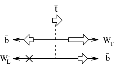
Figure 2: Typical configurations in the decay of $\bar{t}$ with definite spin orientation. Transverse $W^{-}$ ($W^{-}_{T}$) tend to be emitted in the direction of the $\bar{t}$ spin orientation, while longitudinal $W^{-}$ ($W^{-}_{L}$) are emitted in the opposite direction due to helicity conservation. For $m_{t}\simeq 175$ GeV, $\bar{t}$ decays mainly to $W^{-}_{L}$, hence $\bar{b}$ is emitted more in the $\bar{t}$ spin direction.

Now suppose $t$ and $\bar{t}$ have their spins in the $\hat{{\bf{n}}}_{\|}$ direction. Then $\bar{b}$ will be emitted dominantly in the $\hat{{\bf{n}}}_{\|}$ direction. One can see from Fig. 3(a) that in this case $t$ is always attracted to the forward direction due to the attractive force between $t$ and $\bar{b}$.

Figure 3: Attractive force between $t$ and $\bar{b}$ when the $t$ and $\bar{t}$ spins are oriented in the (a) $\hat{{\bf{n}}}_{\|}$ direction, and in the (b) $-\hat{{\bf{n}}}_{\|}$ direction. The momentum transfer $\delta{\bf{p}}_{b}=-\delta{\bf{p}}_{\bar{t}}$ due to the attraction is indicated by thick black arrows.

The direction of the attractive force will be opposite if $t$ and $\bar{t}$ have their spins in the $-\hat{{\bf{n}}}_{\|}$ direction (Fig. 3(b)). Thus, polarized top quarks will be pulled in a definite (forward or backward) direction, and we may expect that a forward-backward asymmetric distribution of the top quark $\sim\kappa\,C_{\|}^{0}(\chi)\cos\theta_{te}$ is generated by the final-state interaction.

Incidentally, a forward-backward asymmetric distribution of the top quarks is also generated by the interference between the $S$-wave and $P$-wave $t\bar{t}$ pair-production amplitudes [6]. It is formally a quantity of the same order as the final-state interaction near threshold, since it arises as an ${\cal O}(\beta)={\cal O}(\alpha_{s})$ correction to the leading spherically symmetric distribution. Interestingly, we find that each $\cos\theta_{te}$ distribution has quite a different physical explanation for its generation mechanism, although it is a common feature that both originate from the interplay between QCD and electroweak interactions.

3.c Top Quark Polarization Vector

The Coulomb attraction between $t$ and $\bar{b}$ also modifies the top-quark polarization vector [19]. As we have seen previously, in the $\bar{t}$ decay, $\bar{b}$ tends to be emitted in the direction of the parent $\bar{t}$’s spin direction (Fig. 2). We then find from Fig. 3 that if the $t$ and $\bar{t}$ spins are oriented in the $\hat{{\bf{n}}}_{\|}$ direction, $t$ will be attracted to the forward direction due to the attraction by $\bar{b}$, and oppositely attracted to the backward direction if the $t$ and $\bar{t}$ spins are in the $-\hat{{\bf{n}}}_{\|}$ direction. This means that in the forward region ($\cos\theta_{te}\simeq 1$) the number of $t$’s with spin in $\hat{{\bf{n}}}_{\|}$ direction increases whereas in the backward region the number of those with spin in the opposite direction increases. Or equivalently, the $\hat{{\bf{n}}}_{\|}$-component of the top-quark polarization vector increases in the forward region and decreases in the backward region. We may thus conjecture that the top-quark polarization vector is modified as $\delta\mbox{\boldmath$\cal P$}\sim\kappa\cos\theta_{te}\,\hat{{\bf{n}}}_{\|}$ due to the interaction between $t$ and $\bar{b}$.

3.d $l^{+}$ Energy-Angular Distribution

Finally let us examine the effect of the Coulomb attraction between $b$ and $\bar{t}$ on the $l^{+}$ energy-angular distribution in the semi-leptonic decay of $t$. The $b$-quark from $t$ decay will be attracted in the direction of $\bar{t}$ due to the Coulomb interaction between these two particles. We show schematically typical configurations of the particles in the top-quark semi-leptonic decay in Fig. 4.

Figure 4: Typical configurations of the particles in semi-leptonic decay of $t$ when the $b$-quark is emitted in the $\bar{t}$ direction. Due to the boost by $W^{+}$, the energy-angle correlation of $l^{+}$ will be either “$E_{l}$ is small and $l^{+}$ emitted in $-{\bf{p}}_{t}$ direction” or “$E_{l}$ is large and $l^{+}$ emitted in ${\bf{p}}_{t}$ direction”.

It can be seen that if the probability for $b$ being emitted in the $\bar{t}$ direction increases, correspondingly the probability for particular $l^{+}$ energy-angular configurations increases. These configurations are either “$E_{l}$ is small and $l^{+}$ emitted in $-{\bf{p}}_{t}$ direction” or “$E_{l}$ is large and $l^{+}$ emitted in ${\bf{p}}_{t}$ direction”.

4 $l^{+}$ Energy-Angular Distribution

We present the formulas for the charged lepton energy-angular distribution in the decay of a top quark that is produced via ${e^{+}e^{-}}\rightarrow{t\bar{t}}$ near threshold. In the following, $x_{l}=2E_{l}/m_{t}$ and $\Omega_{l}$, respectively, denote the normalized energy and the solid angle of the charged lepton as defined in the rest frame of the parent top quark. For simplicity we neglect the decay of $W^{-}$ in our calculations.

4.a Factorizable Part

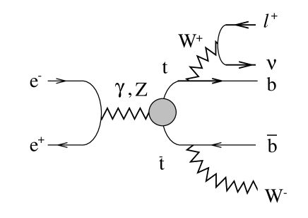
Figure 5: Born-type diagram for the process $e^{+}e^{-}\rightarrow t\bar{t}\rightarrow bl^{+}\nu\bar{b}W^{-}$.

It is well-known that the contribution of the Born-type (reducible) diagram (Fig. 5) to the differential distribution of $t$ and $l^{+}$ has a form where the production and decay processes of the top quark are factorized:

$$\frac{d\sigma_{\mbox{\scriptsize{Born}}}({e^{+}e^{-}}\!\rightarrow{t\bar{t}}\rightarrow bl^{+}\nu\bar{b}W^{-})}{d^{3}{\bf{p}}_{t}dx_{l}d\Omega_{l}}=\frac{d\sigma_{\mbox{\scriptsize{Born}}}(e^{+}e^{-}\!\rightarrow t\bar{t})}{d^{3}{\bf{p}}_{t}}\times\frac{1}{\Gamma_{t}}\,\frac{d\Gamma_{t\rightarrow bl^{+}\nu}(\mbox{\boldmath$\cal P$}_{\mbox{\scriptsize{Born}}})}{dx_{l}d\Omega_{l}}.$$ (4.1)

The above form holds true even including ${\cal O}(\alpha_{s})={\cal O}(\beta)$ corrections to each vertex and propagator in the Born-type diagram. Here, $\Gamma_{t}$ [22, 25] and $d\Gamma_{t\rightarrow bl^{+}\nu}(\mbox{\boldmath$\cal P$}_{\mbox{\scriptsize{Born}}})/dx_{l}d\Omega_{l}$ [24, 16], respectively, are the width of a free top quark and the charged lepton ($l^{+}$) energy-angular distribution in the decay of a free polarized top quark, both including the corresponding full ${\cal O}(\alpha_{s})~{}$corrections. Near threshold, the top-quark production cross section for longitudinally polarized $e^{+}e^{-}$ beams is given by [17, 19]

$$\frac{d\sigma_{\mbox{\scriptsize{Born}}}(e^{+}e^{-}\!\rightarrow t\bar{t})}{d^{3}{\bf p}_{t}}=\frac{d\sigma^{0}_{t\bar{t}}}{d^{3}{\bf p}_{t}}\times\left[1+2C_{FB}(\chi)\varphi_{\rm{}_{R}}(p,E)\cos\theta_{te}\right],$$ (4.2)

$$\frac{d\sigma^{0}_{t\bar{t}}}{d^{3}{\bf{p}}_{t}}=\frac{N_{c}\alpha^{2}\Gamma_{t}}{4\pi m_{t}^{4}}\,\left(1-P_{e^{+}}P_{e^{-}}\right)(a_{1}+\chi a_{2})\left(1-\frac{4C_{F}\alpha_{s}(m_{t})}{\pi}\right)\left|{\tilde{G}(p,E)}\right|^{2}.$$ (4.3)

Here, $\alpha$ is the fine structure constant, and $N_{c}=3$. $\mbox{\boldmath$\cal P$}_{\mbox{\scriptsize{Born}}}={\cal P}_{\|}\hat{{\bf{n}}}_{\|}+{\cal P}_{\bot}\hat{{\bf{n}}}_{\bot}+{\cal P}_{\rm N}\hat{{\bf{n}}}_{\rm N}$ represents the polarization vector of a top quark produced via the Born-type diagram (Fig. 5) near threshold. The components are given by

$${\cal P}_{\|}({\bf{p}}_{t},E,\chi) = C_{\|}^{0}(\chi)+C_{\|}^{1}(\chi)\,\varphi_{\rm{}_{R}}(p,E)\,\cos\theta_{te}\,$$ (4.4)

$${\cal P}_{\bot}({\bf{p}}_{t},E,\chi) = C_{\bot}(\chi)\,\varphi_{\rm{}_{R}}(p,E)\,\sin\theta_{te}\,$$ (4.5)

$${\cal P}_{\rm N}({\bf{p}}_{t},E,\chi) = C_{\rm N}(\chi)\varphi_{\rm{}_{I}}(p,E)\sin\theta_{te}\,.$$ (4.6)

Let us review briefly how to derive the factorized form of the differential distribution, Eq.(4.1). First, in calculating the fully-differential cross section $d\sigma/d\Phi_{5}(bl^{+}\nu\bar{b}W^{-})$, one may replace the top-quark momentum by an on-shell four-vector as

$$p_{t}^{\mu}=(p_{t}^{0},{\bf{p}}_{t})~{}~{}~{}\rightarrow~{}~{}~{}\tilde{p}_{t}^{\mu}=(\sqrt{{\bf{p}}_{t}^{2}+m_{t}^{2}},{\bf{p}}_{t})$$ (4.7)

in vertices and propagator numerators (but not in propagator denominators). The replacement is justified because near threshold relevant kinematical configurations are determined by

$$p_{t}^{0}-m_{t}\sim\alpha_{s}^{2}m_{t},~{}~{}~{}~{}~{}|{\bf{p}}_{t}|\sim\alpha_{s}m_{t}$$ (4.8)

so that the replacement induces differences only at ${\cal O}(\alpha_{s}^{2})$, and also because we will not be concerned with the $p_{t}^{0}$-dependence of the cross section. Then, one may use the following identity to factorize the spinor traces that appear in the fully-differential cross section into their production and decay parts: For an arbitrary $4\times 4$ spinor matrix $G$ and for a four-vector $\tilde{p}_{t}^{\mu}$ satisfying $\tilde{p}_{t}^{2}=m_{t}^{2}$,

$$\frac{\not\!\tilde{p}_{t}+m_{t}}{2m_{t}}\,G\,\frac{\not\!\tilde{p}_{t}+m_{t}}{2m_{t}}=\frac{\not\!\tilde{p}_{t}+m_{t}}{2m_{t}}\,\frac{1-\not\!{\cal P}\gamma_{5}}{2}\,C,$$ (4.9)

where the four-vector ${\cal P}^{\mu}$ and the constant $C$ are determined from $G$ and $\tilde{p}_{t}^{\mu}$ via the relation

$$\frac{1-{\cal P}\!\cdot\!s}{2}\,C=\mbox{Tr}\left[\frac{\not\!\tilde{p}_{t}+m_{t}}{2m_{t}}\,G\,\frac{\not\!\tilde{p}_{t}+m_{t}}{2m_{t}}\,\frac{1-\not\!s\gamma_{5}}{2}\right],$$ (4.10)

provided $s^{\mu}$ and ${\cal P}^{\mu}$ satisfy $s\cdot\tilde{p}_{t}={\cal P}\cdot\tilde{p}_{t}=0$.

One may also factorize the phase-space as

$$d\Phi_{5}(\gamma^{*}\rightarrow bl^{+}\nu\bar{b}W^{-})=\frac{d^{4}p_{t}}{(2\pi)^{4}}\,d\Phi_{3}(t^{*}\rightarrow bl^{+}\nu)\,d\Phi_{2}(\bar{t}^{*}\rightarrow\bar{b}W^{-}),$$ (4.11)

$$d\Phi_{3}(t^{*}\rightarrow bl^{+}\nu)=\biggl{(}\frac{1}{4\pi}\biggl{)}^{\!5}dx_{l}d\Omega_{l}dp_{W}^{2}d\phi_{bl},$$ (4.12)

where $p_{W}^{2}$ is the invariant-mass-squared of $l^{+}\nu$, and $\phi_{bl}$ denotes the azimuthal angle of $b$ around $l^{+}$ in the top-quark rest frame. Then one integrates over $dp_{W}^{2}$, $d\phi_{bl}$, $d\Phi_{2}(\bar{b}W^{-})$ and $dp_{t}^{0}/(2\pi)$; the integration over $p_{W}^{2}$ is trivial since we use the narrow-width approximation for $W^{+}$; the integration over $d\phi_{bl}$ is also trivial since the fully-differential cross section is independent of $\phi_{bl}$; the integration over the $\bar{b}W^{-}$ phase-space merely replaces the $\bar{b}W^{-}$ wave functions by $\Gamma_{t}$; the $p_{t}^{0}/(2\pi)$-integration is straightforward.

4.b Final-State Interaction Corrections

Corrections due to the final-state interactions (rescattering corrections) that originate from the irreducible diagrams (a)–(d) in Fig. 6 are important particularly in the threshold region.

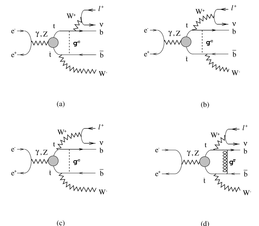
Figure 6: Diagrams for final-state interactions for $e^{+}e^{-}\rightarrow t\bar{t}\rightarrow bl^{+}\nu\bar{b}W^{-}$: (a) Coulomb-gluon exchange between $t$ and $\bar{b}$, (b) Coulomb-gluon exchange between $\bar{t}$ and ${b}$, (c) Coulomb-gluon exchange between $b$ and $\bar{b}$, and (d) transverse-gluon exchange between $b$ and $\bar{b}$.

In fact their contributions are counted as ${\cal O}(\alpha_{s})={\cal O}(\beta)$ corrections to the leading threshold enhancement [10]. We calculate the effect of each diagram on the $l^{+}$ energy-angular distribution. We chose Coulomb-gauge for the QCD part in our calculations.

The contribution of diagram (a) (exchange of one Coulomb-gluon between $t$ and $\bar{b}$) can be regarded, after integrating over the $\bar{b}W^{-}$ phase-space, as a correction to the production process of $t$. Thus, the production cross section $d\sigma_{\mbox{\scriptsize{Born}}}(e^{+}e^{-}\!\rightarrow t\bar{t})/d^{3}{\bf{p}}_{t}$ and the polarization vector $\mbox{\boldmath$\cal P$}_{\mbox{\scriptsize{Born}}}$ of the top quark receive corrections by this diagram, whereas the decay distribution $d\Gamma_{t\rightarrow bl^{+}\nu}(\mbox{\boldmath$\cal P$}_{\mbox{\scriptsize{Born}}})/dx_{l}d\Omega_{l}$ remains unaffected (except for the modification of $\mbox{\boldmath$\cal P$}_{\mbox{\scriptsize{Born}}}$). In fact the contribution of this diagram can be incorporated by the following substitutions in Eq. (4.1):

$$\frac{d\sigma_{\mbox{\scriptsize{Born}}}(e^{+}e^{-}\!\rightarrow t\bar{t})}{d^{3}{\bf p}_{t}}\rightarrow\frac{d\sigma_{\mbox{\scriptsize{Born}}}(e^{+}e^{-}\!\rightarrow t\bar{t})}{d^{3}{\bf p}_{t}}\times\left(1+\delta_{a}\right),~{}~{}~{}~{}~{}\mbox{\boldmath$\cal P$}_{\mbox{\scriptsize{Born}}}\rightarrow\mbox{\boldmath$\cal P$}_{\mbox{\scriptsize{Born}}}+\delta\mbox{\boldmath$\cal P$}_{a}$$ (4.13)

with

$$\delta_{a} = {\frac{1}{2}}\left[\psi_{1}(p,E)+\kappa C^{0}_{\|}\psi_{\rm{}_{R}}(p,E)\cos\theta_{te}\right],$$ (4.14)

$$\delta\mbox{\boldmath$\cal P$}_{a} = {\frac{1}{2}}\left[1-(C^{0}_{\|})^{2}\right]\kappa\,\psi_{\rm{}_{R}}(p,E)\cos\theta_{te}\cdot\hat{{\bf{n}}}_{\|}.$$ (4.15)

The derivation of the formula goes as follows. Since the relevant kinematical configuration lies in the soft gluon region, we can use soft-gluon approximation and factor out the part that depends on the loop-momentum $q^{\mu}$ (the propagators of the gluon, $\bar{b}$, $t$ and $\bar{t}$ together with the loop-integral) outside the spinor structure, while the remaining part is similar to the fully-differential cross section of the Born-type diagram. The latter part is factorized as before. Due to the soft-gluon factor (the factor pulled outside), at this stage we may interpret that the production cross section and polarization vector of top quark get corrections that depend on $t$ and $\bar{b}$ momenta. Integrations over $dp_{W}^{2}$ and $d\phi_{bl}$ are the same as for the Born-type diagram. For integrations over $d\Phi_{2}(\bar{b}W^{-})$, $dp_{t}^{0}/(2\pi)$ and $dq^{0}/(2\pi)$, we follow the method described in Ref.[10], Appendix D. We are thus led to Eqs. (4.13)–(4.15).

Diagram (b) (exchange of one Coulomb-gluon between $\bar{t}$ and $b$) in Fig. 6 gives a correction that connects the production and decay processes of the top quark. In fact one may incorporate the contribution of this diagram by multiplying Eq. (4.1) by a factor $[1+\xi(p,E,x_{l},\cos\theta_{lt})]$, where

$$\xi(p,E,x_{l},\cos\theta_{lt})=C_{F}\cdot 4\pi\alpha_{s}(\mu_{B})\int{\textstyle\frac{d^{3}{\bf{q}}}{(2\pi)^{3}}}\,\frac{1}{|{\bf{q}}\!-\!{\bf{p}}_{t}|^{3}}\,\mbox{Re}\left[\frac{\tilde{G}^{*}(q,E)}{\tilde{G}^{*}(p,E)}\,{\displaystyle\int^{2\pi}_{0}}\!{\textstyle\frac{d\phi_{bl}}{2\pi}}\,\frac{|{\bf{q}}\!-\!{\bf{p}}_{t}|}{\hat{{\bf{n}}}_{b}\!\cdot\!({\bf{q}}\!-\!{\bf{p}}_{t})+i\epsilon}\right].$$

(4.16)

$\hat{{\bf{n}}}_{b}$ denotes the unit vector in the direction of $b$. After integration over $d\Omega_{{\bf{q}}}d\phi_{bl}$, one may reduce the expression to a one-parameter integral form as

$$\xi(p,E,x_{l},\cos\theta_{lt})=C_{F}\cdot 4\pi\alpha_{s}(\mu_{B})\int^{\infty}_{0}\!dq\left\{w_{\rm{}_{R}}\,\mbox{Re}\biggl{[}\frac{\tilde{G}^{*}(q,E)}{\tilde{G}^{*}(p,E)}\biggl{]}\,+\,w_{\rm{}_{I}}\,\mbox{Im}\biggl{[}\frac{\tilde{G}^{*}(q,E)}{\tilde{G}^{*}(p,E)}\biggl{]}\right\}$$ (4.17)

with

$$w_{\rm{}_{R}}=\frac{1}{4\pi^{2}}\,\frac{q}{p^{2}-q^{2}}\left\{\theta(z_{+}^{2}\!-1)\cosh^{-1}|z_{+}|-\theta(z_{-}^{2}\!-1)\cosh^{-1}|z_{-}|\right\},$$ (4.18)

$$w_{\rm{}_{I}}=\frac{1}{4\pi^{2}}\,\frac{q}{|p^{2}-q^{2}|}\left\{\pi\theta\left((1+z_{+})(1+z_{-})\right)-\theta(1-z_{+}^{2})\cos^{-1}(z_{+})-\theta(1-z_{-}^{2})\cos^{-1}(z_{-})\right\},$$

(4.19)

$$z_{\pm}=\frac{q/p\pm\cos\theta_{Wl}\cos\theta_{lt}}{\sin\theta_{Wl}\sin\theta_{lt}},~{}~{}~{}\cos\theta_{Wl}=\frac{1+y}{1-y}-\frac{2y}{x_{l}(1-y)},~{}~{}~{}\cos\theta_{lt}=\frac{{\bf{p}}_{t}\cdot{\bf{p}}_{l}}{|{\bf{p}}_{t}||{\bf{p}}_{l}|}.$$ (4.20)

Here, $\theta_{Wl}$ represents the angle between $W^{+}$ and $l^{+}$ in the $t$ rest frame (given as a function of $x_{l}$); $\theta_{lt}$ represents the angle between $t$ and $l^{+}$ in the $t\bar{t}$ c.m. frame ($0\leq\theta_{Wl},\theta_{lt}\leq\pi$). The inverse functions $\cosh^{-1}$ and $\cos^{-1}$ in the above formulas take their values within $[0,\infty)$ and $[0,\pi]$, respectively. $\theta(x)$ is the unit step function. It is understood that the principal value should be taken in the integration of the $w_{\rm{}_{R}}$-term as $p\rightarrow q$.

We derived Eqs. (4.16) and (4.17) in the following manner. As in diagram (a), we used the soft-gluon approximation and factored out a soft-gluon factor (loop-integral of the propagators of gluon, $b$, $t$ and $\bar{t}$). The remaining part is same as the fully-differential cross section of the Born-type diagram except for the $t$ and $\bar{t}$ propagators and Green’s functions, which is again factorized. This time, however, the correction cannot be interpreted as associated with the top-quark production process since the soft-gluon factor depends on the $b$ momentum. The integrations over $dp_{W}^{2}$ and $d\Phi_{2}(\bar{b}W^{-})$ are the same as those for the Born-type diagram. The function $\xi$ given in Eq.(4.16) is essentially the soft-gluon factor integrated over $dp_{t}^{0}/(2\pi)$, $d^{4}q/(2\pi)^{4}$ and $d\phi_{bl}$. Finally, to derive Eq.(4.17) from (4.16), it is simpler to integrate over $d\Omega_{{\bf{q}}}$ before $d\phi_{bl}$.

Two noteworthy properties of $\xi(p,E,x_{l},\cos\theta_{lt})$ are: (1) its $l^{+}$-angular dependence enters only through $\cos\theta_{lt}$ and is independent of the angle from the $e^{-}$ beam direction or from the top-quark polarization vector, and (2) it is purely determined by the QCD interaction and free of the coupling parameters of electroweak interactions (except $y$).

As a non-trivial cross-check of the formula (4.17), we integrated $\xi\times\Gamma_{t}^{-1}d\Gamma_{t\rightarrow bl^{+}\nu}/dx_{l}d\Omega_{l}$ over the lepton energy-angular variables $\int dx_{l}d\Omega_{l}$ analytically and reproduced the one-parameter integral formula [10, 13] for the final-state interaction correction (from diagram (b)) to the top-quark three-momentum distribution.

The contribution of diagram (c) (exchange of one Coulomb-gluon between $b$ and $\bar{b}$) vanishes within our approximation. We show it in steps. Using soft-gluon approximation, the contribution of this diagram to the cross section can be written as

$$\frac{d\sigma_{c}}{d^{3}{\bf{p}}_{t}dx_{l}d\Omega_{l}} = \int{\textstyle\frac{dp^{0}_{t}}{(2\pi)}}\,dp_{W}^{2}\,d\phi_{bl}\,d\Phi_{2}(\bar{b}W^{-})\,\frac{1}{(2\pi)^{3}}\,\frac{1}{(4\pi)^{5}}\times T$$ (4.21)

$$\times iC_{F}\cdot 4\pi\alpha_{s}\int{\textstyle\frac{d^{4}k}{(2\pi)^{4}}}\,\left[D(p_{t})\!+\!D(p_{\bar{t}})\right]\left[D^{*}(p_{t}\!+\!k)\!+\!D^{*}(p_{\bar{t}}\!-\!k)\right]$$

$$~{}~{}~{}~{}~{}~{}~{}~{}~{}~{}~{}~{}~{}~{}~{}~{}\times\tilde{G}(p,E)\tilde{G}^{*}(|{\bf{p}}_{t}\!+\!{\bf{k}}|,E)\,\frac{1}{k^{0}-\hat{{\bf{n}}}_{b}\!\cdot\!{\bf{k}}-i\epsilon}\cdot\frac{1}{-k^{0}+\hat{{\bf{n}}}_{\bar{b}}\!\cdot\!{\bf{k}}-i\epsilon}\cdot\frac{1}{|{\bf{k}}|^{2}}$$

$$+\mbox{complex conj.},$$

where $k^{\mu}$ is the gluon momentum and

$$D(p_{t})=\frac{1}{p_{t}^{0}-m_{t}-{\bf{p}}_{t}^{2}/2m_{t}+i\Gamma_{t}/2}$$ (4.22)

denotes the non-relativistic top-quark propagator. $T$ is the contraction of hadronic and leptonic tensors resulting from the spinor traces after a soft-gluon factor (the second and third lines) is taken out. It coincides with the fully-differential cross section of the Born-type diagram except for the $t$ and $\bar{t}$ propagators and Green’s functions; hence $T$ is real. Next we integrate over $dp_{t}^{0}/(2\pi)$, $dk^{0}/(2\pi)$ and $d\Omega_{{\bf{k}}}$. Let us define

$$I({\bf{k}},\hat{{\bf{n}}}_{b},\hat{{\bf{n}}}_{\bar{b}})$$

$$\equiv~{}\int{\textstyle\frac{dp^{0}_{t}}{(2\pi)}\frac{dk^{0}}{(2\pi)}}\left[D(p_{t})\!+\!D(p_{\bar{t}})\right]\left[D^{*}(p_{t}\!+\!k)\!+\!D^{*}(p_{\bar{t}}\!-\!k)\right]\frac{1}{k^{0}-\hat{{\bf{n}}}_{b}\!\cdot\!{\bf{k}}-i\epsilon}\cdot\frac{1}{-k^{0}+\hat{{\bf{n}}}_{\bar{b}}\!\cdot\!{\bf{k}}-i\epsilon}$$

$$\simeq~{}\frac{1}{(\hat{{\bf{n}}}_{b}-\hat{{\bf{n}}}_{\bar{b}})\!\cdot\!{\bf{k}}+i\epsilon}\,\biggl{(}\frac{1}{\hat{{\bf{n}}}_{b}\!\cdot\!{\bf{k}}+i\Gamma_{t}}+\frac{1}{-\hat{{\bf{n}}}_{\bar{b}}\!\cdot\!{\bf{k}}+i\Gamma_{t}}\biggl{)}.$$ (4.23)

Noting that the contribution of diagram (c) to the cross section comes solely from the gluon momentum region

$$k^{0},|{\bf{k}}|\sim\alpha_{s}^{2}m_{t},$$ (4.24)

we keep $|{\bf{k}}|$ within this region. Then we may substitute $\tilde{G}^{*}(|{\bf{p}}_{t}+{\bf{k}}|,E)\rightarrow\tilde{G}^{*}(p,E)$ in Eq. (4.21) since the difference is higher order, and find

$$\frac{d\sigma_{c}}{d^{3}{\bf{p}}_{t}dx_{l}d\Omega_{l}} = \int dp_{W}^{2}\,d\phi_{bl}\,d\Phi_{2}(\bar{b}W^{-})\,\frac{1}{(2\pi)^{6}}\,\frac{1}{(4\pi)^{5}}\times T$$ (4.25)

$$\times iC_{F}\cdot 4\pi\alpha_{s}\left|{\tilde{G}(p,E)}\right|^{2}\times{\hbox to18.0pt{ \hbox to-3.0pt{$\displaystyle\int$} \raise-15.0pt\hbox to7.0pt{$\scriptstyle|{\bf{k}}|\sim\alpha_{s}^{2}m_{t}$} }}|{\bf{k}}|^{2}d|{\bf{k}}|\times\frac{1}{|{\bf{k}}|^{2}}\int d\Omega_{{\bf{k}}}\,I({\bf{k}},\hat{{\bf{n}}}_{b},\hat{{\bf{n}}}_{\bar{b}})$$

$$+$$ complex conj.

It is easy to see that $\int d\Omega_{{\bf{k}}}\,I({\bf{k}},\hat{{\bf{n}}}_{b},\hat{{\bf{n}}}_{\bar{b}})$ is real using the symmetry of $d\Omega_{{\bf{k}}}$ under ${\bf{k}}\rightarrow-{\bf{k}}$. Thus, we conclude $d\sigma_{c}/d^{3}{\bf{p}}_{t}dx_{l}d\Omega_{l}=0$ in our approximation.

In fact the same proof can be applied to show quite generally that the contribution of diagram (c) vanishes at ${\cal O}(\alpha_{s})~{}$provided one calculates a cross section where the top-quark energy is integrated out; for example, the top-quark three-momentum distribution. This is no longer the case when one considers a cross section that depends explicitly on the top-quark energy; for example, the top-quark four-momentum distribution. Then the diagram in question does contribute.

One can also show in a similar way that the kinematical regions Eq. (4.24) in diagrams (a) and (b) do not contribute to the cross section $d\sigma/d^{3}{\bf{p}}_{t}dx_{l}d\Omega_{l}$ and that only the gluon momentum region where $|{\bf{k}}|\sim\alpha_{s}m_{t}\gg\Gamma_{t}$ is relevant. We took advantage of this fact in deriving Eqs. (4.13)–(4.17).

It can be shown using similar techniques that the contribution of diagram (d) (exchange of one transverse gluon between $b$ and $\bar{b}$) gets canceled when it is added to that of the corresponding real-gluon emission diagram (interference of diagrams (e) and (f) in Fig. 7).

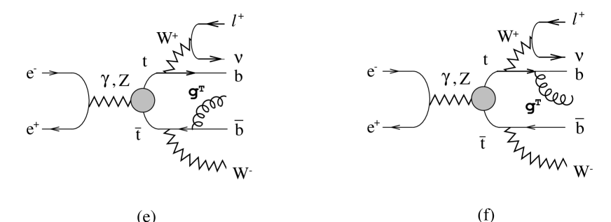
Figure 7: Diagrams for real-gluon emission process $e^{+}e^{-}\rightarrow t\bar{t}\rightarrow bl^{+}\nu\bar{b}W^{-}g$.

This cancellation is consistent with the same cancellation that was found in the calculation of the top-quark momentum distribution [10]. The contribution from each of these diagrams comes from the gluon momentum region $|{\bf{k}}|\hbox{ \raise 3.0pt\hbox to0.0pt{$<$}\raise-3.0pt\hbox{$\sim$} }\alpha_{s}^{2}m_{t}$ and is in fact logarithmically divergent due to a soft-gluon singularity.

The cancellations of the final-state interaction corrections at the various levels of inclusive cross sections are summarized in section 7.

Now let us compare our formulas and the argument given in the previous section. In subsections 3.b and 3.c, the parity-violating nature of the electroweak interactions in top production and decay played an essential role, while this was not the case in subsections 3.a and 3.d. We find that correspondingly the $\cos\theta_{te}$ term of $\delta_{a}$ and $\delta\mbox{\boldmath$\cal P$}_{a}$ contain electroweak coupling parameters (through $C^{0}_{\|}$), while the symmetric term of $\delta_{a}$ and $\xi$ are independent of these electroweak parameters. More precisely, the $\cos\theta_{te}$ term of $\delta_{a}$ and $\delta\mbox{\boldmath$\cal P$}_{a}$ have the forms anticipated in subsections 3.b and 3.c, respectively, if the function $\psi_{\rm{}_{R}}(p,E)$ is positive. Indeed, the numerical evaluation in Ref. [19] shows that $\psi_{\rm{}_{R}}(p,E)\hbox{ \raise 3.0pt\hbox to0.0pt{$>$}\raise-3.0pt\hbox{$\sim$} }0$ holds in the entire threshold region. Besides, an additional coefficient $\left[1-(C^{0}_{\|})^{2}\right]$ in $\delta\mbox{\boldmath$\cal P$}_{a}$ can be understood within our previous argument in the extreme cases $C^{0}_{\|}=\pm 1$. Namely, if the top quark is 100% polarized, there will be no contamination from the opposite spin so that the correction should disappear. It may be interesting to note that the final-state interaction corrections to the polarization vector vanishes for the ideally polarized top quarks, $C^{0}_{\|}=\pm 1$.

4.c Formula Including Full ${\cal O}(\alpha_{s})~{}$Corrections

In summary, the energy-angular distribution of $l^{+}$ including full ${\cal O}(\alpha_{s})={\cal O}(\beta)$ corrections can be cast into a form

$$\frac{d\sigma({e^{+}e^{-}}\!\rightarrow{t\bar{t}}\rightarrow bl^{+}\nu\bar{b}W^{-})}{d^{3}{\bf{p}}_{t}dx_{l}d\Omega_{l}}=\frac{d\sigma(e^{+}e^{-}\!\rightarrow t\bar{t})}{d^{3}{\bf{p}}_{t}}\times\frac{1}{\Gamma_{t}}\,\frac{d\Gamma_{t\rightarrow bl^{+}\nu}(\mbox{\boldmath$\cal P$})}{dx_{l}d\Omega_{l}}\times\left(1+\xi\right)$$ (4.26)

with

$$\frac{d\sigma(e^{+}e^{-}\!\rightarrow t\bar{t})}{d^{3}{\bf{p}}_{t}}=\frac{d\sigma^{0}_{t\bar{t}}}{d^{3}{\bf{p}}_{t}}\times\left[1+\frac{1}{2}\psi_{1}+(2C_{FB}\varphi_{\rm{}_{R}}+\frac{\kappa}{2}C_{\|}^{0}\psi_{\rm{}_{R}})\cos\theta_{te}\right],$$ (4.27)

$$\mbox{\boldmath$\cal P$}=\mbox{\boldmath$\cal P$}_{\mbox{\scriptsize{Born}}}+\delta\mbox{\boldmath$\cal P$}_{a}.$$ (4.28)

The above distribution is obtained as the sum of the cross sections for $e^{+}e^{-}\rightarrow t\bar{t}\rightarrow bl^{+}\nu\bar{b}W^{-}$ and $e^{+}e^{-}\rightarrow t\bar{t}\rightarrow bl^{+}\nu\bar{b}W^{-}g$. An independent emission of a gluon from the $t$ or $\bar{t}$ side has been included in Eq. (4.1), while the interference of both has been incorporated in conjunction with the final-state interaction diagram (d) in subsection 4.b.

Experimentally the top-quark four-momentum $p_{t}^{\mu}$ will necessarily be reconstructed from the $\bar{b}W^{-}$ system in the study of the $l^{+}$ distribution. For the case with a gluon in the final state, we assign the “top-quark momentum” as

$$\begin{array}[]{llll}\mbox{Case (A)}:&p_{t}\equiv(p_{e^{-}}+p_{e^{+}})-(p_{\bar{b}}+p_{W^{-}}+p_{g})&\mbox{if}&(p_{\bar{b}}+p_{W^{-}}+p_{g})^{2}-m_{t}^{2}\hbox{ \raise 3.0pt\hbox to0.0pt{$<$}\raise-3.0pt\hbox{$\sim$} }m_{t}\Gamma_{t},\\ \mbox{Case (B)}:&p_{t}\equiv(p_{e^{-}}+p_{e^{+}})-(p_{\bar{b}}+p_{W^{-}})&\mbox{if}&(p_{\bar{b}}+p_{W^{-}})^{2}-m_{t}^{2}\hbox{ \raise 3.0pt\hbox to0.0pt{$<$}\raise-3.0pt\hbox{$\sim$} }m_{t}\Gamma_{t}.\end{array}$$ (4.31)

(See, however, the discussion in section 7.) In other kinematical configurations the cross section is suppressed. Experimentally there will be a corresponding cut in the $\bar{b}W^{-}$ invariant mass. If both conditions in (A) and (B) are satisfied simultaneously, the gluon should necessarily be soft, and there will be no difference within our approximation between the cross sections corresponding to the above two assignments of the top-quark momentum.

One comment is in order here. In defining the “rest frame” of a top-quark in the study of $l^{+}$ distribution, one may use either $p_{t}^{\mu}$ or $\tilde{p}_{t}^{\mu}$ (defined in Eq.(4.7)). The difference of the cross sections based on the two definitions is of ${\cal O}(\alpha_{s}^{2})$ which is beyond the scope of our approximations. Thus, the cross sections defined in both definitions should be measured in experiment and compared. It will serve as a cross-check for the stability of our prediction.

5 Numerical Results

In this section we examine the effects of the final-state interaction corrections on the $l^{+}$ energy-angular distribution numerically, and compare the results with the qualitative argument given in section 3. The numerical results are obtained using both the coordinate-space approach developed in Refs. [2, 3] and the momentum-space approach developed in Refs. [4, 5]. Conventionally these two approaches have been used independently by different groups, and this is the first time to make a direct comparison of the cross sections calculated in both approaches. Some of the produced results are slightly different. We set $m_{t}=175$ GeV, $\alpha_{s}(M_{Z})=0.118$, $P_{e^{+}}=0$ and $\alpha=1/128$ in all our analyses.

We first examine the contribution of diagram (a) in Figs. 6 (Coulomb interaction between $t$ and $\bar{b}$) as given in Eqs. (4.13)–(4.15).

Figure 8: Top-quark momentum distributions $d\sigma/d|{\bf{p}}_{t}|$ obtained from Eq. (4.13) for various c.m. energies measured from the lowest-lying resonance, $\Delta E=\sqrt{s}-M_{1S}$. Solid lines and dashed lines represent the distributions with and without the final-state interaction between $t$ and $\bar{b}$ ($\delta_{a}$), respectively. We set $P_{e^{-}}=0$. The left figure corresponds to the coordinate-space calculation, the right one to the momentum-space calculation.

Shown in Fig. 8 are the top-quark momentum distribution $d\sigma/d|{\bf{p}}_{t}|$ for various c.m. energies measured from the lowest-lying resonance, $\Delta E=\sqrt{s}-M_{1S}$. This is calculated from the top-quark production cross section Eq. (4.13). As expected, the top-quark momentum is reduced. The effects are half in magnitude as compared to the final-state interaction corrections given in Refs. [10, 19] since only the interaction between $t$ and $\bar{b}$ is included here.

a) Coordinate-space approach results

b) Momentum-space approach results

Figure 9: Top-quark angular distribution $d\sigma/d\cos\theta_{te}$ obtained from Eq. (4.13) for various electron polarizations $P_{e^{-}}$. Solid lines and dashed lines represent the distributions with and without the final-state interaction between $t$ and $\bar{b}$ ($\delta_{a}$), respectively.

We show the angular distribution of the top-quarks in Figs. 9. It can be seen that the final-state interaction increases the top-quark distribution in the forward direction for $P_{e^{-}}=1$. This is consistent with our argument in subsection 3.b since in leading-order approximation $t$ and $\bar{t}$ have their spins aligned perfectly in the $\hat{{\bf{n}}}_{\|}$ direction for this $e^{-}$ polarization. Oppositely we see that the final-state interaction decreases the top-quark distribution in the forward direction for $P_{e^{-}}=-1$. We note that the top quark has a natural polarization $\mbox{\boldmath$\cal P$}\simeq-0.4\hat{{\bf{n}}}_{\|}$ for unpolarized $e^{+}e^{-}$ beams. Hence, the sign of the correction is the same as in the $P_{e^{-}}=-1$ case. Also we show corrections to the top-quark polarization vector in Fig. 10.

a) Coordinate-space approach results

b) Momentum-space approach results

Figure 10: Final-state interaction correction to the $\hat{{\bf{n}}}_{\|}$ component of the top-quark polarization vector, $\delta\mbox{\boldmath$\cal P$}_{a}$, for $P_{e^{-}}=+0.8$ (solid line), 0 (dash line), $-0.8$ (dot-dash line).

Although the qualitative behaviour meets our expectation, the magnitude of the correction is rather small. Note that $\delta\mbox{\boldmath$\cal P$}_{a}$ vanishes for $P_{e^{-}}=\pm 1$ since $C^{0}_{\|}=\pm 1$.

a) Coordinate-space approach results

b) Momentum-space approach results

Figure 11: Three-dimensional plots of $\xi$ as a function of $x_{l}$ ($x$-axis) and $\cos\theta_{te}$ ($y$-axis) at the peak momenta of the $|{\bf{p}}_{t}|$-distribution in Fig. 8: $\Delta E=0$ GeV and $\Delta E=5$ GeV.

Next we investigate the irreducible (non-factorizable) correction that stems from the Coulomb interaction between $\bar{t}$ and $b$. The correction factor $\xi(p,E,x_{l},\cos\theta_{lt})$ given in Eqs. (4.17)–(4.20) depends on four parameters, two of which specify the lepton configuration: $x_{l}$ and $\cos\theta_{lt}$. Therefore, we will examine the dependence of $\xi$ on these two parameters for several $(p,\Delta E)$ combinations. We fix the top-quark momentum $p$ to be the peak momentum of the distribution for each $\Delta E$, hence its values are slightly different for the two numerical approaches; see the top-quark momentum distributions in Fig. 8. Shown in Fig. 11 are 3-dimensional plots of $\xi$ as a function of $x_{l}$ and $\cos\theta_{lt}$. One can see that in the figures $\xi$ takes comparatively large positive values for either “small $x_{l}$ and $\cos\theta_{lt}\simeq-1$” or “large $x_{l}$ and $\cos\theta_{lt}\simeq+1$”. Oppositely, in the other two corners of the $x_{l}$–$\cos\theta_{lt}$ plane $\xi$ becomes small or becomes negative for smaller $\Delta E$. The typical magnitude of $\xi$ is 10–20%, which would be a reasonable size for an ${\cal O}(\alpha_{s})={\cal O}(\beta)$ correction. This behaviour holds also true for $\xi$ at $p$ off the peak of the top-quark momentum distribution. These features of the correction factor $\xi$ are consistent with our qualitative argument in section 3.

We made a cross-check of our numerical results for $\xi$ by numerically integrating $\xi\times\Gamma_{t}^{-1}d\Gamma_{t\rightarrow bl^{+}\nu}/dx_{l}d\Omega_{l}$ over the lepton energy-angular variables $\int dx_{l}d\Omega_{l}$ and comparing to the final-state interaction corrections to top-quark momentum distribution given in Refs. [10, 19].

It is seen that in Figs. 8 and 9 the coordinate-space approach and the momentum-space approach produce slightly different results. In particular the normalization of the cross sections differ at lower c.m. energies, $0\hbox{ \raise 3.0pt\hbox to0.0pt{$<$}\raise-3.0pt\hbox{$\sim$} }\Delta E\hbox{ \raise 3.0pt\hbox to0.0pt{$<$}\raise-3.0pt\hbox{$\sim$} }2$ GeV, whereas the differences decrease at higher energies. The cause of the differences can be traced back to the different short-distance QCD potentials employed in the two approaches. As we will discuss in section 7, this difference is formally counted as higher order beyond our approximation, and at present it should be taken as an uncertainty of the theoretical prediction.

6 Observable Proper to Top Decay Processes

As we have seen in the previous section, the final-state interactions affect the $l^{+}$ distribution in top-quark decays. The correction factor $\xi$ depends on the kinematical variables of both the top quark and $l^{+}$, and destroys the factorization of the cross section Eq. (4.1). In this section we define an observable which depends only on the top-quark decay process ($d\Gamma_{t\rightarrow bl^{+}\nu}/dx_{l}d\Omega_{l}$ of a free polarized top quark). It is a differential quantity dependent on the $l^{+}$ energy-angular variables.

From Eq. (4.17) one sees that the correction factor $\xi$ is invariant under the simultaneous transformations of the angular variables

$$\cos\theta_{Wl}\rightarrow-\cos\theta_{Wl},~{}~{}~{}~{}~{}\cos\theta_{lt}\rightarrow-\cos\theta_{lt},$$ (6.1)

since $z_{\pm}$ is invariant. This invariance may be understood as follows. The soft-gluon factor, which represents the final-state interaction in diagram (b) (Fig. 6), does not depend on the $l^{+}$ momentum as long as the $W^{+}$ momentum is kept fixed. One sees that accordingly the integrand of Eq. (4.16) is independent of the $l^{+}$ energy and angle. The dependence on these variables enters only through the phase-space integration over $\phi_{bl}$ for a given $l^{+}$ configuration. Therefore, one may reverse the $l^{+}$ momentum in the $t$ rest frame without affecting the phase-space integration, thereby keeping the whole function $\xi$ also unchanged. The above transformations Eq. (6.1) are essentially this reversal of the $l^{+}$ momentum. (Due to the form of the integrand, there are extra degrees of freedom for the transformation of the $l^{+}$ direction, see below.)

Using Eq. (4.20), the above transformation can be written as a transformation of the lepton energy and angle as

$$x_{l}\rightarrow x^{\prime}_{l}=\left(\frac{1+y}{y}-\frac{1}{x_{l}}\right)^{-1},~{}~{}~{}~{}~{}\hat{{\bf{n}}}_{l}\rightarrow\hat{{\bf{n}}}_{l}^{\prime}.$$ (6.2)

Here, $\hat{{\bf{n}}}_{l}={\bf{p}}_{l}/|{\bf{p}}_{l}|$ denotes the unit vector in the direction of $l^{+}$ in the top-quark rest frame. The choice of $\hat{{\bf{n}}}_{l}^{\prime}$ for flipping the sign of $\cos\theta_{lt}$ $(\cos\theta_{lt}\rightarrow-\cos\theta_{lt})$ is not unique. We represent by $\hat{{\bf{n}}}_{l}^{\prime}$ an arbitrary one of those choices. The production cross section of the top quark is not affected by this transformation since the top-quark kinematical variables are not involved. The important point is that neither the final-state interaction correction is affected by it.

Now, using this invariance, we first construct a quantity that has the simplest structure from the theoretical point of view, and afterwards we present an improved quantity that will be more useful for practical purposes. Let us define

$$A(x_{l},\hat{{\bf{n}}}_{l}\!\cdot\!\mbox{\boldmath$\cal P$},\hat{{\bf{n}}}_{l}^{\prime}\!\cdot\!\mbox{\boldmath$\cal P$})\equiv\left[\frac{d\sigma({e^{+}e^{-}}\!\rightarrow{t\bar{t}}\rightarrow bl^{+}\nu\bar{b}W^{-})}{d^{3}{\bf{p}}_{t}dx_{l}d\Omega_{l}}\right]\biggl{/}\left[\frac{d\sigma({e^{+}e^{-}}\!\rightarrow{t\bar{t}}\rightarrow bl^{+}\nu\bar{b}W^{-})}{d^{3}{\bf{p}}_{t}dx_{l}d\Omega_{l}}\right]_{\begin{array}[]{l}{\scriptstyle x_{l}\rightarrow x^{\prime}_{l}}\\ {\scriptstyle\hat{{\bf{n}}}_{l}\rightarrow\hat{{\bf{n}}}_{l}^{\prime}}\end{array}}.$$ (6.5)

(6.6)

The production cross section and the correction factor $\xi$ cancel in the numerator and denominator. As a result, this quantity is independent of the top-quark momentum ${\bf{p}}_{t}$ and is determined only from the free polarized top-quark decay cross section. In fact, using Eq. (4.26), we find that

$$A(x_{l},\hat{{\bf{n}}}_{l}\!\cdot\!\mbox{\boldmath$\cal P$},\hat{{\bf{n}}}_{l}^{\prime}\!\cdot\!\mbox{\boldmath$\cal P$})=\left[\frac{d\Gamma_{t\rightarrow bl^{+}\nu}(\mbox{\boldmath$\cal P$})}{dx_{l}d\Omega_{l}}\right]\biggl{/}\left[\frac{d\Gamma_{t\rightarrow bl^{+}\nu}(\mbox{\boldmath$\cal P$})}{dx_{l}d\Omega_{l}}\right]_{\begin{array}[]{l}{\scriptstyle x_{l}\rightarrow x^{\prime}_{l}}\\ {\scriptstyle\hat{{\bf{n}}}_{l}\rightarrow\hat{{\bf{n}}}_{l}^{\prime}}\end{array}}$$ (6.9)

holds up to (and including) ${\cal O}(\alpha_{s})={\cal O}(\beta)$ corrections. Note that the polarization vector $\cal P$, which specifies the decay distribution, includes the correction induced by the final-state interaction between $t$ and $\bar{b}$; see Eq. (4.28).

Since we take a ratio of differential cross sections in the definition of $A$ in Eq. (6.6), this quantity would suffer from a large statistical error experimentally. Meanwhile, this quantity is predicted to be dependent only on a few variables theoretically. (See Eq. (6.9).) It means that we may integrate out the irrelevant kinematical variables before taking the ratio and reduce its statistical uncertainty. For instance, we may choose $\hat{{\bf{n}}}_{l}^{\prime}=-\hat{{\bf{n}}}_{l}$ and define

$$\overline{A}(x_{l},a)\equiv\frac{\displaystyle\int{d^{3}{\bf{p}}_{t}d\Omega_{l}}\,\,\delta\!\left(\hat{{\bf{n}}}_{l}\!\cdot\!\mbox{\boldmath$\cal P$}-a\right)\left[\frac{d\sigma({e^{+}e^{-}}\!\rightarrow{t\bar{t}}\rightarrow bl^{+}\nu\bar{b}W^{-})}{d^{3}{\bf{p}}_{t}dx_{l}d\Omega_{l}}\right]~{}~{}~{}~{}~{}}{\displaystyle\int{d^{3}{\bf{p}}_{t}d\Omega_{l}}\,\,\delta\!\left(\hat{{\bf{n}}}_{l}\!\cdot\!\mbox{\boldmath$\cal P$}+a\right)\left[\frac{d\sigma({e^{+}e^{-}}\!\rightarrow{t\bar{t}}\rightarrow bl^{+}\nu\bar{b}W^{-})}{d^{3}{\bf{p}}_{t}dx_{l}d\Omega_{l}}\right]_{x_{l}\rightarrow x^{\prime}_{l}}}.$$ (6.10)

Here, the top-quark polarization vector in the delta functions should be evaluated as a function of ${\bf{p}}_{t}$ according to Eqs. (4.4)-(4.6), (4.15) and (4.28). The numerator and denominator, respectively, depend on two external kinematical variables and all other variables are integrated out.

Again using Eq. (4.26), one finds that $\overline{A}$ is determined solely from the free polarized top decays:

$$\overline{A}(x_{l},a)=\left[\frac{d\Gamma_{t\rightarrow bl^{+}\nu}(\mbox{\boldmath$\cal P$})}{dx_{l}d\Omega_{l}}\right]_{\scriptstyle\hat{{\bf{n}}}_{l}\!\cdot\!\mbox{\boldmath$\scriptstyle{\cal P}$}=a}\biggl{/}\left[\frac{d\Gamma_{t\rightarrow bl^{+}\nu}(\mbox{\boldmath$\cal P$})}{dx_{l}d\Omega_{l}}\right]_{\begin{array}[]{l}{\scriptstyle x_{l}\rightarrow x^{\prime}_{l}}\\ {\scriptstyle\hat{{\bf{n}}}_{l}\!\cdot\!\mbox{\boldmath$\scriptstyle{\cal P}$}=-a}\end{array}}.$$ (6.13)

This is a general formula that is valid even if the decay vertices of the top quark deviate from the standard-model forms. We see that the quantity $\overline{A}(x_{l},a)$ preserves most of the differential information contained in $d\Gamma_{t\rightarrow bl^{+}\nu}/dx_{l}d\Omega_{l}$.

7 Discussion

In this section we discuss three different issues relevant to our work. These are: the difference between the coordinate-space and momentum-space potentials, the mis-assignment of the top-quark momentum, and the disappearance of the final-state interaction corrections at the various levels of inclusive cross sections.

As we have seen in section 5, our numerical results obtained from the coordinate-space calculations and those obtained from the momentum-space calculations differ slightly, although all the qualitative features are common. The difference can be traced back to the difference in the short-distance part of the QCD potentials used in the two approaches.

Let us remind the reader how each potential is constructed (in the short-distance regime). The large-momentum part of the momentum-space potential $V_{\rm JKT}$ [4, 5] is determined as follows. First the potential has been calculated up to the next-to-leading order in a fixed-order calculation. The potential is then improved using the two-loop renormalization group equation in momentum space. On the other hand, the short-distance part of the coordinate-space potential $V_{\rm SFHMN}$ [3] is calculated by taking the Fourier transform of the fixed-order potential in momentum space, and then the potential is improved using the two-loop renormalization group equation in coordinate space. Thus, the two potentials are not the Fourier transforms of each other. Only the leading and next-to-leading logarithmic terms of the series expansion in a fixed $\overline{\rm MS}$-coupling are the same for the two potentials. The difference begins at the next-to-next-to-leading order terms. (The non-logarithmic term in the two-loop fixed-order correction.)

Figure 12: The effective charges (a) $\alpha_{\mbox{\scriptsize coor}}(1/r)$ and (b) $\alpha_{\mbox{\scriptsize mom}}(p)$ defined via the potentials in coordinate space and momentum space, respectively. $V_{\rm JKT}$ [4, 5] and $V_{\rm SFHMN}$ [3] represent the potentials used in the momentum-space approach and the coordinate-space approach, respectively.

To make a clear comparison, the two potentials are Fourier transformed numerically and we examine their difference both in coordinate space and in momentum space. We show the effective charges defined as

$$\alpha_{\mbox{\scriptsize coor}}(1/r)=\left(-C_{F}/r\right)^{-1}V(r),~{}~{}~{}~{}~{}\alpha_{\mbox{\scriptsize mom}}(q)=\left(-4\pi C_{F}/q^{2}\right)^{-1}\tilde{V}(q)$$ (7.1)

in Fig. 12, which clearly demonstrates that there is a non-negligible difference between the potentials. The oscillatory behaviour of $V_{\rm SFHMN}$ in Fig. 12(b) is an artifact due to the discontinuity in the second derivative of the coordinate-space potential, which is located at the continuation point of the perturbative potential to a long-distance potential. As already stated, the coordinate-space potential $V_{\rm SFHMN}$ follows the form required by the two-loop renormalization group equation in the short-distance region, whereas the momentum-space potential $V_{\rm JKT}$ follows the form required by the two-loop renormalization group equation in the large momentum region.

In principle we may reduce the difference by including the two-loop finite correction and invoking the three-loop renormalization group improvement [30]. We shall not do so in this paper, because there are a number of other corrections of the same order of magnitude which are not calculated yet. We will study the difference of the two approaches in more detail in a forthcoming paper.

In subsection 4.c, we assumed a perfect assignment of the top-quark momentum in cases (A) and (B) for defining the distribution formula, Eq. (4.26). In real experiments, however, a mis-assignment of the top-quark momentum will be inevitable whenever there is real gluon radiation in the final state because of the typical jet-clustering algorithm that will be used. For instance, when a gluon is indistinguishable from a $b$-jet, the top-quark momentum reconstructed by clustering may be off-shell; rather grouping the gluon on the other side (with $\bar{b}$) would result in an on-shell momentum. Ref. [10] studied how this mis-assignment alters the top-quark three-momentum distribution near threshold and found that the correction is less than a few percent; the clustering algorithm assumed in that paper, however, is somewhat unrealistic. The effect of the mis-assignment was also studied in Ref. [31] in the open-top region ($\sqrt{s}\gg 2m_{t}$) using a Monte Carlo generator and with more realistic experimental assumptions. It was shown that the effects on the top-quark invariant-mass distribution and on the angular distributions are substantial at $\sqrt{s}=400$ GeV (for $m_{t}=175$ GeV) and increase in magnitude and in complexity as the c.m. energy is raised. Clearly, in our case, we need more detailed studies to see how a similar effect may influence our results. For this purpose, studies based on a Monte Carlo generator that produces the fully-differential distribution including the full ${\cal O}(\alpha_{s})~{}$corrections near threshold would be necessary. (See also Ref. [12] for analyses on the radiative color flows from $t$, $\bar{t}$, $b$ and $\bar{b}$ close to the $t\bar{t}$ threshold.)

In the course of calculating the final-state interaction effects on the lepton energy-angular distribution, we found that the final-state interaction between $b$ and $\bar{b}$ vanishes (diagram (c) and (d)) if we add the corresponding real-emission diagram as well as if we integrate over the top-quark energy. This fact was already conjectured in Ref. [19] on account of an estimate of the Coulomb energy between $b$ and $\bar{b}$. Nevertheless the same final-state interaction modifies the top-quark energy distribution. As a similar phenomenon one may be reminded of the cancellation of final-state interactions (including also those between $t$ and $\bar{b}$) in the total $t\bar{t}$ production cross section, despite of the modification of the top-quark three-momentum distribution. In fact the cancellation of final-state interactions is a general feature known in a wide class of inclusive hard scattering cross sections both in QED and QCD.

Inclusiveness	Diagram (a)/(b)	Diagram (c)	Diagram (d)+(e)*(f)
fully differential	$+$	$+$	$+$
top energy integrated	$+$	vanish	vanish
$\sigma_{\rm tot}(s)$	vanish	vanish	vanish
typical gluon momentum	$\alpha_{s}m_{t}$	$\alpha_{s}^{2}m_{t}$	$\alpha_{s}^{2}m_{t}$

Table 1: Vanishment or non-vanishment of final-state interaction diagrams in the various inclusive cross sections. The plus sign “$+$” shows there is a non-canceled contribution from the diagram to the corresponding cross section, while “vanish” shows the cancellation of contributions from the diagram to the corresponding inclusive cross section. For details, see subsection 4.b.

It may be worth summarizing here at which level of inclusiveness the effects of the final-state interactions cancel in the various cross sections in our particular process, top quark pair production near threshold and its subsequent decay. This is shown in Table 1. Note that there are three typical mass scales involved in this process: the top-quark mass $m_{t}$, the inverse Bohr radius $\alpha_{s}m_{t}$, and the Coulomb energy between the $t\bar{t}$ pair $\alpha_{s}^{2}m_{t}$. We show in the table the typical momentum scale of the gluon in each diagram.

8 Conclusion

In this paper we considered the differential distribution of $l^{+}$ from the semi-leptonic decay of the top quark, where the parent top quark is produced in $e^{+}e^{-}\rightarrow t\bar{t}$ near threshold. Particularly, we have calculated the final-state interaction corrections (rescattering corrections) to the energy-angular distribution of leptons in the top quark decay. Also we have explicitly written down the $l^{+}$ energy-angular distribution ${d\sigma({e^{+}e^{-}}\!\rightarrow{t\bar{t}}\rightarrow bl^{+}\nu\bar{b}W^{-})}/{d^{3}{\bf{p}}_{t}dx_{l}d\Omega_{l}}$ including the full ${\cal O}(\alpha_{s})={\cal O}(\beta)$ corrections near threshold.

We presented numerical studies of the various effects of the final-state interaction corrections. All numerical results can be understood qualitatively from intuitive pictures. Attractive forces between $t$ and $\bar{b}$ and between $\bar{t}$ and $b$ modify not only the momentum distribution of $bW^{+}$ or $\bar{b}W^{-}$ system but also the top-quark polarization vector and the lepton energy-angular distribution.

• The effect of Coulomb-gluon exchange between $\bar{b}$ and $t$, when integrated over the $\bar{b}W^{-}$ phase-space, can be regarded as a correction to the top-quark production process. The effect can be incorporated by modifying the top-quark production cross section and the top-quark polarization vector. The top-quark momentum distribution is shifted to take a smaller average momentum due to the attraction by $\bar{b}$. Also since $\bar{b}$ is emitted preferably in the ${t}$ spin direction, the attraction generates a $\cos\theta_{te}$ distribution of the top quark as well as modifies the top-quark polarization vector.

• The Coulomb interaction between $b$ and $\bar{t}$ causes a non-factorizable correction with respect to the production and decay processes of the top quark. It generates an energy-angle-correlated correction to the lepton distribution. Namely, the $l^{+}$ distribution is deformed in favour of the kinematical configurations “small $E_{l}$ and emitted in $\bar{t}$ direction” or “large $E_{l}$ and emitted in $t$ direction”, which can be understood as originating from the attraction of $b$ in the direction of $\bar{t}$.

• Corrections from the gluon exchange between $b$ and $\bar{b}$ turn out to vanish when the top-quark energy is integrated out.

Without the non-factorizable effect $\xi$, the $l^{+}$ angular distribution is dependent only on the polar angle from the polarization vector of the parent top quark in its rest frame. The final-state interaction brings in another direction into the problem, the direction of $\bar{t}$, which is a completely new feature in comparison to the decays of free polarized top quarks.

In order to study the decay properties of top quarks near $t\bar{t}$ threshold, it is desirable to extract the part which is specific to the top-quark decay process alone. In the case of semi-leptonic decay, we defined a quantity which depends only on the decay distribution of a free polarized top quark. The part which depends on $\cos\theta_{te}$ and $\cos\theta_{lt}$ is dropped using the transformation of the $l^{+}$ energy and angle which leaves the final-state interaction unchanged. Thus, we recover a differential quantity $\overline{A}(x_{l},\hat{{\bf{n}}}_{l}\!\cdot\!\mbox{\boldmath$\cal P$})$ dependent only on the lepton energy and the lepton angle from the parent top-quark polarization vector.

This quantity will be useful from the theoretical point of view. It can be calculated from the decay distribution of free top quarks without including the bound-state effects or the final-state interaction corrections that are typical to the threshold region. Therefore, a variety of former studies on free top-quark decays may also be applicable in the $t\bar{t}$ threshold region, where highly polarized top quarks are available with the largest cross sections.

The authors wish to thank M. Jeżabek and J.H. Kühn for enlightening discussion.

References

- [1] V.S. Fadin and V.A. Khoze, JETP Lett. 46, 525 (1987); Sov. J. Nucl. Phys. 48, 309 (1988).
- [2] M. Strassler and M. Peskin, Phys. Rev. D43, 1500 (1991).
- [3] Y. Sumino, K. Fujii, K. Hagiwara, H. Murayama, and C.-K. Ng, Phys. Rev. D47, 56 (1993).
- [4] M. Jeżabek, J.H. Kühn and T. Teubner, Z. Phys. C 56 (1992) 653.
- [5] M. Jeżabek and T. Teubner, Z. Phys. C 59 (1993) 669.
- [6] H. Murayama and Y. Sumino, Phys. Rev. D47, 82 (1993).
- [7] P. Igo-Kemenes, M. Martinez, R. Miquel, and S. Orteu, Talk given at the Workshop on Physics and Experiments with Linear Colliders (Waikoloa, Hawaii, April 1993).
- [8] J.H. Kühn, in: F.A. Harris et al. (eds.), Physics and Experiments with Linear Colliders, Singapore: World Scientific, 1993, p.72.
- [9] K. Melnikov and O. Yakovlev, Phys. Lett. B324, 217 (1994).
- [10] Y. Sumino, PhD thesis, University of Tokyo 1993 (unpublished).
- [11] V. Fadin, V. Khoze, and A. Martin, Phys. Rev. D49, 2247 (1994); Phys. Lett. B320, 141 (1994).
- [12] V. Khoze and W. Sjöstrand, Phys. Lett. B328, 466 (1994).
- [13] K. Fujii, T. Matsui and Y. Sumino, Phys. Rev. D50, 4341 (1994).
- [14] W. Mödritsch and W. Kummer, Nucl. Phys. B430, 3 (1994); W. Kummer and W. Mödritsch, Z. Phys. C66, 225 (1995).
- [15] Y. Sumino, Acta Phys. Polonica B25 1837 (1994).
- [16] M. Jeżabek, in: T. Riemann and J. Blümlein (eds.), Physics at LEP200 and Beyond, Nucl. Phys. 37 B (Proc.Suppl.) (1994) 197.
- [17] R. Harlander, M. Jeżabek, J.H. Kühn and T. Teubner, Phys. Lett. B 346 (1995) 137.
- [18] W. Mödritsch, Nucl. Phys. B475, 507 (1996).
- [19] R. Harlander, M. Jeżabek, J. Kühn, and M. Peter, Z. Phys. C73, 477 (1997).
- [20] M. Jeżabek, Acta Phys. Polonica B 26 (1995) 789.
- [21] J.H. Kühn, Acta Phys. Polonica B 12 (1981) 347.
- [22] M. Jeżabek and J.H. Kühn, Nucl. Phys. B 314 (1989) 1.
- [23] M. Jeżabek and J.H. Kühn, Nucl. Phys. B 320 (1989) 20.
-
[24]
A. Czarnecki, M. Jeżabek and J.H. Kühn,
Nucl. Phys. B 351 (1991) 70;
A. Czarnecki and M. Jeżabek, Nucl. Phys. B 427 (1994) 3. - [25] M. Jeżabek and J.H. Kühn, Phys. Rev. D 48 (1993) R1910; erratum Phys. Rev. D 49 (1994) 4970
- [26] K. Melnikov and O. Yakovlev, Nucl. Phys. B471, 90 (1996).
- [27] V. Khoze and W. Stirling, Phys. Lett. B356, 373 (1995).
- [28] V. Khoze and W. Sjöstrand, Z. Phys. C70, 625 (1996).
- [29] W. Beenakker, A. Chapovsky and F. Berends, hep-ph/9706339 and hep-ph/9707326.
- [30] M. Peter, Phys. Rev. Lett. 78, 602 (1997) and hep-ph/9702245, Nucl. Phys. B in print.
- [31] C. Schmidt, Phys. Rev. D54, 3250 (1996).
- [32] V. Fadin, V. Khoze, A. Martin and A. Chapovskii, Phys. Rev. D52, 1377 (1995).