[

The Thermodynamics of Cosmic String densities in $U(1)$ Scalar Field Theory

Abstract

We present a full characterization of the phase transition in U(1) scalar field theory and of the associated vortex string thermodynamics in 3D. We show that phase transitions in the string densities exist and measure their critical exponents, both for the long string and the short loops. Evidence for a natural separation between these two string populations is presented. In particular our results strongly indicate that an infinite string population will only exist above the critical temperature. Canonical initial conditions for cosmic string evolution are show to correspond to the infinite temperature limit of the theory.

]

Topological defects appear in a great variety of systems from condensed matter laboratory experiments to the early Universe. Their importance in phase transitions in the laboratory is know to be fundamental and their presence in the early Universe may be the key to many of the unsolved questions in standard cosmology.

However, in spite of the universal relevance of topological defects, much about the fundamental description of their formation and evolution remains qualitative. This is a reflection of the complexities involved in first principle studies, owing to their nature as non-perturbative excitations of quantum field theories.

Particularly interesting for cosmology are string-like topological defects [1]. Motivated by the study of their creation in the early Universe [2], a variety of experiments has been recently developed with the aim of studying vortex string formation in liquid crystals [3], superfluid ⁴He [4] and ³He [5] systems. Their new results permit us to test with unprecedented precision theoretical ideas about defect formation and evolution.

From a theoretical standpoint, cosmic strings and other topological defects, have been traditionally thought to be produced at phase transitions in the early Universe as a result of the formation of correlated domains [6]. More recently a refinement of this scenario [7] has been gaining support, that most topological defects existing below the phase transition are, in fact, survivors of a population of unstable defects existing above the phase transition as non-linear excitations of the fields. In order to exist at low energies these field configurations need to be frozen in by some non-equilibrium process, which is context dependent. In a continuous phase transition, like the superfluid transition in ⁴He, this process may in addition be helped by the critical slowing down in the response of the fields close to the critical point. An estimate of the defect density hence produced is usually achieved given the correlation length of the field at the time of freeze out. By assigning random phases to different domains and connecting by the path of minimum phase gradient, a network of defects can in principle be constructed. This picture generates order of magnitude estimates that successfully predicted the defect densities observed in the Helium experiments.

In practice higher correlations in the phase structure of the fields exist and can change the picture considerably. As an illustration of the shortcomings of simply using the correlation length to predict produced defect densities note that similar densities would be estimated if the defect network were frozen in above or below the critical point, provided that the correlation length were chosen to be the same in both cases. This is clearly not what is observed experimentally [4], suggesting that the string network must be very different in two circumstances were the domain structure can be expected to coincide.

In order to match theory to future, more accurate measurements, as well as for the sake of theoretical understanding it is highly desirable to generate more detailed predictions for the string density formed at phase transitions. In cosmology and in the laboratory, equilibrium is the natural starting point. If we know the statistics of strings at any given temperature the reference to the domain structure in the fields becomes obsolete, while the role of non-equilibrium in freezing in the string network, at least in some scales, can be expected to hold as usual.

In this Letter we present the full characterization of the behavior of the string densities with temperature in the U(1) scalar field theory. In doing so we go beyond existing studies in the XY (see eg. [8]) model, which belongs to the same universality class, especially in determining the behavior of infinite strings, measuring critical exponents associated with string densities and confronting our findings with cosmological scenarios of defect formation.

We first determine the field thermodynamics and locate the critical point. In order to drive the system to equilibrium we evolved the fields stochastically according to

$$\left(\partial_{t}^{2}-\nabla^{2}\right)\phi_{i}-m^{2}\phi_{i}+\lambda\phi_{i}\left(\sum_{j}\phi_{j}^{2}\right)+\eta\dot{\phi_{i}}=\xi_{i},$$ (1)

where $\{i,j\}\in{1,2}$. The stochastic variable $\xi_{i}({\bf x},t)$ is taken to be Gaussian, characterized by

$$\langle \xi_{i}({\bf x},t)\rangle=0,$$ (2)

$$\langle \xi_{i}({\bf x},t)\xi_{j}({\bf x^{\prime}},t^{\prime})\rangle={2\eta\over{\beta}}\delta({\bf x-x^{\prime}})\delta(t-t^{\prime})\delta_{ij}.$$ (3)

These relations ensure that detailed balance applies in equilibrium, which will result for large times at temperature $1/\beta$. We evolved the system Eq. (1-3) using a staggered-leapfrog method, on a lattice of size $100^{3}$. We chose the lattice spacing to be $\delta l=0.5$. We verified that the correlation length was always resolved by at least 4 points in each linear dimension, apart from the cases when $\beta\ll 1$. Around the critical point all physical scales become much larger than the lattice spacing. Universal quantities can then be measured and shown explicitly to be independent of this ultraviolet cutoff. Away from the critical point, at high or low temperatures, universality is lost in general. There, the results loose some of their physical meaning but retain model properties, that are interesting from a theoretical point of view. This will be the case of the infinite temperature limit of the theory.

An equivalent equilibrium state could have been obtained using lattice Monte Carlo methods. Also, from the equilibrium point of view, the second order time derivative is redundant. However, this work is intended to be the precursor to non-equilibrium studies of the relativistic field theory, where is is more natural to use a Langevin method such as ours, and the field equations are naturally second order in time derivatives.

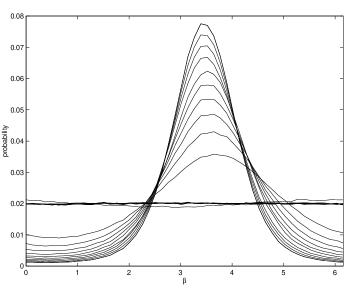
FIG. 1.: Phase probability distributions around the critical temperature for $\beta$ between 1.1 and 2.9 (steps of 0.1). For low temperatures the distribution becomes peaked around a randomly chosen phase. As the temperature increases the distribution becomes flat and the $U(1)$ symmetry is restored.

We decide when the system has reached equilibrium by monitoring several quantities associated with different length scales. We measure the kinetic energy of the system and check for equipartition. This characterizes the smallest scales in the sample. We monitor the string densities, associated with intermediate length scales and we measure the phase distribution functions across the whole volume. By making sure that these three quantities have reached asymptotic average values we conclude that the system is in equilibrium. The temperature of the bath coincides with that measured using equipartition.

The transition between a system displaying a prefered random direction in its manifold of field minima at low temperature and a flat phase distribution, characteristic of the $U(1)$ symmetry is shown in Fig. 1.

Although appealing the phase probability plots of Fig. 1 do not permit a precise determination of the critical temperature or any of its associated critical exponents. The critical point can be more easily found by observing the variation of the modulus of the spatial average of the field with the temperature:

$$\langle|\bar{\phi}|\rangle=\left\langle\sqrt{\sum_{i=1,2}\left({1\over{V}}\int_{V}d{\bf x}~{}\phi_{i}({\bf x})\right)^{2}}\right\rangle,$$ (4)

where the angular brackets denote ensemble averaging, obtained in practice by averaging over many independent measurements, $200-1000$, corresponding to well separated evolution times. The variation of Eq. (4) and its derivative with temperature is shown in Fig. 2. In particular we see that the derivative diverges at the critical point.

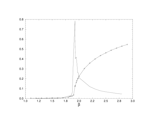
FIG. 2.: The variation of $\langle|\bar{\phi}|\rangle$ and its derivative, rescaled by $1/4$, with the temperature. Circles denote measured points. The divergence of the derivative marks the critical point.

The critical temperature can be measured by assuming that Eq. (4) behaves like

$$\langle|\bar{\phi}(\beta)|\rangle=A\;(\beta-\beta_{c})^{\alpha},$$ (5)

which is assumed to hold just below the critical temperature. By fitting our data at several temperatures to Eq. (5), for different choices of the inverse critical temperature $\beta_{c}$, we can determine its minimal $\chi^{2}$ value. Simultaneously we obtain the critical exponent $\alpha$. The critical values hence determined are $\beta_{c}=1.906\pm 0.008$ and $\alpha=0.43\pm 0.07$. The universal value of $\alpha$ is in reasonable agreement with renormalization group calculations [9].

Having measured the critical behavior in the fields we want to analyze how vortex string densities vary with the temperature. We assume ergodicity of the field evolution once equilibrium is reached. Using this fact we analyze at given time intervals the phase of the complex field, and associate a vortex to each 2-D lattice cell where the $U(1)$ phase winds through $2\pi$. We then proceed to connect the vortices and construct the string network. Given a string network, we measure the string density in loops and long string, for different values of the bath temperature around the phase transition.

Fig. 3 shows how the total density per lattice link of strings $\rho_{tot}$, as well as the density of long and short string ($\rho_{i}$ and $\rho_{l}$ respectively) changes with temperature. These quantities allow us a direct comparison to algorithms of cosmic string formation.

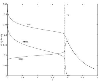
FIG. 3.: The lattice link densities of total string $\rho_{tot}$, loops $\rho_{l}$ and infinite string $\rho_{i}$ as a function of inverse temperature $\beta$ .

We observe a dramatic change in the behavior of the string system across the phase transition. The curves of fig. 3 suggest that we can decompose strings into two distinct populations, one of loops, say strings smaller than a certain cutoff length $L_{\infty}$ of the order of the squared linear dimension of our total volume and another population consisting of much longer strings. We will refer to the former as the string loop population and to the latter, owing to the usual terminology in cosmology, as infinite strings.

At $\beta_{c}$ all three densities display abrupt changes in their behavior. These changes are phase transitions as in all three cases the derivatives of the densities present discontinuities at the critical point. Even more remarkable is the fact that the appearance of infinite string seems to be linked to the criticality in the fields. The very sharp rise in the infinite string density at the critical point may suggest that the phase transition associated with it may actually be discontinuous in the infinite volume limit.

In order to clarify this question we measured the infinite string density variation with $\beta$ for various values of $L_{\infty}$. The results are shown in Fig. 4. The temperature at which infinite strings first appear clearly depends on the choice of $L_{\infty}$ , getting closer to $\beta_{c}$ as it increases. We also verified that for smaller lattice sizes infinite string first appeared at lower temperatures, eg. in a $20^{3}$ computational domain there was infinite string as soon as $\beta=2.3$. Both these variations supply evidence that as the volume is increased the temperature at which infinite strings first appear migrates towards the critical point implying a discontinuous phase transition in $\rho_{i}$. At present it is however impossible to perform such extrapolation with full confidence.

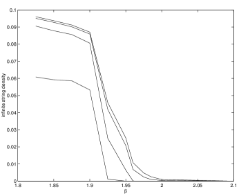
FIG. 4.: The dependence of $\rho_{i}$ on inverse Temperature, for $L_{\infty}=2500,8000,20000,100000$ (top to bottom), measured in lattice units.

We can establish that the phase transition in the fields and in the string densities coincide by finding the critical point and exponents for the latter.

At the critical temperature the density of strings drops suddenly and keeps falling for lower temperatures. The decay of $\rho_{tot}$ which coincides with $\rho_{l}$, is excellently described by the exponential law

$$\rho_{tot}(\beta)=\rho_{\rm tot}(\beta_{c})e^{-(\beta-\beta_{c})E}$$ (6)

where $\rho_{tot}(\beta_{c})\simeq 0.2$ is a universal number (see eg. [8] for a very different study yielding the same result) and $E=1.836$, implying that at temperatures below the critical point strings are Boltzmann suppressed. At low temperatures (in practice for $\beta\gtrsim 6$) there is long range order and no strings survive.

Just above the critical temperature the variation of the string densities can be best characterized by defining the quantity $\delta\rho\equiv(\rho(T)-\rho(T_{c}))/\rho(T_{c})$. The behavior of the infinite string density $\rho_{i}$ is well described by an ansatz similar to Eq. (5),

$$\delta\rho_{i}\propto(T-T_{c})^{\gamma_{i}}.$$ (7)

Note the change from $\beta$ in Eq. (5) to $T$ in Eq. (7). We find $\gamma_{i}=0.25\pm 0.01$ and $\beta_{c}=1.911\pm 0.001$, in agreement with all previous estimates. For $\rho_{tot}$ we find:

$$\delta\rho_{tot}\propto(T-T_{c})^{\gamma_{tot}},$$ (8)

with $\beta_{c}=1.912\pm 0.002$ and ${\gamma_{tot}}=0.39\pm 0.01$.

For temperatures well above the phase transition the loop density can be reasonably described by a quadratic form

$$\rho_{l}(\beta)\simeq\rho_{l}(0)\left(1+{\beta\over 3}-{1\over 3}({\beta\over 2})^{2}\right)$$ (9)

where $\rho_{l}(0)\simeq 1/12$. This corresponds to a fraction of $25\pm 1\%$ of all strings in loops for $\beta=0$.

The variations are much more complicated for $\rho_{tot}$ and $\rho_{i}$. The large size of the derivatives close to $\beta=0$ make it hard to approximate the curves and a successful fit can be achieved by a polynomial of very large degree, typically 9 or 10, with coefficients of alternating sign. Indeed, the behavior looks non-polynomial instead, which would mean that there is no standard high-temperature expansion for the infinite string density. This is explicable if we realize that there is no local operator which can distinguish an infinite string, and thus we would not necessarily expect a polynomial behavior around $\beta=0$.

Particularly interesting is the infinite temperature limit. We observe that then the total string density per link tends to $\rho_{tot}(0)=1/3$ and that its fraction of long strings tends to $75\pm 1\%$. These results coincide with those obtained from the canonical Vachaspati-Vilenkin (VV) algorithms for simulating string formation in the early Universe [10, 11, 12]. Their underlying motivation results from the picture that strings should result from random phase fluctuations within spatial domains of a given size. Typically, the complex field is given unit modulus, with phases assigned randomly to each site on a cubic lattice. There are variations on this theme: for example, the continuous phase may be approximated by three values [10], which leads to a slightly different string density and infinite string fraction. Nonetheless, assigning phases randomly to each lattice site corresponds precisely to the infinite temperature limit, and thus VV algorithms generate ensembles of string at infinite temperature. These ensembles are used as initial conditions for the free evolution of the string network, using a numerical solution to the classical dynamics of relativistic strings [1]. Thus numerical simulations of this type model an instantaneous quench from infinite to zero temperature. While these initial conditions are ultimately unphysical, the network of strings is observed to approach rapidly a self-similar evolution, which serves to disguise the initial state. On the other hand, if one would like to describe a network of strings below the critical point the Vachaspati-Vilenkin algorithm would be a completely inappropriate starting point.

Finally, our observation that the phase transition in the fields may coincide with the point when infinite string starts forming, suggests that strings do indeed play a fundamental role in the critical behavior of the system, as has been suggested so often in the literature [13, 14, 15, 16]. On the other hand, statistical studies of string networks [17] commonly identify the critical point in string densities with the Ginzburg temperature $T_{G}<T_{c}$. Above we presented evidence for the coincidence of the critical behavior in the fields and in the strings at $T_{c}$. In a future publication [18], a closer look at the properties of the string length distribution and a more detailed scale dependence study will help to clarify these problems.

We thank the Department of Computer Science at the Technical University of Berlin and the Fujitsu/Imperial College Centre for Parallel Computing for generous allocation of supercomputer time. We thank Andy Yates for usage of his string tracing routine. NDA thanks Ed Copeland for useful comments. LMAB is supported by the Deutsches Forschung Gemeinschaft. NDA is supported by JNICT - Programa Praxis XXI, under contract BD/2794/93-RM. MH is supported by PPARC (UK), under grants B/93/AF/1642, GR/L12899, and GR/K55967. This work is partially supported by the European Science Foundation.

REFERENCES

- [1] M. Hindmarsh and T.W.B. Kibble, Rep. Prog. Phys. 58 477 (1995); A. Vilenkin and E.P.S. Shellard, Cosmic Strings and Other Topological Defects (Cambridge Univ. Press, Cambridge, 1994).
- [2] W. H. Zurek, Nature 317 505 (1985), Acta Physica Polonica B 24 1301 (1993).
- [3] I. Chuang, R. Durrer, N. Turok and B. Yurke, Science 251, 1336 (1991); M.J. Bowick, L. Chander, E. A. Schiff and A. M. Srivastava, Science 263, 943 (1994) 943.
- [4] P. C. Hendy et al., Nature 368, 315 (1994); ibid in Formation and Interaction of Topological Defects, edited by A.-C. Davis and R. Brandenberger, Plenum (New York), 379 (1995).
- [5] C. Bauerle et al., Nature 382, 332 (1996); V.M.H. Ruutu et al., Nature 382, 334 (1996).
- [6] T.W.B. Kibble, J. Phys. A 9, 1387 (1976).
- [7] W. H. Zurek, Phys. Rep. 276 177 (1996).
- [8] G. Kohring, R. E. Shrock and P. Wills, Phys. Rev. Lett. 57, 1358 (1986).
- [9] Z. C. Le Guillou and J. Zinn-Justin, Phys. Rev. B 21, 3976 (1980).
- [10] T. Vachaspati and A. Vilenkin, Phys. Rev. D 30, 2036 (1984).
- [11] A. Yates and T.W.B. Kibble, Phys. Lett. B 364, 149 (1995).
- [12] A. Achucarro, J. Borrill and A. R. Liddle, hep-ph/9702368.
- [13] L. Onsager, Nuovo Cimento Suppl. 6, 249 (1949).
- [14] R. P. Feynman, in Progress in Low Temperature Physics, edited by C. J. Gorter (North-Holland, Amsterdam, 1955), Vol. 1, p.17.
- [15] V. Kotsubo and G. A. Williams, Phys. Rev. B 33, 6106 (1986).
- [16] H. Kleinert, Gauge Fields in Condensed Matter Physics (World Scientific, Singapore, 1989).
- [17] E. J. Copeland et al., Physica A 179, 507 (1991).
- [18] N. D. Antunes, L. M. A. Bettencourt and M. Hindmarsh, in preparation.