FTUV/97-53,IFIC/97-54

hep-ph/9708209

Abstract

In this work we analyze a new piece present in the $\Delta F=2$ effective Lagrangian in models with extra vector-like quarks. This piece, which was not taken into account previously, is required in order to preserve gauge invariance once the unitarity of the CKM matrix is lost. We illustrate the effects of this new piece in both, CP conserving and CP violating processes.

July 1997

1 Introduction

In the Standard Theory of the Electroweak Interactions(ST) there remain two main topics to be understood: the spontaneous breaking of the gauge symmetry (the Higgs sector) and the origin of the families (the flavour problem, including CP violation).The first problem will be studied with great detail once the hadron machines in the TeV region (LHC) start to operate. Nevertheless to get more insight in the flavour problem, it is not now mandatory to explore new energy regions. Instead, by reaching high luminosity in “low” energy machines such as tau-charm or beauty factories, one can perform tests of the ST in the flavour sector, not previously done, and consequently try to look for potential new physics.

There are several theoretically well-founded extensions of the Standard Theory, not excluded by experimental data, and giving rise to large deviations of the ST predictions in the flavour sector. In this paper we are interested in models with an extended quark sector. In particular, models with additional vector-like quarks have been extensively studied in the literature [1, 2]. The most salient feature of this kind of theories is the presence of $Z^{0}$-mediated flavour changing neutral currents(FCNC) at tree level. The origin of FCNC can be traced back to the failure of unitarity of the Cabbibo-Kobayashi-Maskawa(CKM) mixing matrix V. For simplicity, if we add to the ST just a vector-like singlet quark with charge $Q=-\frac{1}{3}$, the down quark mass eigenstates will be a mixture of the four down quarks present in the model and consequently V will be a 3 x 4 submatrix of a 4 x 4 unitary matrix. The columns of V are no more ortogonal, therefore the model has $Z^{0}$-mediated FCNC in the down sector.

The usual strategy to confront these kind of models with experiments has been to take as effective Lagrangian for $\Delta F=1,2$ FCNC processes, the ST Lagrangian (one loop) plus the new tree-level contribution. Of course, when the experimental data are analyzed with this new Lagrangian, significant deviations of ST values of the matrix elements $V_{ij}$ can be obtained, and this fact has been taken into account as is the case for $V_{td}$ in the analysis of $B_{d}^{0}-\overline{B_{d}^{0}}$ mixing. What never has been taken into account in the calculation of the effective Lagrangian, is the deviations from unitarity of the CKM-matrix, for example:

$$\sum_{i=1}^{3}V_{ib}^{*}V_{id}=U_{bd}\neq 0$$ (1)

if $U_{bd}$ is different from zero, the box diagram for $B_{d}^{0}-\overline{B_{d}^{0}}$ is not gauge invariant, implying the existence of new contributions, previously not considered. Even worse, the $Z^{0}$-penguin is divergent, so a reanalysis of $\Delta F=2$ boxes and $\Delta F=1$ electroweak penguins is mandatory in this class of theories. In fact is quite easy to understand that the new pieces in the $\Delta F=2$ can be linear in the new physics($U_{bd}$), contrary to the tree level contribution that is quadratic in $U_{bd}$. In the ST $V_{ub}V_{ud}^{*}$ is changed by minus the sum of the c and t quark couplings, giving rise to cancellations of gauge dependent pieces( at the same time that the ultraviolet behavior of the graph is improved). In these theories and following Eq.(1) there remains a gauge-dependent piece proportional to $U_{bd}$, coming from the box. Of course new pieces must be present to make gauge invariant this linear piece in $U_{bd}$, but in any case it is evident that in the limit of small $U_{bd}$, a linear term will dominate over the quadratic one . So we can expect that this new contributions will become important when both ST and new physics give rise to contributions of the same order.

The goal of this paper is to find the pieces linear in $U_{bd}$, present in the $\Delta F=2$ effective Lagrangian, in theories with extra vector-like singlet quarks. In section 2 we present a brief review of the model in order to fix the notation. Section 3 is devoted to present the calculation of the new pieces in the $\Delta F=2$ effective Lagrangian, also some comments about the $\Delta F=1$ pieces are included. In section 4 we illustrate the numerical effect of the presence of the new piece linear in $U_{qp}$ both for CP conserving and CP violating processes. And finally in section 5 we present our conclusions, where it is stressed the necessity of making a general numerical reanalysis of the predictions of these kind of models.

2 Models with vector-like quarks

For simplicity we will take the standard $SU(2)\otimes U(1)$ gauge theory with the addition of one $Q=-\frac{1}{3}$ down vector-like quark, singlet under $SU(2)$. Therefore the quark content of the model will be in the weak basis:

$$\begin{array}[]{cccc}q_{Li}^{0}\equiv\left(\begin{array}[]{c}u_{L}^{0}\\ d_{L}^{0}\end{array}\right)_{i}&u_{Ri}^{0}&d_{R\alpha}^{0}&d_{L4}^{0}\\ \\ (1/2,1/3)&(0,4/3)&(0,-2/3)&(0,-2/3)\end{array}$$ (2)

where i=1,2,3 and $\alpha$=1,2,3,4, and the weak isospin and hypercharges have been written explicitly. The Yukawa sector of the model with the standard Higgs-doublet $H$ is:

$${\cal L}_{Y}=\overline{q}_{Li}^{0}\Gamma_{i\alpha}d_{R\alpha}^{0}H+\overline{q}_{Li}^{0}\Delta_{ij}u_{Rj}^{0}\widetilde{H}+\overline{d}_{L4}^{0}\Sigma_{\alpha}d_{R\alpha}^{0}+h.c.$$ (3)

in general one can take $\Delta_{ij}$ real and diagonal in such a way that the up weak basis is the same than the up mass basis. For the down sector we have to diagonalize the mass matrix$\left(\begin{array}[]{c}\Gamma\\ \Sigma\end{array}\right)$, what can be done through

$$\begin{array}[]{ccc}d_{L}^{0}=Ad_{L}&;&A=\left(\begin{array}[]{c}V\\ B\end{array}\right)\end{array}$$ (4)

and an irrelevant rotation of $d_{R}^{0}$ .$A$ is a (4x4) unitary matrix and $V$ is a (3x4) submatrix that will play the role of the CKM-matrix. The weak gauge currents can be written as :

$${\cal L}_{W} = \frac{g}{\sqrt{2}}\overline{u}_{Li}V_{i\alpha}\gamma^{\mu}d_{L\alpha}W_{\mu}$$

$${\cal L}_{Z} = \frac{g}{2\cos\theta_{W}}[\overline{u}_{Li}\gamma^{\mu}u_{Li}-\overline{d}_{L\alpha}U_{\alpha\beta}\gamma^{\mu}d_{L\beta}$$ (5)

$$-2\sin^{2}\theta_{W}J_{em}^{\mu}]Z_{\mu}$$

Now, the charged currents mixing matrix $V$ is a (3x4) CKM-matrix and the neutral current Lagrangian is not flavour conserving in the left-handed down sector owing to the fact that $d_{L}$ is vector-like. In this case

$$U_{\alpha\beta}=V_{\alpha i}^{\dagger}V_{i\beta}=\delta_{\alpha\beta}-B_{\alpha}^{*}B_{\beta}$$ (6)

where unitarity of $A$ has been used. A similar result is obtained for the Higgs couplings,

$${\cal L}_{H}=-\frac{g}{2M_{W}}\left[\overline{u}_{Li}m_{i}^{u}u_{Ri}+\overline{d}_{L\alpha}U_{\alpha\beta}m_{\beta}^{d}d_{R\beta}\right]H+h.c.$$ (7)

and again the coupling to the down quark does not conserve flavour, $m_{i}^{u}$ and $m_{\beta}^{d}$ are the up and down quark masses respectively. In summary, the main differences with the ST are the existence of four down quarks, the CKM-matrix is a (3x4) and consequently there appears FCNC in the down sector, both in the gauge and the Higgs couplings. As far as the independent flavour parameters are concerned, we can say that the counting is six angles and three phases, like in a standard four-generations model. Consequently one can use a standard-like parametrization of the (4x4) A matrix [3] or other one that has been advocated in the literature [4].

3 $\Delta F=2$ Lagrangian

From Eq.(5) it is evident that the graphs of figure 1 will contribute, at tree level, to all the processes where the flavour of the down quark $\alpha$ changes in two units (and so does $\beta$ too,$\alpha\neq\beta$). These graphs give rise to an effective $\Delta F=2$ Lagrangian of the form

$${\cal L}_{eff}^{Z}=-\frac{G_{F}}{\sqrt{2}}\left(\overline{\beta}_{L}\gamma^{\mu}\alpha_{L}\right)\left(\overline{\beta}_{L}\gamma_{\mu}\alpha_{L}\right)U_{\beta\alpha}^{2}$$ (8)

This piece is the new physics contribution that usually has been added to the ST-term in order to confront this model to the experimental data. The so called ST-contribution (of course at one loop) comes from the diagrams in figure 2. If the calculation is performed in a general $R_{\xi}$-gauge (including the graphs with the unphysical Higgses) the contribution we get is of the form

$${\cal L}_{eff}^{box}=-\frac{G_{F}\alpha}{\sqrt{2}4\pi\sin^{2}\theta_{W}}\left(\overline{\beta}_{L}\gamma^{\mu}\alpha_{L}\right)\left(\overline{\beta}_{L}\gamma_{\mu}\alpha_{L}\right)F_{\alpha\beta}$$ (9)

where $F_{\alpha\beta}$ is given by

$$F_{\alpha\beta}=2\sum_{i,j=1}^{3}V_{i\beta}^{*}V_{i\alpha}V_{j\beta}^{*}V_{j\beta}F(i,j,\xi)$$ (10)

and $F(i,j,\xi)$ in the zero external momenta and masses limit is a function of the masses of the up-quarks of type $i$ and $j$, also a function of $M_{W}$ and dependent on the gauge parameter $\xi$ and consequently not gauge-invariant(!). Note that $V$ is not unitary in this model, therefore Eq.(10) is different from the ST-result. In fact if we make use of the definition of $U_{\alpha\beta}$ in Eq.(6), it is straightforward to get

$$F_{\alpha\beta} = 2\sum_{i,j=2}^{3}V_{i\beta}^{*}V_{i\alpha}V_{j\alpha}^{*}V_{j\beta}[F(i,j,\xi)-F(i,1,\xi)-F(1,j,\xi)$$ (11)

$$+F(1,1,\xi)]+2U_{\beta\alpha}\sum_{i=2}^{3}V_{i\beta}^{*}V_{i\alpha}\left[F(i,1,\xi)-F(1,1,\xi)\right]$$

$$+2U_{\beta\alpha}\sum_{j=2}^{3}V_{j\beta}^{*}V_{j\alpha}\left[F(1,j,\xi)-F(1,1,\xi)\right]$$

$$+2U_{\beta\alpha}^{2}F(1,1,\xi)$$

The first piece (the double summatory) is gauge invariant and is the only piece that has been included in this kind of models. It is the Inami-Lim ST-box contribution [5], except for the values of the CKM-matrix to be used. From the point of view of gauge invariance, it is quite legitimate to use only this piece from Eq.(11), but the important question that immediately arises from Eq.(11) is if the other pieces can be bigger than the first one or even bigger than the tree level result. Before answering these questions we must stress that the terms in Eq.(11) linear and quadratic in $U_{\beta\alpha}$ are not gauge-invariant, so if these pieces can be important we must look for a new set of diagrams to restore the gauge invariance of these contributions.

Coming back to the previous question it is quite clear that in the limit in which the forth down quark decouples, we recover the ST-model and consequently $U_{\beta\alpha}$($\beta\neq\alpha$) goes to zero, but not $V_{i\beta}^{*}V_{i\alpha}$ for $\alpha,\beta=1,2,3$.This means that the pieces quadratic with $U_{\beta\alpha}$ goes to zero more rapidly than the terms lineal in $U_{\beta\alpha}V_{i\beta}^{*}V_{i\alpha}$. Therefore, the pieces lineal in $U_{\beta\alpha}$ in Eq.(11) will dominate the tree level Lagrangian in Eq.(8) at least in the small $U_{\beta\alpha}$ regime. So, a priori, there is not reason (except probably the loop expansion) to consider the tree level $\Delta F=2$ Lagrangian in Eq.(8) to be the leading new physics contribution and not the linear pieces in $U_{\beta\alpha}$ appearing in Eq.(9). At the end it will be the experimental precision that will dictate which piece is more important, but from the point of view of a perturbative treatment, it looks evident that a piece linear in the new physics must be more important than a quadratic one, provided we have enough experimental precision.

As far as the $U_{\beta\alpha}^{2}$ piece in Eq.(11) is concerned, we must point out that its contribution to Eq.(9) is of the order $G_{F}\alpha U_{\beta\alpha}^{2}$ compared to the tree level that is of order $G_{F}U_{\beta\alpha}^{2}$. Of course having FCNC at tree level, at one loop level we get radiative corrections to the tree level coupling, and this new piece is an order $\alpha$ correction to Eq.(8). So we will neglect this piece, we are not interested in the full one loop renormalization of this model, but in the leading corrections to the ST-result in any regime of the parameters. Our next task is to find out the other one loop contributions of order $U_{\beta\alpha}V_{i\beta}^{*}V_{i\alpha}$ and such that when summed up to the second and third pieces in Eq.(11) we get a gauge-invariant result. These other diagrams must have a $Z$-flavour changing vertex and another vertex where the change of flavour is generated by two $W$-vertices, so the kind of graphs we are looking for are those depicted in figure 3. The blob with a $W$ in these graphs means to attach a $W$ in the blob in all possible ways to the fermion line, in order to construct a one loop diagram. So the $W$ will give us the $V_{i\beta}^{*}V_{i\alpha}$ term, the $Z$ in the other vertex will introduce $U_{\beta\alpha}$. Therefore any introduction of new physics in the blob will contribute to a subdominant piece and consequently the blob in figure 3 must be calculated like a ST-diagram. Note that if the $Z$ couples in the blob to an external line, we have to take $U_{\beta\gamma}=\delta_{\beta\gamma}$ ($\alpha=1,2,3$), otherwise we would get a $U_{\beta\alpha}U_{\beta\gamma}V_{i\gamma}^{*}V_{i\alpha}$ piece that is subleading. Similar, in the blob we have to consider $\sum_{i=1}^{3}V_{i\beta}^{*}V_{i\alpha}=\delta_{\beta\alpha}$, the remaining piece $B_{\beta}^{*}B_{\alpha}=U_{\beta\alpha}$ ($\alpha\neq\beta$) would give us $G_{F}\alpha U_{\beta\alpha}^{2}$ and therefore subleading again.

Now we have to show that the sum of the contribution of figure 3 and the two linear terms in $U_{\beta\alpha}$ of Eq.(11) gives a gauge-invariant result. First of all, the four diagrams in figure 3 give the same contribution, so we can concentrate in the first one. Second, both graphs in figure 2 gives the same contribution, so we can eliminate the global factor of 2 in Eq.(11) and concentrate in the first graph of this figure. In addition , the two terms linear in $U_{\beta\alpha}$ in Eq.(11) are equal because $F(i,j,\xi)$ is symmetric in $i,j$. Therefore we have to prove that the piece $U_{\beta\alpha}\sum_{i=2}^{3}V_{i\beta}^{*}V_{i\alpha}[F(i,1,\xi)-F(1,1,\xi)]$ and the first graph of figure 3 sum up to a gauge-invariant result.

But this has been proved long time ago, again in the Inami-Lim‘s paper [5], because the sum is exactly the same sum that has to be done to calculate the short-distance effective Lagrangian for $K\rightarrow\mu\overline{\mu}$. In fact the sum of this two graphs gives the same result as the coefficient of the operator $(\overline{\beta}_{L}\gamma_{\mu}\alpha_{L})(\overline{\mu}_{L}\gamma^{\mu}\mu_{L})$ but multiplied by $U_{\beta\alpha}$. Note that the piece we are talking about from the first graph in figure 2 correspond to perform the sum of $i$ using “unitarity” of $V$ and fixing $j=1$ ($m_{1}^{u}=0$ for the up-quark) and finally eliminating the two CKM-matrix from the $\beta j$ and $\alpha j$ vertices and multiply the global result by $U_{\beta\alpha}$. This box in the limit of zero external masses and momenta is the same box as the one we get for $\alpha\overline{\beta}\rightarrow\mu\overline{\mu}$ except for the global $U_{\beta\alpha}$ factor. The same happens for the $Z$-exchange graph, except that one must be careful in taking from the $\alpha\overline{\beta}\rightarrow\mu\overline{\mu}$ amplitude only the piece that is proportional to the weak isospin of the muon. Note that this piece is pure left-handed, while the piece proportional to the charge is pure vector and does not contribute to $K\rightarrow\mu\overline{\mu}$. Therefore we get for the total piece linear in $U_{\beta\alpha}$ four times the piece that Inami and Lim got for the coefficient of the operator $(\overline{s}_{L}\gamma^{\mu}d_{L})(\overline{\mu}_{L}\gamma^{\mu}\mu_{L})$, that of course is gauge-invariant. But this is in the quark amplitude, at the effective Lagrangian level we have to divide by 2x2.

Our full effective $\Delta F=2$ Lagrangian, neglecting external masses and momenta will be:

$${\cal L}_{eff}^{\Delta F=2} = \frac{G_{F}}{\sqrt{2}}\left(\overline{\beta}_{L}\gamma^{\mu}\alpha_{L}\right)\left(\overline{\beta}_{L}\gamma_{\mu}\alpha_{L}\right)\times$$ (12)

$$\times\left\{-U_{\beta\alpha}^{2}+\frac{\alpha}{4\pi\sin^{2}\theta_{W}}\left[4\widetilde{C}U_{\beta\alpha}+\widetilde{E}\right]\right\}$$

where $\widetilde{C}$ and $\widetilde{E}$ are defined in reference [5] as

$$\widetilde{E} = \sum_{i,j=2}^{3}V_{i\beta}^{*}V_{i\alpha}V_{j\beta}^{*}V_{j\alpha}\overline{E}(x_{i},x_{j})$$

$$\widetilde{C} = \sum_{i,j=2}^{3}V_{i\beta}^{*}V_{i\alpha}\overline{C}(x_{i},x_{1}=0)$$ (13)

and $x_{i}=\left(m_{i}^{u}/M_{W}\right)^{2}$ as usual. Taking into account the actual values of the quark masses, these functions can be approximated by the following results

$$\overline{E}(x_{c},x_{c}) \simeq -x_{c}$$

$$\overline{E}(x_{t},x_{t}) = \frac{-4x_{t}+11x_{t}^{2}-x_{t}^{3}}{4(1-x_{t})^{2}}+\frac{3x_{t}^{3}\ln x_{t}}{2(1-x_{t})^{3}}$$

$$\overline{E}(x_{c},x_{t}) = \overline{E}(x_{t},x_{c})\simeq-x_{c}\left[\ln\frac{x_{t}}{x_{c}}-\frac{3x_{t}}{4\left(1-x_{t}\right)}-\frac{3x_{t}^{2}\ln x_{t}}{4(1-x_{t})^{2}}\right]$$

$$\overline{C}(x_{c}) \simeq x_{c}$$

$$\overline{C}(x_{t}) = \frac{x_{t}}{4}\left[\frac{4-x_{t}}{1-x_{t}}+\frac{3x_{t}\ln x_{t}}{(1-x_{t})^{2}}\right]$$ (14)

Equation(12) is our main result. In particular it is the second piece, linear in $U_{\beta\alpha}$, that we claim that has previously neglected, and that a priori cannot be excluded in comparison to the first one. In particular, in the small $U_{\beta\alpha}$ limit ( the small new physics limit ), it is clear that this piece will be more important than the tree level result.

At this point it must be also clear that the $Z$-mediated $\Delta F=1$ effective Lagrangian that usually has been used is perfectly correct because in this case the new physics contribution is linear with $U_{\beta\alpha}$, and therefore any new physics introduced at one loop will be subleading. This is not the case for gamma mediated FCNC. They do not exist at tree level and consequently at one loop level one gets the ST-contribution and additional leading new physics [6]. This piece contributes for example to $b\rightarrow s\gamma$ and has been studied in [7].

4 Numerical analysis

In this section we will show the effects of our new contribution in Eq.(12). It must be stressed that it is in the $B_{d}$ system where there is a bigger window for the type of models we are considering. $B-\overline{B}$ mixing still can be dominated by the new contribution in the case of models with one extra down-type vector-like quark (dVLQ). But as it was pointed out in the previous section, the new contribution has more chances to become important in the case that the new physics is relatively small. It was shown in reference [2] that in CP asymmetries in $B$ decays [8] there can be big effects of physics beyond the standard one. The reason for that is that what is important in this case is the resulting phase in $B^{0}_{d}-\overline{B}^{0}_{d}$ mixing. With a 20% of new physics in the mixing of $B_{d}$, the authors of reference [2] showed spectacular effects for the CP asymmetry in the $J/\psi\,K_{S}$ and $\pi\pi$ channels, because the phase of the $U^{2}_{\beta\alpha}$ piece can be completly different to the standard model phase. Now looking at Eq.(12), we see that we are introducing a new piece $\tilde{C}U_{\beta\alpha}$ with a new phase. If the balance of magnitudes is fortunate (or unfortunate) enough, it could happen that we get an important enhancement of the new physics, but in any case it seems quite clear that previous results have to be revised. Therefore we will concentrate on the specific case of CP asymmetries in $B_{d}$ decays.

Following reference [2] and using Eq.(12) we get for the off diagonal term of the $B_{d}$ mixing matrix $M_{12}$

$$M_{12}=M_{12}^{(SM)}\Delta_{bd}^{*}$$ (15)

where $M_{12}^{(SM)}$ is the standard model contribution and $\Delta_{bd}$ is given by

$$\Delta_{bd}=1+are^{i\phi}-br^{2}e^{2i\phi}$$ (16)

where

$$re^{i\phi}=\frac{U_{bd}}{\lambda_{t}}\;,$$ (17)

$$\lambda_{t}=V_{tb}^{*}V_{td}\;,$$ (18)

$$a=\frac{4\overline{C}(x_{t})}{\overline{E}(x_{t})}\;,$$ (19)

and

$$b=\frac{4\pi\sin^{2}\theta_{W}}{\alpha}\frac{1}{\overline{E}(x_{t})}$$ (20)

for the actual top mass [9] we get

$$a=-3.271\;\;\mbox{and}\;\;b=-164.78$$ (21)

If we take into account that the actual bound for $r$ is $r\leq.3$ (see reference [10]), we conclude that the contribution of figure 1 (the piece with $b$, quadratic in $r$) can be at maximum 16 times bigger that the new piece (the piece with $a$, linear in $r$). But this is in the case where the new physics completely overwhelms the standard model contribution. In the interesting case studied by Branco et al. [2], where $-br^{2}=0.2$ ($r\simeq 0.035$) we get $ar=0.114$, therefore it is quite evident that the new piece is going to be important in this regime. Even more, if this 20% contributions give important effects, even in the case where the tree graph is important, and the new one loop piece is not too small we expect important deviations owing to the presence of a new phase.

In this model we have for the CP asymmetry in the $J/\psi\,K_{s}$ and $\pi\pi$ channels

$$a_{J} \equiv -\frac{\Gamma\left(B^{0}\longrightarrow J/\psi\,K_{s}\right)-\Gamma\left(\overline{B}^{0}\longrightarrow J/\psi\,K_{s}\right)}{\left(\sin(\Delta Mt)\right)\left(\Gamma\left(B^{0}\longrightarrow J/\psi\,K_{s}\right)+\Gamma\left(\overline{B}^{0}\longrightarrow J/\psi\,K_{s}\right)\right)}$$

$$= \sin\left(2\beta-\mbox{arg}(\Delta_{bd})\right)$$

$$a_{\pi} \equiv -\frac{\Gamma\left(B^{0}\longrightarrow\pi^{+}\pi^{-}\right)-\Gamma\left(\overline{B}^{0}\longrightarrow\pi^{+}\pi^{-}\right)}{\left(\sin(\Delta Mt)\right)\left(\Gamma\left(B^{0}\longrightarrow\pi^{+}\pi^{-}\right)+\Gamma\left(\overline{B}^{0}\longrightarrow\pi^{+}\pi^{-}\right)\right)}$$

$$= \sin\left(2\alpha+\mbox{arg}(\Delta_{bd})\right)$$

where $\alpha$ and $\beta$ are defined as usual

$$\alpha\equiv\mbox{arg}\left(-\frac{V_{td}V_{tb}^{*}}{V_{ud}V_{ub}^{*}}\right)$$ (24)

$$\beta\equiv\mbox{arg}\left(-\frac{V_{cd}V_{cb}^{*}}{V_{td}V_{tb}^{*}}\right)\;.$$ (25)

In order to plot $a_{J}$ and $a_{\pi}$ versus $\phi$ for a given value of $r$, to see how the new physics can change the standard model value and to clarify the effects of the new piece, let us explain over the unitarity quadrangle, the experimental input we need.

From figure 4, it is clear that with $r$ and $\phi$, the shape of the small upper traingle is fixed. We know experimentally two sides of the lower triangle $\mid V_{cd}V_{cb}^{*}\mid$ and $\mid V_{ud}V_{ub}^{*}\mid$, therefore to recontruct $\alpha$ and $\beta$ we need the third side of the lower triangle. But this can be accomplished by fixing the size of the small upper traingle through the experimental mixing parameter $x_{d}$

$$x_{d}=\frac{G_{F}\alpha_{\mbox{{\small em}}}}{6\pi\sqrt{2}\sin^{2}\theta_{W}}B_{B}f_{B}^{2}m_{B}\eta_{B}\tau_{B}\mid\lambda_{t}\mid^{2}\mid\overline{E}(x_{t},x_{t})\mid\mid\Delta_{bd}\mid$$ (26)

For a given value of $r$ and $\phi$, this formula fixes $\mid\lambda_{t}\mid$, so we know the full quadrangle (if possible), and therefore $\alpha$ and $\beta$.

In figures 5 and 6 we show the two asymmetries in a case similar to the one represented in reference [2]. In dashed lines we have plotted the actual prediction for the effective Lagrangian used previously to this work. In solid line, we present our new result. From the figures, it is quite evident that the deviation respect to the old results can be bigger than the expected sensitivities of B-factories, therefore we conclude that the new piece must be taken into account and therefore the whole Lagrangian in Eq.(12) must be used to look for vector-like contributions in CP asymmetries in $B$-decays. For completeness we also present,in figure 7, the CP conserving quantity $\mid\Delta_{bd}\mid$.

In figures 8 and 9 we represented a case where the new physics is more important (bigger $r$, $r=0.1$) and our new contribution should be less important from the moduli point of view. But in this case we get even more spectacular results, as previously announced because what is important in this case is the presence of new phases. In the figures there are regions where the unitarity quadrangle does not close and therefore there are forbidden regions in the $\phi$ space. Note that if we include the full Lagrangian (Eq.(12)) there is a region around $\phi=\pi$ that now is striclty forbidden. Near this region $a_{\pi}$ can change from -1 to 0 if we include our new piece.

5 Conclusions

In this work we have analyzed the effects of the previously omitted linear piece in $U_{bd}$ of the $\Delta F=2$ effective Lagrangian in theories with extra vector-like singlet quarks.

This term arises when one takes into account that due to the deviation of the CKM matrix from unitarity, the box diagram is not gauge invariant involving necessarily the presence of new contributions, not considered previously. This new piece, which is linear in $r$, has been shown to be important, not only in the small $r$ regime, but also in the big $r$ one. The reason was already given, it is because the new piece carries its own phase, which can be (and in general is) different from both the quadratic and standard model term phases.

Special emphasis was given to the consequences of this new piece for CP asymmetries in $B^{0}$ decays, which certainly can be quite important. In light of this, it seems clear that previous results have to be revised.

ACKNOWLEDGMENTS

It is a pleasure to thank O. Vives for his cooperation in part of this work and G. Branco for enlightening discussions. We would also like to thank J. Bernabéu and F. del Aguila for useful comments and discusions. G.B. acknowledges the Spanish Ministry of Foreign Affairs for a MUTIS fellowship . This work is supported by CICYT under grant AEN-96-1718 and IVEI under grant 038/96.

Figure 1: Tree level contributions to the $\Delta F=2$ Lagragian. These pieces are the new physics contribution that usually have been taken into account.

Figure 2: Standard Model contribution to the $\Delta F=2$ effective Lagrangian

Figure 3: New pieces which are linear in $U_{\beta\alpha}$

Figure 4: Unitarity quadrangle in the $B_{d}$ sector

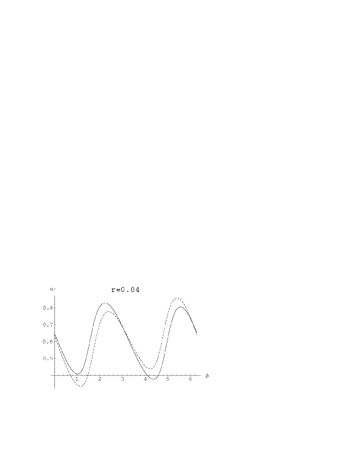
Figure 5: $a_{J}$ as a function of $\phi$ for $r=0.04$. The dashed line corresponds to the prediction obtained with the effective Lagrangian previously used (without the linear term), while the solid line corresponds to our new result.

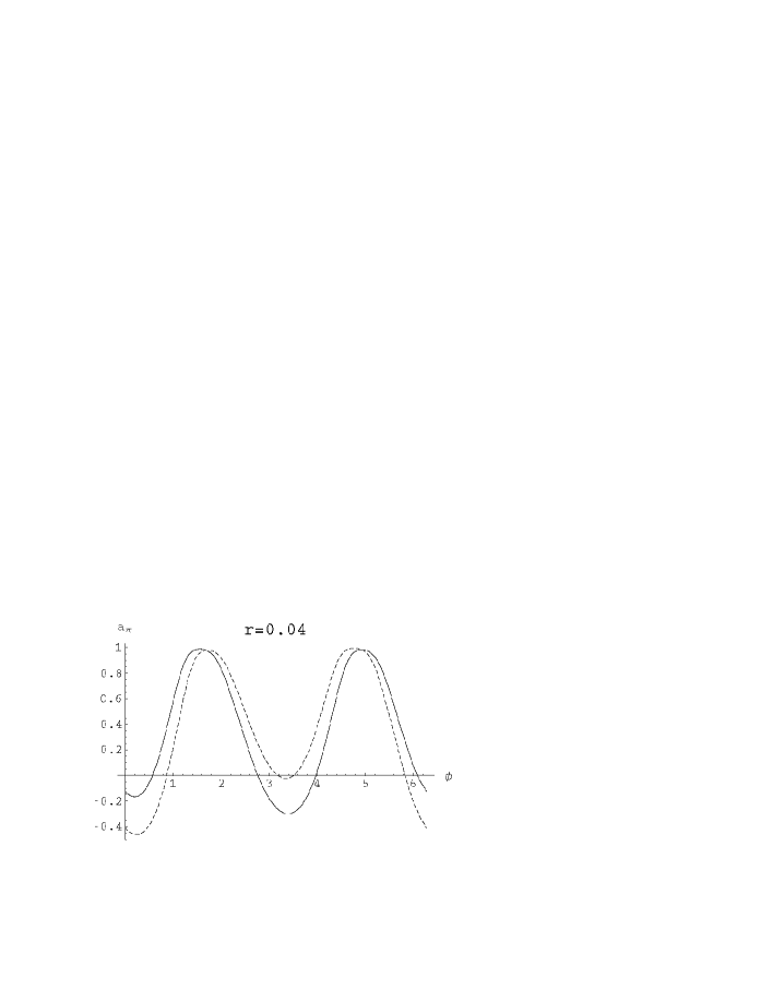
Figure 6: $a_{\pi}$ as a function of $\phi$ for $r=0.04$. The dashed line corresponds to the prediction obtained with the effective Lagrangian previously used (without the linear term), while the solid line corresponds to our new result.

Figure 7: $\mid\Delta_{bd}\mid$ as a function of $\phi$ for $r=0.04$. The dashed line corresponds to the prediction obtained with the effective Lagrangian previously used (without the linear term), while the solid line corresponds to our new result.

Figure 8: The same as figure 5 but with $r=0.1$. It is important to notice here that not all the values of $\phi$ are allowed.

Figure 9: The same as figure 6 but with $r=0.1$. Again some $\phi$ values are forbidden.

References

-
[1]
F.del Aguila and J.Cortés, Phys. Lett. B156 (1985) 243,
G.C.Branco and L.Lavoura, Nucl. Phys. B278 (1986) 738,
F.del Aguila, M.K.Chase and J.Cortés, Nucl. Phys. B271 (1986) 61,
Y.Nir and D.Silverman, Phys. Rev. D42 (1990) 1477,
D.Silverman, Phys. Rev. D45 (1992) 1800,
W-S.Choong and D.Silverman, Phys. Rev. D49 (1994) 2322,
V.Barger, M.S.Berger and R.J.N.Phillips, Phys. Rev. D52 (1995) 1663,
D.Silverman,Int. Jour. Mod. Phys. A11 (1996) 2253,
M.Gronau and D.London, Phys. Rev. D55 (1997) 2845,
F.del Aguila, J.A.Aguilar-Saavedra and G.C.Branco, UG-FT 69/97, hep.ph/9703410, March 1997. - [2] G.C.Branco, T.Morozumi, P.A.Parada and M.N.Rebelo, Phys. Rev. D48 (1993), 1167.
- [3] F.J.Botella and L.L.Chau, Phys. Lett. 168B (1986) 97.
- [4] V.Barger, K.Whisnant and R.J.N.Phillips, \pdD23 (1981) 2773.
- [5] C.S. Lim and T. Inami, Prog. Theor. Phys. 65 (1981) 297.
- [6] J.Roldán, F.J.Botella and J.Vidal, Phys. Lett. B283 (1992) 389.
- [7] L.T.Handoko and T.Morozumi, Mod. Phys. Lett. A10 (1995) 309.
- [8] For the general formalism of CP asymmetries in neutral decays, see e.g, Y.Nir and H.Quinn, Ann. Rev. Nucl. Part. Sci. 42 (1992) 211.
- [9] A.J.Buras and R.Fleischer, Quark mixing, CP violation and rare decays after the top quark discovery , to appear in Heavy Flavour II, eds. A.J.Buras and M.Lindner, Advanced Series on Directions in High Energy Physics, World Scientific (1997).
- [10] Y.Grossman, Y.Nir and R.Rattazzi, CP violation beyond the Standard Model, to appear in Heavy Flavour II, eds. A.J.Buras and M.Lindner, Advanced Series on Directions in High Energy Physics, World Scientific (1997).