Abstract

We investigate properties of the color space of $SU(N_{c})$ gauge theories in the limit of small number of colors ($N_{c}\to 0$) and large number of flavors. More generally, we introduce a rescaling of $\alpha_{s}$ and $n_{f}$ which assigns a finite limit to colored quantities as $N_{c}\to 0$, which reproduces their known large-$N_{c}$ limit, and which expresses them as an analytic function of $N_{c}^{2}$ for arbitrary value of $N_{c}$. The vanishing-$N_{c}$ limit has an Abelian character and is also the small-$N_{c}$ limit of $[U(1)]^{N_{c}-1}$. This limit does not have an obvious quantum field theory interpretation; however, it provides practical consistency checks on QCD perturbative quantities by comparing them to their QED counterparts. Our analysis also describes the two-dimensional topological structure involved in the interpretation of the small $N_{c}$-limit in color space.

Introduction

’t Hooft has shown the utility of studying gauge theories with internal symmetries in the limit of large number of colors [1]. In this note, we explore the analytic properties of formulae for non-Abelian theories taking the number of colors $N_{c}$ to zero and the number of flavors $n_{f}$ to infinity. Our underlying motivation is to attempt to uncover patterns in the group structure of $SU(N_{c})$ which encompasses a nontrivial set of values of $N_{c}$. Little is known about nontrivial values of $N_{c}$ except in the large $N_{c}$-limit, where it has been shown to have an interpretation in terms of a theory of membranes [2]. The value $N_{c}=0$ is another limit where we can expect simplifications to take place, hence, to provide additional clues as to what the theory is at finite $N_{c}$. The limit $N_{c}\to 0$ has already found some applications in condensed matter systems, in the context of spin glass [4] and localization phenomena [5]. Negative values of $N_{c}$ have been studied in a group-theoretic framework [6]. Furthermore, numerical work has shown that QCD₁₊₁ has a well-defined particle spectrum in the limit $N_{c},\,n_{f}/N_{c}\to\infty$ [7], a particular limit first introduced by Veneziano in QCD₄ [8]. The present analysis is to our knowledge, the first attempt to implement the limit $N_{c}\to 0$ in the context of gauge theories. In this investigation, we are not concerned with the meaning of the corresponding spacetime quantum theory but rather with the structure of the space of color degrees of freedom. Our analysis is preliminary, yet we find it suggestive of the existence of a deeper mathematical structure which covers a larger set of values of $N_{c}$. Specifically, the vanishing-$N_{c}$ limit singles out a point-like structure reflecting a cluster of interlinked punctures on a surface, in contrast with the two-dimensional objects characteristic of the large-$N_{c}$ limit.

To give meaning to a physical quantity as $N_{c}$ becomes vanishingly small, we need to provide a proper rescaling to the parameters of the theory. Clearly, we need the gauge coupling ${\widehat{\alpha}_{s}}\sim\alpha_{s}/N_{c}$, in order to compensate for the decrease the number of degree of freedom in the theory. When fermions are included, we also need to compensate accordingly, ${\widehat{n_{f}}}\sim n_{f}N_{c}$. These choices are natural since, as we soon show, they provide a finite value to all physical quantities and constitute the counterparts of those choices made in the large-$N_{c}$ limit: ${\widehat{\alpha}_{s}}\sim\alpha_{s}N_{c},{\widehat{n_{f}}}\sim n_{f}/N_{c}$ which, in this case, compensate for the ever-increasing number of fermionic and bosonic degrees of freedom [1, 8]. As we argue soon, it is constructive to conjecture that these rescalings are special cases of a unique, yet unknown, analytic rescaling in $N_{c}$. Such a universal rescaling would plausibly be of the form ${\widehat{\alpha}_{s}}\sim\alpha_{s}\,f(N_{c})/N_{c},{\widehat{n_{f}}}\sim n_{f}\,N_{c}/g(N_{c})$ with the functions $f(N_{c})$ and $g(N_{c})\sim N_{c}^{2}$ as $N_{c}$ becomes arbitrarily large and $f(0)\sim g(0)\sim\,const.$, in order to satisfy the above requirements.

Examples

We illustrate the above setting with a few examples of the behavior of QCD perturbative physical quantities under the tentative rescaling

$${\widehat{\alpha}_{s}}=\alpha_{s}\times\,{{\bf\Lambda}\over 2N_{c}}\hskip 56.9055pt{\widehat{n_{f}}}=n_{f}\times\,{N_{c}\over{\bf\Lambda}}.$$ (1)

where ${\bf\Lambda}$ is an unknown function of $N_{c}$ satisfying (${c_{\infty}}$, ${c_{0}}$ are nonzero integers)

$${\bf\Lambda}\rightarrow{c_{\infty}}\,N_{c}^{2}\ \ {\rm as}\ \ N_{c}\to\infty\hskip 42.67912pt{\rm and}\hskip 42.67912pt{\bf\Lambda}\rightarrow-{c_{0}}\ \ {\rm as}\ \ N_{c}\to 0\,.$$ (2)

It is worth noting that ${\bf\Lambda}$ can be chosen to be a linear function of $N_{c}^{2}$, $\,={c_{\infty}}N_{c}^{2}-{c_{0}}$. More generally, in what follows we assume that ${\bf\Lambda}$ is an analytic function of $N_{c}^{2}$. This assumption is not dictated by any fundamental principles but rather, is appealing for the simplicity of its consequences.

As a first example, let us look at the non-Abelian running coupling constant. It satisfies

$${1\over\alpha_{s}}\,{d\alpha_{s}\over d\ln Q^{2}}=-\beta_{0}{\alpha_{s}\over\pi}-\beta_{1}{\alpha_{s}^{2}\over\pi^{2}}+\cdots$$ (3)

with ($T=1/2$, ${C_{F}}=(N_{c}^{2}-1)/2N_{c}$)

$$\beta_{0}={11\over 12}N_{c}\,-\,{1\over 3}Tn_{f}\,,\hskip 56.9055pt\beta_{1}={17\over 24}N_{c}^{2}\,-\,\left({5\over 12}N_{c}+{{C_{F}}\over 4}\right)\,Tn_{f}\,.$$ (4)

Under the rescaling (1), these equations become

$${1\over{\widehat{\alpha}_{s}}}\,{d\widehat{\alpha}_{s}\over d\ln Q^{2}}=-\widehat{\beta}_{0}{\widehat{\alpha}_{s}\over\pi}-\widehat{\beta}_{1}{\widehat{\alpha}_{s}^{2}\over\pi^{2}}+\cdots\qquad{\rm with}\qquad\widehat{\beta}_{n}={\beta_{n}\times\,\left({2N_{c}\over{\bf\Lambda}}\right)^{n+1}}.$$ (5)

Explicit values for $\widehat{\beta}_{0}$ and $\widehat{\beta}_{1}$ are

$$\widehat{\beta}_{0}={11\over 12}{\widehat{N_{c}}}-{{\widehat{n_{f}}}\over 3}\,,\hskip 56.9055pt{\widehat{\beta}}_{1}={17\over 24}{\widehat{N_{c}}}^{2}-\left({5\over 12}{\widehat{N_{c}}}+{\widehat{C_{F}}\over 4}\right){\widehat{n_{f}}}$$ (6)

where for conciseness, we have introduced ${\widehat{N_{c}}}=N_{c}\times 2N_{c}/{\bf\Lambda}$ and $\widehat{C_{F}}={C_{F}}\times 2N_{c}/{\bf\Lambda}$ which have values $0$, $1/{c_{0}}$ at $N_{c}=0$ and values $2/{c_{\infty}}$, $1/{c_{\infty}}$ at $N_{c}=\infty$ respectively.

The expressions (5) and (6) are analytic functions of $N_{c}^{2}$ and are finite for all values of $N_{c}$ except possibly at zeroes of ${\bf\Lambda}$. A worth-noting peculiarity of these expressions is the change of sign of ${\widehat{\beta}}_{0}$ for sufficiently small values of $N_{c}$, conferring to the rescaled quantities an Abelian-like character in the vanishing-$N_{c}$ limit. These features are not accidental as we establish later.

In the particular limit $N_{c}\to 0$, ${\widehat{\beta}}_{0}$ and ${\widehat{\beta}}_{1}$ assume the values

$${\widehat{\beta}}_{0}=-{{\widehat{n_{f}}}\over 3}\,,\hskip 56.9055pt\widehat{\beta}_{1}=-\widehat{C_{F}}\,{{\widehat{n_{f}}}\over 4}.$$ (7)

These values coincide with the values for QED with ${\widehat{n_{f}}}$ fermions if $\widehat{C_{F}}$ takes its QED value, namely $\widehat{C_{F}}=1$. This can be achieved for the specific choice ${\bf\Lambda}=N_{c}^{2}-1$ (${c_{\infty}}={c_{0}}=1$). Another curiosity about the particular rescaling ${\bf\Lambda}=N_{c}^{2}-1$, is that the Abelian character turns on as $N_{c}$ goes across the “free-fermion” value $N_{c}=1$, which happens to be a zero of ${\bf\Lambda}$ and at which value all rescaled quantities are ambiguously defined.

Next, we consider the ratio of the annihilation cross section to the point-like limit. The latter is, in the ${\overline{MS}}$ scheme,

$$R_{e^{+}e^{-}}(Q^{2})=N_{c}\sum_{I}^{n_{f}}Q^{2}_{I}\{1+{\alpha_{s}(Q)\over\pi}F_{2}+{\alpha_{s}^{2}(Q)\over\pi^{2}}F_{3}+\cdots\}+\cdots$$ (8)

where $F_{2}={3\over 4}C_{F}$ and [9]

$$F_{3}=-{3\over 32}{C_{F}}^{2}+\left({123\over 32}-{11\over 4}\zeta(3)\right)N_{c}{C_{F}}+\left(-{11\over 8}+\zeta(3)\right){C_{F}}Tn_{f}.$$ (9)

In terms of ${\widehat{\alpha}_{s}}$ and ${\widehat{n_{f}}}$, these equations become

$$R_{e^{+}e^{-}}(Q^{2})/{\bf\Lambda}=\sum_{I}^{{\widehat{n_{f}}}}Q^{2}_{I}\{1+{{\widehat{\alpha}_{s}}(Q)\over\pi}\widehat{F}_{2}+{{\widehat{\alpha}_{s}}^{2}(Q)\over\pi^{2}}\widehat{F}_{3}+\cdots\}+\cdots$$ (10)

with $\widehat{F}_{n}=F_{n}\times\,\left(2N_{c}/{\bf\Lambda}\right)^{n-1}$. Specifically,

$$\widehat{F}_{2}={3\over 4}\widehat{C_{F}}\ \ {\rm and}\ \ \ \widehat{F}_{3}=-{3\over 32}\widehat{C_{F}}^{2}+\left({123\over 32}-{11\over 4}\zeta(3)\right)\widehat{C_{F}}{\widehat{N_{c}}}+\left({-11\over 8}+\zeta(3)\right)\widehat{C_{F}}{\widehat{n_{f}}}\,.$$ (11)

The coefficients $\widehat{F}_{2}$ and $\widehat{F}_{3}$ share the same features as the coefficients of the $\beta$-functions: They are analytic function in $N_{c}^{2}$ (and consequently in ${\bf\Lambda}$), and they equally suggest an Abelian character to the small-$N_{c}$ limit since they exactly reproduce the expected QED results for ${\widehat{n_{f}}}$ flavors [9] when $\widehat{C_{F}}$ is set to $1$ and ${\widehat{N_{c}}}$ to $0$. The coefficients of $\alpha_{s}^{3}$ in the expansion above has been computed and the corresponding $\widehat{F}_{4}$ also coincides with its QED counterpart, but its expression is too lengthy to be reproduced here [9].

The identification with QED holds in general as one introduces higher order Casimir (cubic, quartic, …) in the expressions, providing that all rescaled Casimirs are formally replaced with their QED counterparts (${\widehat{N_{c}}}\to 0,\,\widehat{C_{F}}\to 1,\ldots$). However, there is no unique choice of the value ${\bf\Lambda}(N_{c}\to 0)=-{c_{0}}$, which reproduces the QED limit for all rescaled colored objects. To illustrate this point, let us consider the cubic Casimir ${(d_{abc}/4)^{2}}=(N_{c}^{2}-1)(N_{c}^{2}-4)/16N_{c}$ which arises at order $(\alpha_{s}^{3},N_{c}^{2})$. It contributes to the $R$-ratio a term [9]

$$R_{e^{+}e^{-}}(Q^{2})=\ldots+{\alpha_{s}^{3}(Q)\over\pi^{3}}\left(\sum_{I}^{n_{f}}Q_{I}\right)^{2}\,{\left({d_{abc}\over 4}\right)^{2}}\,\left({11\over 12}-2\zeta(3)\right).$$ (12)

The corresponding contribution to the rescaled ratio is

$$R_{e^{+}e^{-}}(Q^{2})/{\bf\Lambda} = \ldots+{{\widehat{\alpha}_{s}}^{3}(Q)\over\pi^{3}}\left(\sum_{I}^{{\widehat{n_{f}}}}Q_{I}\right)^{2}\,{\widehat{{\left({d_{abc}\over 4}\right)^{2}}}}\,\left({11\over 12}-2\zeta(3)\right)$$ (13)

$${\rm with}\qquad{\widehat{{\left({d_{abc}\over 4}\right)^{2}}}} = \left({1\over 2}{N_{c}^{2}-4\over{\bf\Lambda}}\,{N_{c}^{2}-1\over{\bf\Lambda}}\right)\,.$$

The QED value of the R-ratio is given by Eq. (13) with the substitution ${({\widehat{d_{abc}/4})^{2}}}\to 1$, and is ${c_{0}}^{2}/2$ times the value of the $N_{c}\to 0$ limit of Eq. (13). This expected departure from QED is calculable from the topology of the diagrams as we demonstrate below (See also Appendix B).

We have now enough examples to profile the general color structure of a physical quantity under the rescaling proposed in Eq. (1). The color structure is an analytic function of $N_{c}^{2}$ or, after solving $N_{c}^{2}$ as a function of ${\bf\Lambda}$, it is an analytic function of ${\bf\Lambda}$, with finite values at $N_{c}=0$ and $\infty$. Furthermore, for sufficiently small $N_{c}$, it has an Abelian character, in particular, it formally coincides with its QED value upon substitution of irreducible group invariants with their QED counterparts (${\widehat{N_{c}}}\to 0,\,\widehat{C_{F}}\to 1,{({\widehat{d_{abc}/4})^{2}}}\to 1,\ldots$), a feature which may provide a powerful test of QCD calculations with $n_{f}$ flavors by comparing them with their corresponding QED results with ${\widehat{n_{f}}}$ flavors. This identification can be achieved with a particular choice of rescaling ${\bf\Lambda}(N_{c}\to 0)=-{c_{0}}=-1$, to an order in $\alpha_{s},\,n_{f}$, which depends on the quantity under consideration. At higher order, there is a systematic deviation which reflects the topology of the diagrams involved (See below).

Another feature somewhat hidden in the examples above is a restriction on the possible dependence on ${\bf\Lambda}$ at a given order of $\alpha_{s},\,n_{f}$. To formulate this feature, it is convenient to associate a “dimension” $q$ to a color group theoretic object ${{\mathcal{C}}}$, which is essentially a count of the power of $N_{c}$ in the large $N_{c}$ limit: ${{\mathcal{C}}}\sim N_{c}^{q},\ N_{c}\to\infty$. The choice of rescaling of $\alpha_{s}$ and $n_{f}$ made in Eq. (1) compels us to associate a dimension of $-1$ to $\alpha_{s}$ and $+1$ to $n_{f}$ ( hat quantities are dimensionless). The statement goes as follows:

A quantity at order $\alpha_{s}^{n}$ and $n_{f}^{\ell}$ can only involve a product of group theoretic objects whose “dimension” is less or equal to $2+n-\ell$; The equality is achieved by, and only by, planar diagrams. Namely,

$${{\mathcal{C}}_{n,\ell}}=\cdots+\#_{(4d)}\ \alpha_{s}^{n}n_{f}^{\ell}\,\left(N_{c}^{\alpha}{C_{F}}^{\beta}\left[{\left({d_{abc}\over 4}\right)^{2}}\right]^{\gamma}\cdots\right)\ +\ldots\,.$$ (14)

$$\mbox{with}\qquad\left\{{\ \ \alpha+\beta+3\gamma+\cdots<{2+n-\ell\qquad\mbox{\it nonplanar diagrams}}\atop\!\!\!\!\!\!\!\!\alpha+\beta+3\gamma+\cdots={2+n-\ell\qquad\mbox{\it planar diagrams}}}\right.$$ (15)

The $\cdots$ in Eq. (15) represent the contribution of higher order Casimirs. It is worth emphasizing that this statement, not surprising in the large-$N_{c}$ limit, is a nontrivial statement valid for arbitrary values of $N_{c}$, in particular, $\#_{(4d)}$ contains the spacetime dependence without any reference to color degrees of freedom. This “homogeneity” rule may constitute yet another tool to test the consistency of QCD calculations and allows one to pinpoint easily the contributions from planar diagrams. The examples previously given simply illustrate the nature of the theorem as they only involve the computation of planar diagrams (the “dimensions” of $N_{c},\,{C_{F}}$ and ${(d_{abc}/4)^{2}}$ being $1,\,1$ and $3$, respectively). Thus, the “dimension” of ${{\mathcal{C}}_{n,\ell}}$ including at least one planar diagram is $q=2$.

The small-$N_{c}$ limit is obtained from Eq. (14) after proper rescaling of $\alpha_{s}$ and $n_{f}$. That the rescaled expression does not diverge as powers of $1/N_{c}$ in the limit $N_{c}\to 0$, guarantees the finiteness of the vanishing-$N_{c}$ limit and is proven in the next section.

General Analysis

To understand better the “homogeneity” rule for all $N_{c}$ and the Abelian-ity of the vanishing limit $N_{c}=0$, as well as other features illustrated by the above examples, we now consider the diagrammatics from another perspective. It is convenient to use the following representation of the $SU(N_{c})$ algebra

$$T^{\alpha\,i}_{\beta\,j}\,=\,{1\over 2}\,\left(\delta^{\alpha}_{j}\delta^{i}_{\beta}\,-\,{1\over N_{c}}\,\delta^{\alpha}_{\beta}\delta^{i}_{j}\right)\,.$$ (16)

The components $\delta^{\alpha}_{j}\delta^{i}_{\beta}$ of the generators $T^{\alpha}_{\beta}$ are the $N_{c}^{2}$ generators of $U(N_{c})$ and constitute the “double lines” of the large-$N_{c}$ limit. The second components $-\,{1\over N_{c}}\,\delta^{\alpha}_{\beta}\delta^{i}_{j}$ are required to ensure tracelessness of $T^{\alpha}_{\beta}$ and, as they have a trivial color structure, we refer to them in a diagrammatic context as to “photon lines”; they play an important role in the small-$N_{c}$ limit.

A given perturbative physical quantity $\mathcal{R}$ derives its color dependence from Feynman diagrams with no external legs, ${{\mathcal{R}}_{n,\ell}}$, involving $n$ exchanged gluons and $\ell$ fermion loops (“bubble” diagrams). After all gluons are replaced according to the rule (16), a “bubble” diagram ${{\mathcal{R}}_{n,\ell}}$ is equivalent to the sum of $2^{n}$ component-diagrams ${{\mathcal{D}}_{n,\ell}^{e_{i}}}$, labelled with an index $i$, involving $n-e_{i}$ “photon lines” and $e_{i}$ “double lines”: ${{\mathcal{R}}_{n,\ell}}=\sum_{i}^{2^{n}}{{\mathcal{D}}_{n,\ell}^{e_{i}}}$ (Fig. $1$). One such component-diagram ${{\mathcal{D}}_{n,\ell}^{e_{i}}}$ is said to be connected if all of its parts are connected with “double lines”, otherwise, it is said to be disconnected and is composed of $d_{i}$ connected graphs ${{\mathcal{C}}_{\ell_{i}^{\alpha}}^{e_{i}^{\alpha}}}$, each composed of $\ell^{\alpha}_{i}$ fermion loops and $e_{i}^{\alpha}$ “double lines”: ${{\mathcal{D}}_{n,\ell}^{e_{i}}}=\prod_{\alpha}^{d_{i}}{{\mathcal{C}}_{\ell^{\alpha}_{i}}^{e_{i}^{\alpha}}}$ (Fig. $1$). These $d_{i}$ connected graphs ${{\mathcal{C}}_{\ell^{\alpha}_{i}}^{e_{i}^{\alpha}}}$ are implicitly attached to each other with “photon lines”; furthermore, each of them has a topology of a surface [1], characterized by $H_{i}^{\alpha}$ handles, $B_{i}^{\alpha}$ holes and an Euler number $\chi_{i}^{\alpha}=2-2H_{i}^{\alpha}-B_{i}^{\alpha}$. To a component-diagram ${{\mathcal{D}}_{n,\ell}^{e_{i}}}$, we associate a total Euler number $\chi_{i}$ which is the sum of the Euler numbers of its connected graphs, $\chi_{i}=\sum_{\alpha}\chi_{i}^{\alpha}$.

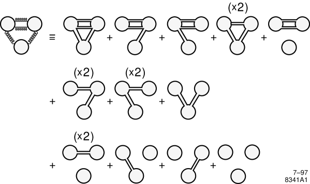
Figure 1: This example illustrates the terminology introduced in the text. This particular “bubble” diagram has $n=4$, $\ell=3$ and decomposes into $2^{4}$ component-diagrams: $(1\times)\,{{\mathcal{D}}_{4,3}^{4}},\,(4\times)\,{{\mathcal{D}}_{4,3}^{3}},\,(6\times)\,{{\mathcal{D}}_{4,3}^{2}},\,(4\times)\,{{\mathcal{D}}_{4,3}^{1}},\,(1\times)\,{{\mathcal{D}}_{4,3}^{0}}$. Some of these component-diagrams are disconnected; this is the case for the last component-diagram of the first row which decomposes into two connected graphs with $2$ loops and $1$ loop, respectively: ${{\mathcal{D}}_{4,3}^{2}}\,={{\mathcal{C}}_{2}^{2}}\times{{\mathcal{C}}_{1}^{0}}$. The index ${\varpi}$ of these component-diagrams are $2,1,1,1,1$ and $1$ for the six contributions of the first row and is $0$ for the remaining $10$ contributions occupying the last three rows. The large-$N_{c}$ limit is controlled by the first diagram with maximal ${\varpi}=2$, while the vanishing-$N_{c}$ limit is dominated by the “tree”-graphs characterized by ${\varpi}=0$.

Having introduced this terminology, we now express the $N_{c}$-dependence of a physical quantity. The color dependence ${{\mathcal{C}}_{n,\ell}}$ of a “bubble” diagram ${{\mathcal{R}}_{n,\ell}}$ is, expressed in terms of ${\widehat{\alpha}_{s}}$ and ${\widehat{n_{f}}}$,

$${{\mathcal{C}}_{n,\ell}} = \,{\widehat{\alpha}_{s}}^{n}\,{\widehat{n_{f}}}^{\ell}\ {\bf\Lambda}^{\ell-n}\sum_{i}^{2^{n}}(-1)^{n-e_{i}}\left(N_{c}^{2}\right)^{{\varpi}_{i}}$$ (17)

$$= \,{\widehat{\alpha}_{s}}^{n}\,{\widehat{n_{f}}}^{\ell}\ {\bf\Lambda}^{\ell-n}\sum_{i}^{2^{n}}(-1)^{n-e_{i}}\ \prod_{\alpha=1}^{d_{i}}\ \left(N_{c}^{2}\right)^{{\varpi}_{i}^{\alpha}}$$

where ${\bf\Lambda}$ is viewed as an analytic function of $N_{c}^{2}$, and we have introduced a topological index ${\varpi}_{i}^{\alpha}$ defined as

$${\varpi}_{i}^{\alpha}=e_{i}^{\alpha}+(\chi_{i}^{\alpha}-\ell^{\alpha}_{i})/2\,.$$ (18)

The total index ${\varpi}_{i}$ for a component-diagram is

$${\varpi}_{i}=\sum_{\alpha}^{d_{i}}{\varpi}_{i}^{\alpha}=e_{i}+(\chi_{i}-\ell)/2\,.$$ (19)

Using Eqs. (17-19) above, we can readily demonstrate all results we inferred from the earlier examples, namely, $(1)$ analyticity in $N_{c}^{2}$ of ${{\mathcal{C}}_{n,\ell}}$, $\,(2)$ “homogeneity” as formulated in Eq. (14), and $(3)$ Abelian behavior in the vanishing $N_{c}\to 0$ limit.

To establish the analyticity of ${{\mathcal{C}}_{n,\ell}}$ as a function of $N_{c}^{2}$ (or ${\bf\Lambda}$), we need only to observe that $(\chi_{i}^{\alpha}+\ell^{\alpha}_{i})/2$ is an integer, $\leq 1$, the equality being satisfied when the corresponding connected graph ${{\mathcal{C}}_{\ell^{\alpha}_{i}}^{e_{i}^{\alpha}}}$ has a planar topology.

In order to establish the two other points, we observe that the index ${\varpi}_{i}$ defined in (19) for each component-diagram ${{\mathcal{D}}_{n,\ell}^{e_{i}}}$ in Eq. (17) is a nonnegative integer (cf. Appendix A). In particular,

1. ${\varpi}_{i}$ is maximal and equal to $n+(\chi_{i}-\ell)/2$ when the component-diagram ${{\mathcal{D}}_{n,\ell}^{e_{i}}}$ is itself connected ($d_{i}=1$) with $e_{i}^{\alpha}=n$, corresponding to replacing all gluons in the “bubble” diagram with “double lines” (See Fig. $1$).

2. ${\varpi}_{i}$ is minimal and zero when each corresponding exponent ${\varpi}_{i}^{\alpha}$ is zero. This case arises when each of the connected graph ${{\mathcal{C}}_{\ell^{\alpha}_{i}}^{e_{i}^{\alpha}}}$ has its $\ell^{\alpha}_{i}$ fermion loops interconnected with “double lines” such that there is no closed path; in particular, there is no more than one “double line” between two fermion loops (See Fig. $1$). An alternate formulation amounts to saying that every corresponding connected graph has a “tree” shape. The “tree”-graph has a planar topology characterized by one face ($F=1$), no handle ($H=0$) and the number of holes equal to the number of fermion loops ($B=\ell$).

We can now proceed further. In order to demonstrate the “homogeneity” rule stated in Eq. (14), we consider the large-$N_{c}$ behavior of Eq. (17).

The large-$N_{c}$ behavior is readily seen to arise from the component-diagram with maximal index ${\varpi}_{i}$, that is, from the connected component-diagram composed of only one connected graph obtained from replacing all gluons with “double lines” as explained in item $(1)$. In that case, ${{\mathcal{C}}_{n,\ell}}$ is a Laurent series in $N_{c}^{2}$ whose leading term is

$$\left.{{\mathcal{C}}_{n,\ell}}\right|_{N_{c}\to\infty}=\,{\widehat{\alpha}_{s}}^{n}\,{\widehat{n_{f}}}^{\ell}\ {c_{\infty}}^{\ell-n}\left(N_{c}^{2}\right)^{(\chi_{\rm max}+\ell)/2}\,.$$ (20)

As noted before, the exponent $(\chi_{\rm max}+\ell)/2$ is $\leq 1$, the equality being achieved for a “bubble” diagram with planar topology, in which case, the physical quantity scales as $N_{c}^{2}\sim{\bf\Lambda}$. This is expected in the context of a membrane interpretation of the color space in the large $N_{c}$ limit, for which physical quantities naturally scale as the area of the membrane, $\propto N_{c}^{2}$ [2]. This fact is also at the origin of the “scaling” law stated in Eq. (14, 15) which is the statement that $\alpha,\beta,\gamma,\ldots$ defined in Eq. (14), satisfy

$$\alpha+\beta+3\gamma+\cdots\,=\,\chi_{\rm max}+\ell\,,$$ (21)

a number fixed by the number of loops $\ell$ and the topology of the “bubble” diagram. The inequality in Eq. (15) translates into the known inequality $\chi+\ell\leq 2$, which saturates only for planar diagrams.

In the vanishing limit ($N_{c}\to 0$), the component-diagrams that dominate the color factor are those which are the most suppressed in the large-$N_{c}$ limit. More precisely, they are those for which the index ${\varpi}_{i}$ is minimal and vanishes. According to item $(2)$ above, this happens for those component-diagrams composed of tree-graphs. The value of the color factor of a “bubble” diagram becomes a polynomial in $N_{c}^{2}$, whose nonvanishing term is

$$\left.{{\mathcal{C}}_{n,\ell}}\right|_{N_{c}\to 0} = \,{\widehat{\alpha}_{s}}^{n}\,{\widehat{n_{f}}}^{\ell}\times{{N_{c}\to 0}\choose{\rm QED}}$$

$$\mbox{with}\qquad{{N_{c}\to 0}\choose{\rm QED}} = \,{c_{0}}^{\ell-n}\sum_{i}^{\rm tree\atop\rm diagrams}\left(-1\right)^{\ell-e_{i}}\,.$$ (22)

The factor ${{N_{c}\to 0}\choose{\rm QED}}$ is the “offset” with respect to the QED value. Setting ${{N_{c}\to 0}\choose{\rm QED}}$ to $1$ formally in Eq. (22) amounts to setting ${\widehat{N_{c}}}\to 0$ and $\widehat{C_{F}},{\widehat{{\left({d_{abc}\over 4}\right)^{2}}}},\ldots\,\to\,1$ in the examples shown earlier and formally reproduces the corresponding QED calculation with ${\widehat{n_{f}}}$ flavors. However, this is not an analytic procedure, since there is no choice of value for ${c_{0}}$ which sets the “offset” ${{N_{c}\to 0}\choose{\rm QED}}$ to $1$ for all diagrams.

The factor ${{N_{c}\to 0}\choose{\rm QED}}$ is very easy to compute for an arbitrary diagram. The calculation is a simple combinatoric exercise which does not make use of the full structure of the original diagram because the sum involved is limited to tree-graphs; we provide some examples in Appendix B. In particular, the non-Abelian structure of the original diagram such as gluon loops and cubic- and quartic-gluon vertices are all suppressed by powers of $N_{c}^{2}$ in the vanishing limit. Furthermore, because the endpoints of a “double line” involved in the “tree”-graphs are each attached to one face, the corresponding generators belong to the Cartan sub-algebra of $SU(N_{c})$. Hence, all remnant of non-Abelianity has vanished in the $N_{c}\to 0$ limit. More precisely,

$$\lim_{N_{c}\to 0}\,SU(N_{c})\ =\ \lim_{N_{c}\to 0}\,\left[U(1)\right]^{N_{c}-1}\,.$$ (23)

This result confirms the change of sign of the first coefficient ${\widehat{\beta}}_{0}$ of the beta-function for sufficiently small values of $N_{c}$. The color factor of a “tree”-graph scales as $N_{c}^{0}$, i.e., it has “dimension” 0. The zero-“dimension” of a “tree”-graph suggests a “point-like” structure which reflects its topological properties, namely $\ell$ punctures on a surface (the number of holes $B=\ell$) interconnected so to form a mesh of zero area (the mesh has no closed loops so that its number of faces is minimal $F=1$). These properties are to be contrasted with the know non-Abelian limit

$$\lim_{N_{c}\to\infty}\,SU(N_{c})\ =\ \lim_{N_{c}\to\infty}\,U(N_{c})\,.$$ (24)

In this limit, the color structure is controlled by planar diagrams of “dimension” $2$ [1, 8], and the natural objects are two-dimensional [2].

A question which comes to mind is what is the dynamics underlying the $N_{c}\to 0$ limit of an $SU(N_{c})$ gauge theory, represented by the expansion (22). To provide a full answer to this question may require the introduction of a prescription to construct the $N_{c}\to 0$ limit of a Feynman diagram with external legs, a mathematical challenge that we haven’t addressed in the present work. One may naively anticipate, however, that the $N_{c}\to 0$ limit is not a quantum field theory defined in the usual sense: The $N_{c}(N_{c}-1)$ off-diagonal gluons disappear from the theory, degrees of freedom which might otherwise be needed to insure unitarity and positivity. The interpretation of the dynamics of the Abelian $N_{c}\to 0$ limit is more likely to take a more geometrical form in light of the point-like nature of this limit on a surface in color space. Along these lines, while the large-$N_{c}$ limit relates the dynamics of certain $SU(N_{c})$ theories to the tension of a membrane [2], the small-$N_{c}$ limit plausibly relates its dynamics to interlinked punctures on a surface. Because these points (fermion loops) are connected pairwise so as not to form a closed path which would otherwise be suppressed by $N_{c}^{2}$, the dynamics of this limit evidently does not depend on the tension of the surface.

It is intriguing to observe from Eq. (14) that the small-$N_{c}$ limit receives contributions from higher order Casimirs of $SU(N_{c})$ at arbitrary $N_{c}$, the number of which increases as $N_{c}$ increases. For example, the cubic Casimir ${(d_{abc}/4)^{2}}$ which arises for $SU(N_{c})$ with integer $N_{c}\geq 3$ and which vanishes for $N_{c}=$ 1 and 2, does contribute to the $N_{c}\to 0$ limit. This relation of the small-$N_{c}$ limit to the algebraic structure of the large-$N_{c}$ limit is an important consequence of the extension of the rescaled group-theoretic objects of $SU(N_{c})$ viewed as an analytic function of $N_{c}^{2}$. This may be indicative of a more profound connection between the large- and small-$N_{c}$ theories.

It is remarkable that a topological expansion determines the color structure of $SU(N_{c})$ in both the large- and the small-$N_{c}$ limits. This observation and the analyticity properties demonstrated above are in our view in strong support of a yet to be uncovered deeper and more universal structure underlying $SU(N_{c})$ gauge theories for arbitrary values of $N_{c}$.

Appendix A

In this appendix, we sketch the proof of the stated properties of the index ${\varpi}_{i}^{\alpha}={e_{i}^{\alpha}+(\chi_{i}^{\alpha}-\ell^{\alpha}_{i})/2}$ defined in (18) which is characteristic of the topology of a connected graph ${{\mathcal{C}}_{\ell^{\alpha}_{i}}^{e_{i}^{\alpha}}}$ composed of $\ell^{\alpha}_{i}$ fermion loops and $e_{i}^{\alpha}$ “double lines”.

All stated properties of the index ${\varpi}$ can be derived from the following rules:

• If two connected graphs ${{\mathcal{C}}_{1}}$, ${{\mathcal{C}}_{2}}$ are interconnected with one “double line”, the newly formed connected graph ${{\mathcal{C}}_{12}}$ satisfies ${\varpi}_{12}={\varpi}_{1}+{\varpi}_{2}$.

• If one “double line” is attached to a connected graph ${{\mathcal{C}}_{1}}$, the new connected graph ${{\mathcal{C}}}$ has an index ${\varpi}={\varpi}_{1}+1$.

• The simplest connected graph composed of one fermion loop and no “double line” has ${\varpi}=0$.

The proof of the above statements rely on the relation $\chi=F-E+V$, where $F$ is the number of faces, $E$, the number of edges and $V$ the number of vertices. The first item above relies on the fact that when adding one “double line”, $F\to F-1$, $E\to E+3$ and $V\to V+2$; similarly for the second item with $F\to F+1$ instead; the last item is a consequence of a fermion loop being characterized by $F=1$ and $E=V=0$.

In order to demonstrate that ${\varpi}\geq 0$, it suffices to observe that all graphs, connected or not, can be constructed from more elementary ones according to the rules above.

Appendix B

In this appendix we illustrate with a few examples the simplicity of the sum over “tree”-graphs in Eq. (22):

$$\left.{\widehat{{\mathcal{C}}_{n,\ell}}}\right|_{N_{c}\to 0} = \,{\widehat{\alpha}_{s}}^{n}\,{\widehat{n_{f}}}^{\ell}\times{{N_{c}\to 0}\choose{\rm QED}}$$

$$\mbox{with}\qquad{{N_{c}\to 0}\choose{\rm QED}} = \,{c_{0}}^{\ell-n}\times\sum_{i}^{\rm tree\atop\rm diagrams}\left(-1\right)^{\ell-e_{i}}\,.$$

Recall that all diagrams with non-Abelian couplings contribute to zero in the small-$N_{c}$ limit. The first nontrivial example is a “bubble” diagram with one fermion loop and an arbitrary number of gluons. The only “tree”-graph is the fermion loop itself with $e_{i}=0$; hence, ${{N_{c}\to 0}\choose{\rm QED}}$ becomes

$${{N_{c}\to 0}\choose{\rm QED}} = \,{c_{0}}^{1-n}\times\sum_{i}^{\rm tree\atop\rm diagrams}\left(-1\right)^{1-e_{i}}$$ (25)

$$= \,{c_{0}}^{1-n}\times\left[\ \ {\bf\bigcirc}\ \ \right]$$

$$= \,{c_{0}}^{1-n}\times\left(\ -1\ \right)\,.$$

As a second example, consider the most general two-fermion loop diagram with $n$ gluons, $p$ of them interconnecting the two loops. For that case, there are two types of “tree”-graphs and one obtains

$${{N_{c}\to 0}\choose{\rm QED}} = \,{c_{0}}^{2-n}\times\sum_{i}^{\rm tree\atop\rm diagrams}\left(-1\right)^{2-e_{i}}$$ (26)

$$= \,{c_{0}}^{2-n}\times\left[\ {\bf\bigcirc}\ {\bf\bigcirc}\ \ +\ p\ {\bf\bigcirc\!\!=\!=\!\!\bigcirc}\ \right]$$

$$= \,{c_{0}}^{2-n}\times\left(\ 1\ -\ p\ \right)\,.$$

Now we consider the most general three-fermion loops diagram with $n$ gluons, each pair of fermion loops being interconnected with $p,q$ and $r$ gluons respectively. For that case there are three topologically distinct types of “tree”-graphs and

$${{N_{c}\to 0}\choose{\rm QED}} = \,{c_{0}}^{3-n}\times\sum_{i}^{\rm tree\atop\rm diagrams}\left(-1\right)^{3-e_{i}}$$ (27)

$$= \,{c_{0}}^{3-n}\times\left[\ {\bf\bigcirc}\ \ {\bf\bigcirc}\ \ {\bf\bigcirc}\right.$$

$$\left.+\ (p+q+r)\ {\bf\bigcirc\!\!=\!=\!\!\bigcirc}\ {\bf\bigcirc}\ +\ (pq+qr+rp)\ {\bf\bigcirc\!\!=\!=\!\!\bigcirc\!\!=\!=\!\!\bigcirc}\ \right]$$

$$= \,{c_{0}}^{3-n}\times\left(\ -1\ +\ (p+q+r)\ -(pq+qr+rp)\ \right)$$

$$= \,{c_{0}}^{3-n}\times\left(\ (p-1)(q-1)(r-1)\ -\ pqr\ \right)\,.$$

This example easily generalizes to $n$ gluons and $\ell$ fermion loops interconnected so to form a ring, i.e., interconnected with $p_{(12)},\ldots,p_{(\ell 1)}$ gluons:

$${{N_{c}\to 0}\choose{\rm QED}}\,=\,{c_{0}}^{\ell-n}\times\left(\ (p_{(12)}-1)\cdots(p_{(\ell 1)}-1)\ -\ p_{(12)}\cdots p_{(\ell 1)}\ \right)\,.$$ (28)

Finally, the most general “bubble” diagram with $\ell$ fermion loops labeled with $i=1,\ldots,\ell$ and $n$ gluons distributed such that $p_{(ij)}$ of them interconnect the fermion loops $i$ and $j$, will have a “offset” factor ${{N_{c}\to 0}\choose{\rm QED}}$ given by the sum

$${{N_{c}\to 0}\choose{\rm QED}} = \,{c_{0}}^{\ell-n}\times\sum_{i}^{\rm tree\atop\rm diagrams}\left(-1\right)^{\ell-e_{i}}$$

$$= \,{c_{0}}^{\ell-n}(-1)^{\ell}\,\times\left[\ {\bf\bigcirc}\ \cdots{\bf\bigcirc}\ +\ (p_{(12)}+\cdots+p_{(ij)}+\cdots)\ {\bf\bigcirc\!\!=\!=\!\!\bigcirc}\ {\bf\bigcirc}\ \cdots{\bf\bigcirc}\right.$$

$$+ \ \left.(p_{(12)}p_{(34)}+\cdots+p_{(ij)}p_{(kl)}+\cdots)\ {\bf\bigcirc\!\!=\!=\!\!\bigcirc}\ {\bf\bigcirc\!\!=\!=\!\!\bigcirc}\ {\bf\bigcirc}\ \cdots\ {\bf\bigcirc}\ +\ \cdots\right]$$

$$= \,{c_{0}}^{\ell-n}(-1)^{\ell}\,\times\left(\ 1\ -\ \sum_{(ij)}p_{(ij)}\,+\,\sum_{(ij)\neq(kl)}p_{(ij)}p_{(kl)}\,-\,\cdots\ \right)\,.$$

Using Eq. (Appendix B) above, one can show that

$$\sum_{i}^{\rm tree\atop\rm diagrams}\left(-1\right)^{\ell-e_{i}}\,\leq\,0\,.$$ (30)

With the help of Eq. (30) one can infer that ${{N_{c}\to 0}\choose{\rm QED}}\leq 0$ when ${\bf\Lambda}(N_{c}\to 0)=-{c_{0}}<0$.

References

- [1] G. t’Hooft, Nucl. Phys. B72 461 (1974), Nucl. Phys. B75 461 (1974).
- [2] J. Hoppe, MIT Ph.D. Thesis, 1982, and in Proc. Int. Workshop on Constraint’s theory and relativistic dynamics, ed. G. Longhi and L. Lusanna (World Scientific, 1987). B. de Witt, J. Hoppe and H. Nicolai, Nucl. Phys. B305 545 (1988).
- [3] L. Susskind, preprint SU-ITP-97-11 (1997), hep-th/9704080.
- [4] M. Mezard, G. Parisi and M. A. Virasoro, “Spin Glass Theory And Beyond”, World Scientific, Singapore (1987) and references therein.
- [5] F. J. Wegner, “Anderson Localization”, edited by H. Nagaoka and H. Fukuyama, Springer, Berlin (1982). P. A. Lee and T. V. Ramakrishnan, Rev. Mod. Phys. 57, (1985).
- [6] P. Cvitanović, Phys. Rev. D14 1536, (1976). Group Theory, P. Cvitanović, p.136 Nordita (1984) .
- [7] M. Engelhardt, Nucl.Phys. B440 543 (1995).
- [8] G. Veneziano, Nucl. Phys. B117 519 (1976).
- [9] M. A. Samuel and L. R. Surguladze, Rev. Mod. Phys. 68 259, (1996). S. G. Gorishny, A. L. Kataev, S. A. Larkin and L. R. Surguladze, Phys. Lett. 256 81 (1991). T. van Ritbergen, J.A.M. Vermaseren and S. A. Larin, preprint UM-TH-97-01, hep-ph/9701390.