Electroweak Baryogenesis Using Baryon Number Carrying Scalars

Abstract

We describe a new mechanism for the generation of the baryon asymmetry of the universe during a first order electroweak phase transition. The mechanism requires the existence of two (or more) baryon number carrying scalar fields with masses and CP violating mixing which vary with the Higgs field expectation value. This mechanism can be implemented using squarks in supersymmetric theories or using leptoquarks. Our central observation is that reflection of these scalars from a bubble wall can yield a significant net baryon number flux into the symmetric phase, balanced by a flux of opposite sign into the broken phase. For generic parameter choices, scalars with incident energies in a specific, but not narrow, range yield order one reflection asymmetries (between the probability of reflection of the scalars and of their antiparticles). The interesting energies are those for which there are two propagating scalars in the symmetric phase but only one in the broken phase. Electroweak sphaleron processes drive the baryon number in the symmetric phase toward zero, but do not act in the broken phase. Our estimate of the resulting baryon asymmetry is consistent with cosmological observations for a range of mass parameters and CP violating phases in a supersymmetric implementation, as long as the bubble walls are not too fast and not too thick.

I Introduction

Understanding how the baryon asymmetry of the universe (BAU) could have arisen from matter–antimatter symmetric initial conditions remains a central challenge at the interface between high energy physics and cosmology. The observed light element abundances, combined with the theory of big bang nucleosynthesis, yield the constraint that the ratio of the cosmological baryon number density to the cosmological entropy density lies in the range $3\times 10^{-11}<n_{B}/s<9\times 10^{-11}$[1]. As has been understood since the work of Sakharov[2], a theory that explains the generation of a net baryon asymmetry must include departures from thermal equilibrium, and must include processes that violate baryon number conservation, charge conjugation symmetry C, and CP symmetry, the product of charge conjugation and parity symmetry P. These conditions can be satisfied by electroweak processes in the early universe, raising the possibility of an electroweak explanation of the BAU[3-28]. In particular, Sakharov’s requirements are all satisfied during a first order electroweak phase transition[7-26]. As the universe cools through the transition temperature $T_{c}$, non-equilibrium conditions exist near the bubble walls that are sweeping through the universe, converting the high temperature “symmetric” phase to the low temperature “broken” phase. Baryon number is violated in the electroweak theory as a consequence of the anomaly[29] in processes in which the sphaleron barrier is traversed[30]. The rate for baryon number violating processes is exponentially small at zero temperature and in the broken phase at the critical temperature $T_{c}$, but not in the symmetric phase[4, 31]. C is maximally violated in the electroweak theory, and CP violation enters via the Cabibbo-Kobayashi-Maskawa (CKM) matrix.

Meeting Sakharov’s conditions, as the minimal standard model does, is necessary for generating a cosmological baryon asymmetry, but need not be sufficient for generating an asymmetry as large as that observed. Indeed, in order to explain the observed BAU, it appears that one needs to extend the standard model for at least two reasons. First, although mechanisms using CP violation from the CKM matrix alone have been constructed[13], they seem to be unable to generate the observed BAU[14]. Hence, CP violation beyond that in the standard model seems to be required. Second, regardless of the mechanism by which baryon number is generated, if it is to survive after the electroweak phase transition, baryon number violating processes must be sufficiently suppressed for $T<T_{c}$. This imposes a lower bound on the expectation value of the Higgs field in the broken phase at $T=T_{c}$[5] which is not satisfied in the standard model with an experimentally allowed Higgs mass. This bound can, however, be satisfied in various extensions of the standard model, including the minimal supersymmetric standard model with one top squark lighter than the top quark[23]; throughout this paper, we will assume that the theory is suitably augmented such that the transition is strongly enough first order that the bound is satisfied. Since the energies that are potentially relevant to electroweak baryogenesis will be increasingly explored in the coming decade by present and planned accelerators, it is of great interest to explore new weak-scale physics that can explain the observed BAU.

In this paper, we introduce a new mechanism for generating the BAU at the electroweak phase transition. Our mechanism requires augmenting the standard model by the addition of (at least) two baryon number carrying complex scalar fields $\phi_{1}$ and $\phi_{2}$ with masses of ${\cal O}(T_{c})$. The two fields must be coupled by off-diagonal terms in their (Hermitian) mass-squared matrix $M^{2}$ which include a CP violating phase. In this way, we introduce CP violation beyond that in the CKM matrix. Furthermore, we require that $M^{2}$ depend upon the Higgs field expectation values in the theory so that the mass eigenvalues and eigenstates are different in the symmetric and broken phases. The requirements just sketched can be implemented in a variety of extensions of the standard model. Perhaps the most appealing possibility is that $\phi_{1}$ and $\phi_{2}$ are the $SU(2)$ singlet and $SU(2)$ doublet top squarks in a supersymmetric extension of the standard model. Another possibility, of interest in light of the recent HERA anomaly[32], is that $\phi_{1}$ and $\phi_{2}$ may be weak-scale leptoquarks whose masses receive contributions from couplings to the Higgs field. Throughout this paper, we focus on the baryogenesis mechanism rather than on model building. For definiteness, however, we present our mechanism and results taking the $\phi$’s to be squarks, and defer discussion of other possibilities to the concluding section.

In a supersymmetric theory, the mass-squared matrix $M^{2}$ depends upon $v_{1}(T)$ and $v_{2}(T)$, the temperature dependent expectation values of the two Higgs doublets $H_{1}$ and $H_{2}$ that give mass to the down and up type quarks, respectively. The off-diagonal terms in $M^{2}$ are in fact zero in the symmetric phase, where $v_{1}=v_{2}=0$. In the broken phase, the off-diagonal terms are complex and therefore CP violating. More generally, we define $\phi_{1}$ and $\phi_{2}$ as the eigenvectors of $M^{2}$ in the symmetric phase, and note that the mass eigenstates in the wall and in the broken phase are linear combinations thereof.

We will be interested in the reflection and transmission probabilities of $\phi$’s incident on the wall from the symmetric phase. Because of the CP violating phases in $M^{2}$, the probability $R_{12}$ for an incident $\phi_{1}$ to be reflected back into the symmetric phase as a $\phi_{2}$ is not the same as $R_{\overline{12}}$, the probability for an incident antiparticle $\bar{\phi}_{1}$ to be reflected as a $\bar{\phi}_{2}$. We will show that this reflection asymmetry $\Delta R\equiv R_{12}-R_{\overline{12}}\,$ results in a net flux of baryon number from the bubble wall into the symmetric phase, compensated by a flux of the opposite sign into the broken phase. Note that the measure of CP violation in the model is the spatial variation of the phase of the off-diagonal terms in $M^{2}$. A spatially constant phase can be rotated away by a spacetime-independent unitary transformation on the $\phi_{i}$; hence the phase must vary spatially if $\Delta R$ is to be nonzero.

The central observation of this paper is that the reflection asymmetry $\Delta R$ can be large, approaching 1, over a broad range of incident energies, if the phase of the off-diagonal term in $M^{2}$ changes by ${\cal O}(1)$ as the bubble wall is traversed from the symmetric phase into the broken phase. As already noted, because of the dependence of $M^{2}$ on $v_{1}$ and $v_{2}$, the eigenvalues of $M^{2}$ vary within the bubble wall. We assume that the larger of the two eigenvalues in the broken phase is greater than the larger of the two eigenvalues in the symmetric phase. This means that there is in general a range of incident energies $E$ such that in the symmetric phase, both eigenvalues of $M^{2}$ are below $E^{2}$, while in the broken phase, there is only one eigenvalue below $E^{2}$. Therefore, there are two propagating modes with energy $E$ in the symmetric phase and only one in the broken phase. Consider a $\phi_{1}$ incident upon the wall from the symmetric phase with an energy in this range. As it begins to penetrate the wall, it evolves into a linear combination of the position-dependent eigenstates of the matrix $M^{2}$. Since only one mode can propagate in the broken phase, there is a position within the wall at which one mode is totally reflected. The reflected mode, upon re-emerging into the symmetric phase, is some linear combination of $\phi_{1}$ and $\phi_{2}$ which includes a significant $\phi_{2}$ component if there is significant mixing. Another way of understanding what is special about the range of energy under discussion is that at each energy in this range, there is one linear combination of incident $\phi_{1}$ and $\phi_{2}$ that is totally reflected. For this reason, both $R_{12}$ and $R_{\overline{12}}$ are generically large, and $\Delta R$ is also large unless the CP violating phase is small. We will refer to this range of incident energies as the “enhanced reflection zone.” By comparison, for incident energies above the enhanced reflection zone, for which there are two propagating modes in both the symmetric and broken phases and throughout the bubble wall, we find that $\Delta R$ is nonzero but is generically many orders of magnitude smaller than one. The width in energy of the enhanced reflection zone is comparable to the amount by which the masses change between the two phases; in the example we present, the width of the enhanced reflection zone is $90$ GeV. In Section II, we present the parametrization of $M^{2}$ appearing in a supersymmetric theory. We then set up the calculation of $\Delta R$, leaving a detailed presentation of the method of calculation to the Appendix. We evaluate $\Delta R$ and explore its dependence on parameters in $M^{2}$.

Standard model quarks also have an enhanced reflection zone, as discussed by Farrar and Shaposhnikov [13], although its width is only of order the strange quark mass. The resulting BAU is small [14], essentially because the light quarks have mean free paths much shorter than their Compton wavelengths. We defer to Section IV a discussion of the suppression due to the finite mean free path of the heavy scalars we employ in our mechanism; the suppression is not severe.

In Section III, we integrate $\Delta R$ against the appropriate thermal distributions for incident $\phi_{1}$’s and $\phi_{2}$’s to obtain the baryon number flux injected into the symmetric phase. If the wall velocity $v_{w}$ is zero, or if the masses of $\phi_{1}$ and $\phi_{2}$ in the symmetric phase are equal, we find that the baryon number flux due to incident $\phi_{1}$’s is cancelled by that due to incident $\phi_{2}$’s. As long as $v_{w}\neq 0$ and the masses in the symmetric phase are not degenerate, we obtain a nonzero baryon number flux. The larger the fraction of the thermal distributions for incident $\phi$’s lying in the enhanced reflection zone, the larger the baryon number flux will be. The final element in the mechanism involves electroweak baryon number violating processes. These drive the baryon number density in the symmetric phase toward zero. Because they do not act in the broken phase, the final result is a net baryon asymmetry of the universe whose magnitude we estimate in Section IV. Our mechanism yields a BAU consistent with observation if the scalars have nondegenerate masses of order $T_{c}$ in the symmetric phase and if the bubble walls are sufficiently thin and slow. We discuss open questions and model implementations in Section V, and note there that an enhanced reflection zone can arise in leptoquark models, and thus is not peculiar to supersymmetric theories.

To close this introduction, we contrast our mechanism with the charge transport mechanism, pioneered by Cohen, Kaplan and Nelson[7, 12], further developed by many authors, and used to estimate the BAU generated during the electroweak phase transition in supersymmetric theories[19,23-26]. Our mechanism can be seen as a modification of the charge transport mechanism. We make explicit comparisons with the results of Huet and Nelson[19] obtained using the charge transport mechanism and find that our mechanism can yield an $n_{B}/s$ consistent with observation for smaller CP violating phases. The central difference is that in our mechanism, we generate a flux of baryon number into the symmetric phase, whereas in the charge transport mechanism a flux of another quantum number, often left-handed baryon number minus right-handed baryon number, is generated. This axial baryon number can be washed out by QCD processes before it has time to bias electroweak baryon number violating processes[15]. Because our mechanism generates a baryon number flux, it is immune to QCD interference of this kind. This contrast is particularly germane in light of the recent demonstration that the rates for the relevant QCD processes are significantly larger than previously expected[33]. Various authors have noted the possibility that a baryon number flux may be generated, but this has always been assumed to be a small effect. This is in fact true for incident energies such that the number of propagating modes is the same on both sides of the bubble wall. For a generic mass-squared matrix $M^{2}$, however, there is a broad region of incident energies in which fewer modes propagate in the broken phase. We observe that this leads to large reflection asymmetries, and consequently to a large baryon number flux into the symmetric phase, yielding an efficient mechanism for generating a BAU consistent with cosmological observations during the electroweak phase transition. We will refer to the electroweak baryogenesis mechanism we propose as the scalar baryon number transport mechanism.

II $M^{2}$, $\Delta R$, and the Enhanced Reflection Zone

We begin this section by presenting the parametrization of $M^{2}$ appropriate when $\phi_{1}$ and $\phi_{2}$ are left- and right-handed top squarks and set the stage for the calculation of $\Delta R$. We then describe the dependence of $\Delta R$ upon the incident energy and upon parameters in $M^{2}$.

As discussed in the introduction, the CP violation that we exploit results from the mixing between two scalars as they traverse the bubble wall separating regions of symmetric and broken phase at $T=T_{c}$. In this background, terms in the potential that couple the baryon number carrying scalars $\phi_{i}$ to the Higgs fields $H_{1}$ and $H_{2}$ give the $\phi_{i}$ spacetime–dependent masses and mixings which can be encoded in a $2\times 2$ Hermitian mass matrix. In a supersymmetric theory, the scalars $\phi_{i}$ are squarks. Top squarks (stops) are the most promising candidates to play the role we envision for the $\phi_{i}$’s because they can be light without violating experimental upper bounds on neutron and electron electric dipole moments (EDMs). Indeed, Cohen, Kaplan, and Nelson have recently advocated supersymmetric models in which CP violating phases are ${\cal O}(1)$, but observable EDMs do not arise because the first and second generation squarks have masses in the tens of TeV[34]. Although it is conceivable that the scalar baryon number transport mechanism could be implemented using first or second generation squarks, it seems likely that stops will yield the largest contribution to the BAU. The stop mass matrix is[35]

$$M^{2}=\left(\begin{array}[]{cc}~{}~{}\tilde{m}_{tR}^{2}+m_{t}^{2}+m_{Z}^{2}\cos 2\beta\left(\frac{2}{3}\sin^{2}\theta_{W}\right){}{}&m_{t}(Ae^{i\varphi_{A}}+\mu e^{i\varphi_{B}}\cot\beta)\\ {}\hfil&{}\hfil\\ m_{t}(Ae^{-i\varphi_{A}}+\mu e^{-i\varphi_{B}}\cot\beta)&~{}~{}\tilde{m}_{tL}^{2}+m_{t}^{2}+m_{Z}^{2}\cos 2\beta\left(\frac{1}{2}-\frac{2}{3}\sin^{2}\theta_{W}\right){}{}\end{array}\right).$$ (4)

Here, $m_{t}=\lambda_{t}v_{2}$ is the top quark mass, $m_{Z}^{2}=g^{2}(v_{1}^{2}+v_{2}^{2})/2$ is the $Z$-boson mass squared, $\tilde{m}_{tR}$ is the soft SUSY-breaking mass for the $SU(2)$ singlet stop, $\tilde{m}_{tL}$ is the soft SUSY-breaking mass for the $SU(2)$ doublet stop, $\tan\beta=v_{2}/v_{1}$ is the ratio of the Higgs field expectation values, $\mu e^{i\varphi_{B}}$ is the (complex) mass in the Higgs potential coupling the two Higgs fields, and $Ae^{i\varphi_{A}}$ is a complex soft SUSY-breaking term. We will see that the scalar baryon number transport mechanism works best if $\tilde{m}_{tL}$ and $\tilde{m}_{tR}$ are both ${\cal O}(T_{c})$ and differ by about 10-30%. Mass differences of this order can arise due to renormalization group evolution down from some high energy scale at which $\tilde{m}_{tL}=\tilde{m}_{tR}$. Indeed, in the models of Ref. [36], $\tilde{m}_{tL}$ and $\tilde{m}_{tR}$ differ by 20%.

During most of the existence of the expanding bubble, its wall can be treated as flat because its radius of curvature is much larger than its thickness, so the mass matrix will depend only upon one spatial direction, which we take to be the $x$ direction. We choose the convention that the region of large negative $x$ is the symmetric phase and that of large positive $x$ is the broken phase. Both $v_{1}$ and $v_{2}$ vary across the bubble wall. A complete calculation of these profiles is beyond the scope of this paper, although a treatment using the resummed one-loop temperature-dependent effective potential is possible[37]. As is conventional, we make a simple choice in terms of a single width parameter, hoping that this captures the essential physics. Following Ref. [24], we choose profiles such that the $v_{i}(x)$ are $x$-independent for $x<-w/2$ and $x>w/2$ and are sinusoids for $-w/2<x<w/2$. That is, we define the profile function

$$p(x)=\left\{\begin{array}[]{ll}0&x\leq-w/2\\ \frac{1}{2}+\frac{1}{2}\sin\left(\frac{\pi\,x}{w}\right)&-w/2<x<w/2\\ 1&x\geq w/2\end{array}\right.$$ (5)

and then for $v_{1}$, we take

$$v_{1}(x)=v_{1}^{0}\,p(x)\ ,$$ (6)

which varies smoothly from zero in the symmetric phase at $x\rightarrow-\infty$ to $v_{1}^{0}$ in the broken phase at $x\rightarrow\infty$. The parameter $w$ characterizes the width of the wall separating the two phases. Although in reality the profiles behave exponentially for $|x|\gg w$, most of the interesting physics happens where $x$ is varying most rapidly and $p(x)$ is as good a parametrization as any. The choice (5) is convenient numerically, as it allows us to impose boundary conditions at $x=\pm w/2$ rather than at larger $|x|$.

It is crucial to our mechanism that $v_{2}/v_{1}$ vary across the bubble wall so that the overall phase of the off-diagonal term in $M^{2}$ is not constant. We take

$$v_{2}(x) = v_{1}(x)\tan\beta(x)$$ (7)

$$= v_{1}(x)\left[p(x)\,\tan\bar{\beta}+\left(1-p(x)\right)\,\tan(\bar{\beta}-\Delta\beta)\right]$$ (8)

so that $\tan\beta(x)$ varies from $\tan(\bar{\beta}-\Delta\beta)$ in the symmetric phase to $\tan\bar{\beta}$ in the broken phase. We will take $\tan\bar{\beta}=2$ in our estimates. Our results do not depend sensitively on this choice. The appropriate choice for $v_{1}^{0}$ in (6) is not $(250~{}{\rm GeV})\cos\bar{\beta}$, the value it takes at $T=0$, but rather the value it takes in the broken phase at $T=T_{c}$. This can be calculated as a function of parameters in specific models, but we will simply use the reasonable estimate $v_{1}^{0}=(2/3)(250~{}{\rm GeV})\cos\bar{\beta}$. (Our results do not depend sensitively on the choice of prefactor.) In order for the baryon asymmetry generated (by any mechanism) during the electroweak phase transition not to be wiped out, $(v_{1}^{0})^{2}+(v_{2}^{0})^{2}$ must be larger than $T_{c}^{2}$. Estimates for $\Delta\beta$ exist in specific models and range from $0.01-0.03$[24, 38] to $0.25$[26], but there are certainly no experimental constraints on this parameter. In order for the overall phase of the off-diagonal terms in $M^{2}$ to vary with $x$, that is, in order for $M^{2}$ to introduce CP violating effects, we must have

$$\Delta\beta \neq 0$$ (9)

$$\Delta\varphi \equiv \varphi_{A}-\varphi_{B}\neq 0\ .$$ (10)

EDM experiments may constrain $\Delta\varphi$ in some models[39], but it has recently been noted[36] that in other models $\varphi_{B}$ is constrained to be small while $\varphi_{A}$ is essentially unconstrained. Any constraints on the CP violating phases are weakened if the first and second generation squarks are heavy. Finally, note that $\varphi_{A}$ can be generation-dependent. Hence, there is no model-independent constraint on $\Delta\varphi$ for third generation squarks.

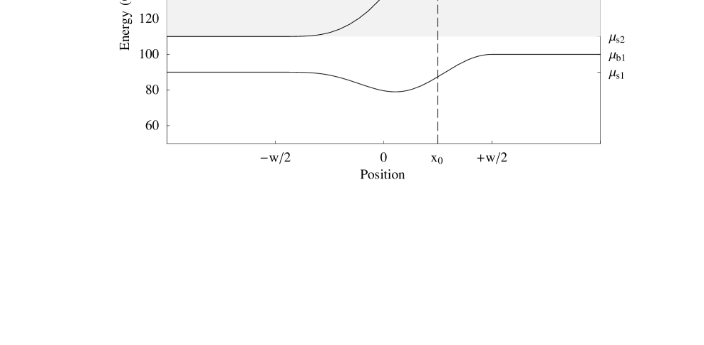
FIG. 1.: Mass eigenvalues as a function of position. The two curves show the square roots of the eigenvalues of $M^{2}$, with parameters given in the text, as a function of $x$. $w$ is the wall width. $\mu_{s1}$ and $\mu_{s2}$ are the mass eigenvalues in the symmetric phase, and $\mu_{b1}$ and $\mu_{b2}$ are the mass eigenvalues in the broken phase. For any incident energy in the shaded range $\mu_{s2}<E<\mu_{b2}$, there is a position $x_{0}$ at which the upper eigenvalue crosses $E$.

As a concrete example which will serve as a visual aid for much of our subsequent discussion, in Figure 1, we plot the eigenvalues of $M^{2}$ as a function of $x$ for the parameter set $\tilde{m}_{tL}=110~{}{\rm GeV}$, $\tilde{m}_{tR}=90~{}{\rm GeV}$, $A=\mu=100~{}{\rm GeV}$, $\tan\bar{\beta}=2$, $\tan(\bar{\beta}-\Delta\beta)=1$, that is $\Delta\beta=0.32$, $\Delta\varphi=\pi/2$, $m_{Z}=91~{}{\rm GeV}$, $m_{t}=175~{}{\rm GeV}$, and $\sin^{2}\theta_{W}=0.23$. With these parameters, the zero temperature masses of the two top squarks are $141~{}{\rm GeV}$ and $243~{}{\rm GeV}$. In our example, we take the wall width to be $w=(4~{}{\rm GeV})^{-1}$. Although the critical temperature $T_{c}$ and the wall velocity $v_{w}$ play no role in the calculation of $\Delta R$, we mention for completeness that when they enter in the next section, we will use $T_{c}=100~{}{\rm GeV}$ and $v_{w}=0.1$ as representative values. It is conventional to write the wall width in terms of the temperature, that is, $w=25/T_{c}$ in our example. Henceforth, we write $T_{c}$ as $T$ when it causes no ambiguity. The final relevant parameter is the $\phi$ mean free path $l$, which will appear in Section IV where we estimate $l\sim 10/T\sim 0.4w$. This completes the enumeration of the parameters specifying the “canonical” example for which we will quote results in the following. We will, of course, describe the effects of varying each of these parameters at appropriate points in the discussion.

We wish to follow a $\phi$ particle from the thermal ensemble in the symmetric phase that last scattered somewhere away from the wall and is now incident upon the wall. Implicit in this scenario is the assumption that the mean free path of the scalars in the plasma is long compared to the wall width $w$. This assumption is likely false, but we nevertheless use it in this section and the next, deferring our treatment of the suppression due to finite mean free paths for the $\phi$ particles to Section IV. The particle impinges upon the wall and is reflected or transmitted, and then resumes its thermal motion in the plasma on one side of the wall or the other. During the time between the last scattering before reflection or transmission and the first after, the particle propagates freely, feeling only the changing expectation values of the Higgs fields which are encoded in the mass matrix. We calculate the reflection coefficients and their asymmetry in the rest frame of the wall; we will boost the resulting baryon number flux to the plasma frame when we calculate it in Section III. In the wall frame, energy is conserved upon traversing the wall since the mass matrix is time-independent. The reflection coefficients can be calculated by solving the time independent Klein-Gordon equations

$$\left[\delta_{ij}(\nabla^{2}+E^{2})-M^{2}_{ij}({\bf x})\right]\phi_{j}({\bf x})=0$$ (11)

because the time dependence of solutions is simply an overall $\exp(iEt)$. In general, we will take a basis in $\phi_{1}$ and $\phi_{2}$ such that far from the wall in the symmetric phase, $M^{2}$ is diagonal. This has already been accomplished, since $\tilde{m}_{tL}^{2}$ and $\tilde{m}_{tR}^{2}$ are the only terms in (4) which are nonzero in the symmetric phase. When calculating the baryon number flux in Section III, we will consider particles incident upon the wall with momenta that are not perpendicular to the wall. However, their reflection coefficients will depend only upon the component of their momentum that is perpendicular to the wall; hence, it suffices to compute reflection coefficients for normal incidence. Therefore, the problem of finding reflection coefficients is effectively a one-dimensional scattering problem, and equations (11) become ordinary differential equations for $\phi_{j}(x)$.

Consider the mass matrix whose eigenvalues are shown in Figure 1. The behavior of the reflection coefficients is qualitatively different for particles incident from the symmetric phase with energies $E<\mu_{s2}$, $\mu_{s2}<E<\mu_{b2}$, and $E>\mu_{b2}$. For $E<\mu_{s2}$, there is only one propagating mode in both the symmetric and the broken phases. In general, we denote the reflection coefficient for a $\phi_{i}$ from the symmetric phase reflected back into the symmetric phase as a $\phi_{j}$ by $R_{ij}$ for particles, and denote the corresponding quantity for antiparticles by $R_{\overline{ij}}$. For $E<\mu_{s2}$, however, the only reflection coefficients are $R_{11}$ and $R_{\overline{11}}$. Since the CPT conjugate of the reflection of $\phi_{1}$ to $\phi_{1}$ is the reflection of $\bar{\phi}_{1}$ to $\bar{\phi}_{1}$, we see that $R_{11}=R_{\overline{11}}$, and there is no reflection asymmetry. Before proceeding to higher energies, note that for a different mass matrix it may be the case that $\mu_{b1}>\mu_{s2}$. In this case, for $E<\mu_{b1}$ there are two propagating modes in the symmetric phase and none in the broken phase, so both $\phi_{1}$ and $\phi_{2}$ must be totally reflected. We now argue that in this circumstance, the reflection coefficients again cannot be CP violating. Unitarity implies that for total reflection,

$$R_{11}+R_{12} = 1$$ (12)

$$R_{\overline{11}}+R_{\overline{12}} = 1$$ (13)

We see that unitarity, together with $R_{11}=R_{\overline{11}}$, implies that $R_{12}=R_{\overline{12}}$ and hence there is no reflection asymmetry. For the rest of this paper, it is implicit that references to $\mu_{s2}$ should be replaced by references to $\mu_{b1}$ if the mass matrix is such that $\mu_{b1}>\mu_{s2}$. We have shown that particles incident from the symmetric phase with energy $E<\mu_{s2}$ yield no reflection asymmetry.

Now consider incident energies $\mu_{s2}<E<\mu_{b2}$, for which there are two propagating modes in the symmetric phase and only one in the broken phase. As shown in Figure 1, for any energy in this shaded range there is a point $x_{0}$ at which the larger eigenvalue of $M^{2}$ equals $E^{2}$. This means that there is a particular linear combination of incident $\phi_{1}$ and $\phi_{2}$ that evolves by mixing as it propagates through the wall in just such a way that upon arrival at $x_{0}$ it is purely in the mass eigenstate with eigenvalue $E^{2}$, and is therefore totally reflected. Since one linear combination of $\phi_{1}$ and $\phi_{2}$ is totally reflected by the wall, both $R_{12}$ and $R_{21}$ are large in this energy range, given sufficient mixing. In order to obtain large asymmetries between the reflection coefficients for particles and for antiparticles, the individual reflection coefficients must of course be large, making this zone of enhanced reflection a promising place to look for large $\Delta R$. Without CP violation, the same linear combination of incident $\bar{\phi}_{1}$ and incident $\bar{\phi}_{2}$ mixes to become the mode with eigenvalue $E^{2}$ at $x_{0}$, and is totally reflected. This implies that $R_{\overline{12}}=R_{12}$ and $R_{\overline{21}}=R_{21}$. However, if the off-diagonal term in $M^{2}$ has a spatially varying phase, then the linear combination of $\bar{\phi}$’s that is totally reflected is different from that for the $\phi$’s, and we expect $\Delta R\neq 0$, as we confirm explicitly below.

Before proceeding, note that $R_{\overline{12}}=R_{21}$ by CPT and therefore

$$\Delta R\equiv R_{12}-R_{\overline{12}}=R_{12}-R_{21}\ .$$ (14)

This simplifies calculations by giving the reflection asymmetry in terms of reflection coefficients for particles only. Another simplification is that in the enhanced reflection zone, $\Delta R$ is the only possible asymmetry because there is no asymmetry due to particles incident from the broken phase. Denoting the single propagating mode in the broken phase by $\phi_{3}$, since $R_{33}=R_{\overline{33}}$ by CPT, unitarity requires that incident $\phi_{3}$’s cannot yield baryon number asymmetric transmission into the symmetric phase. We give a careful explanation of the calculation of $\Delta R$ in the Appendix; henceforth in this section, we focus solely on the results.

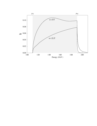
FIG. 2.: $\Delta R$ as a function of incident energy $E$, for two different wall widths $w$. The enhanced reflection zone is shaded.

In Figure 2, we plot $\Delta R$ vs. incident energy $E$ for two values of the wall width, $w=5/T$ and $w=25/T$, with all other parameters as in our canonical example. The enhanced reflection zone is apparent, with $\Delta R\sim 0.1$ for $w=5/T$. Even greater values of $\Delta R$ are obtained for $\Delta\beta$ and $\Delta\varphi$ that are larger than our canonical values. (For example, for $\Delta\beta=1$ and $\Delta\varphi=2.5$, we find $\Delta R\sim 0.3$.) We have therefore confirmed that in the enhanced reflection zone, large reflection coefficients yield large reflection asymmetries in the presence of ${\cal O}(1)$ CP violating phases. For incident energies below the enhanced reflection zone, $\Delta R\equiv 0$. At higher energies, that is for $E>\mu_{b2}$, there are two propagating modes in both the symmetric and the broken phases and throughout the wall. In this regime, $\Delta R\neq 0$, but it is extremely small. For $w=5/T$, $\Delta R=0.0047$ at $E=200~{}{\rm GeV}$; $\Delta R=2.5\times 10^{-5}$ at $E=250~{}{\rm GeV}$; and $\Delta R=1.3\times 10^{-6}$ at $E=300~{}{\rm GeV}$. For these energies, transmission coefficients are very close to $1$ and reflection coefficients (and therefore $\Delta R$) are very small.

For energies above $\mu_{b2}$, unlike for those in the enhanced reflection zone, there is the possibility of a nonzero asymmetry arising from particles and antiparticles incident from the broken phase and transmitted through the wall into the symmetric phase. This asymmetry is very small, as we now argue. Just as the $R_{ij}$ are very small in this energy range, the reflection coefficients for reflection of particles incident from the broken phase back into the broken phase are very small also. Since any asymmetry associated with transmission into the symmetric phase must be balanced by an asymmetry in reflection, we conclude that even though the transmission coefficients are $\sim 1$, their asymmetry is very small.

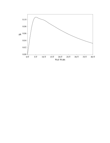
FIG. 3.: $\Delta R$ as a function of wall width $w$ for incident energy $E=150~{}{\rm GeV}$, which is within the enhanced reflection zone.

We now discuss the dependence of $\Delta R$ on the parameters in the problem, beginning with the wall width $w$. Note that in order to obtain a nonzero $\Delta R$, there must be some region in $x$ in which modes incident from the symmetric phase can mix, and hence feel the effects of the CP violating terms, before arriving at $x_{0}$ where one mode is totally reflected. This implies that $\Delta R=0$ for an infinitesimally thin (step function) wall. In the thin wall limit, $R_{12}$ and $R_{\overline{12}}$ are large in the enhanced reflection zone, but they are equal. In Figure 3, we plot $\Delta R$ at $E=150~{}{\rm GeV}$ versus the wall width $w$ for our canonical $M^{2}$. We see that $\Delta R\sim w$ for $w$ small relative to the inverse mass scales in the problem. At large $w$, the number of wavelengths per wall width grows and therefore $R_{12}$ and $R_{\overline{12}}$ decrease, and so does $\Delta R$. The asymmetry $\Delta R$ peaks at about $w=5/T$, one of the values we have chosen to plot in Figure 2. This is an unphysically thin wall — estimates for $w$ range from $10/T$ to $100/T$. (The physics determining $w$ is presented, for example, in Refs. [40, 41].) In our canonical example we follow Ref. [24] and use $w=25/T$, and we have plotted $\Delta R$ for this wall width in Figure 2. If $w$ is in fact smaller than $25/T$, our final result for the BAU is enhanced, while for thicker walls, it is somewhat suppressed.

Let us now consider the effects of varying the mass parameters in $M^{2}$. We define $m$ and $\Delta m$ through

$$\mu_{s1}=\tilde{m}_{tR} = m-\frac{\Delta m}{2}$$ (15)

$$\mu_{s2}=\tilde{m}_{tL} = m+\frac{\Delta m}{2}\ .$$ (16)

For simplicity, we will always take $\mu=A$ and $\tan\bar{\beta}=2$. (The optimal choice for $\bar{\beta}$ should be such that $A\sim\mu\cot\bar{\beta}$. We find, however, that for $A=\mu$, varying $\bar{\beta}$ from 0.5 to 4 changes our results by at most 10%, so the dependence on $\bar{\beta}$ is not significant.) We have investigated the dependence of our results on $m$, $\Delta m$ and $A$. Of course, we do not vary the $m_{Z}^{2}$ and $m_{t}^{2}$ terms in $M^{2}$, and these should be thought of as setting the energy scale. Varying $m$ between $50$ and $150~{}{\rm GeV}$ while holding $\Delta m/m$ and $A$ fixed changes $\Delta R$ by less than 20%. Increasing $m$ further leads to a suppression of $\Delta R$ because it increases all the eigenvalues relative to $1/w$. For $A=0$, there is no mixing between $\phi_{1}$ and $\phi_{2}$, and $\Delta R=0$. Increasing $A$ from $0$ to $200~{}{\rm GeV}$ holding all else fixed yields a monotonically increasing $\Delta R$, but in going from $A=100~{}{\rm GeV}$ to $A=200~{}{\rm GeV}$, the increase in $\Delta R$ is less than 10%. Of the three mass parameters we have varied, $\Delta m$ has the biggest effect. $\Delta R$ is maximized for $\Delta m=0$. However, we will see in the next section that the baryon number flux is identically zero for $\Delta m=0$. As $\Delta m$ is increased, $\Delta R$ falls; by a few percent at $\Delta m/m=0.2$; by about a factor of two at $\Delta m/m=0.8$. We defer a plot displaying the dependence of our results on $\Delta m$ to the next section.

Finally, we come to the CP violating phase. We have verified that for small $\Delta\varphi$ and $\Delta\beta$, $\Delta R$ is linear in both quantities. As we have noted, there is no model-independent constraint on $\Delta\varphi$; therefore, in Figure 4 we show $\Delta R$ over the entire range of $\Delta\varphi$. We see that $\Delta R$ is approximately linear in $\Delta\varphi$ for $|\Delta\varphi|\leq 2$. We find that $\Delta R$ is linear in $\Delta\beta$ over the range $-0.2<\Delta\beta<0.5$. The values we have been using in our canonical example — $\Delta\varphi=\pi/2$ and $\Delta\beta=0.32$ — are within the linear regime. For convenience, in subsequent sections, we often quote results assuming that $\Delta\beta$ and $\Delta\varphi$ are in their linear regimes, as is likely the case for $\Delta\beta$, but not necessarily for $\Delta\varphi$. Fortified by our understanding of how $\Delta R$ in the enhanced reflection zone varies with wall width, masses, and phases, we are ready for the next step in our computation of the BAU.

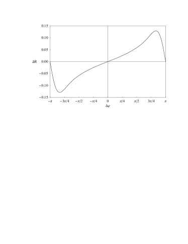
FIG. 4.: $\Delta R$ as a function of $\Delta\varphi$ for incident energy at the center of the enhanced reflection zone.

III From Asymmetric Reflection Coefficients to Baryon Number Flux

We now compute the baryon number flux into the symmetric phase by integrating $\Delta R$ against the flux densities of the incident particles. The flux, which we denote by ${\cal F}_{B}$, receives two contributions. One contribution, $F_{s\to s}$, is generated by the asymmetry in the reflection of particles and antiparticles incident on the wall from the symmetric phase and is associated with $\Delta R$. The other contribution, $F_{b\to s}$, is caused by the asymmetry in the transmission of the particles and their antiparticles incident on the wall from the broken phase. We have seen, however, that this asymmetry (unlike $\Delta R$) is zero for energies in the enhanced reflection zone, and is small (like $\Delta R$) at higher energies. We therefore neglect $F_{b\to s}$ and obtain

$${\cal F}_{B}\simeq\frac{1}{3}F_{s\to s}\ .$$ (17)

The factor of 1/3 arises because the $\phi$ particles have baryon number 1/3.

Before deriving an expression for $F_{s\to s}$, we make some general observations. The processes we are studying are invariant under time translations (although not under time reversal!). Therefore, energy is conserved upon reflection from or transmission through the wall. We denote the components of a particle’s momentum in the rest frame of the wall that are perpendicular and parallel to the wall by $p_{i\perp}$ and ${\vec{p}_{i\parallel}}$, respectively. Recalling that $M^{2}$ is diagonal in the symmetric phase, we have

$$E^{2}=p_{1\perp}^{2}+p_{1\parallel}^{2}+\mu_{s1}^{2}=p_{2\perp}^{2}+p_{2\parallel}^{2}+\mu_{s2}^{2}\ ,$$ (18)

where $p_{i\parallel}=|{\vec{p}_{i\parallel}}|$. Since the processes of reflection from and transmission through the wall are invariant under spatial translations in the directions parallel to the wall, $\vec{p}_{i\parallel}$ is conserved. For example, for a $\phi_{1}$ reflecting into a $\phi_{2}$, ${\vec{p}_{1\parallel}}={\vec{p}_{2\parallel}}$. Equation (18) then yields

$$p_{1\perp}^{2}+\mu_{s1}^{2}=p_{2\perp}^{2}+\mu_{s2}^{2}\equiv\varepsilon_{\perp}\ ,$$ (19)

defining a conserved quantity $\varepsilon_{\perp}$. We now see how to translate results obtained in the $(1+1)$-dimensional treatment of the previous section into the full $(3+1)$-dimensional setting appropriate here. What was called $E$ in previous sections is in fact $\varepsilon_{\perp}$. $\Delta R$ depends on $\varepsilon_{\perp}$, and the enhanced reflection zone is given by $\mu_{s2}<\varepsilon_{\perp}<\mu_{b2}$.

Before the arrival of the wall, the $\phi$’s are in thermal equilibrium with momenta distributed according to the Bose-Einstein distribution. This equilibrium distribution defines a rest frame, the plasma frame, which is different from the rest frame of the wall. In order to compute ${\cal F}_{B}$, we need the flux density of $\phi_{i}$ particles (equivalently, $\bar{\phi}_{i}$ antiparticles) incident upon the wall with a given momentum in the wall frame. Throughout this section, we continue to assume that the mean free path of particles is larger than the wall width, deferring the discussion of the effects of the falseness of this assumption to Section IV. Hence, the incident flux density we require is given simply by

$$f_{i}(E,p_{i\perp})={3p_{i\perp}/E\over e^{\gamma(E-v_{w}p_{i\perp})/T}-1},$$ (20)

where $\gamma\equiv 1/\sqrt{1-v_{w}^{2}}$. The factor of 3 appears because there are $\phi$’s with each of 3 different colors in thermal equilibrium. The argument of the exponential arises because, as mentioned before, the particles are initially in thermal equilibrium in the plasma frame, not in the wall frame. To get $F_{s\to s}$, we must integrate $\Delta R\equiv R_{12}-R_{\overline{12}}=R_{12}-R_{21}$ against $f_{1}$ over the three-momentum of the incident $\phi_{1}$ and integrate $R_{21}-R_{\overline{21}}=R_{21}-R_{12}=-\Delta R$ against $f_{2}$ over the three-momentum of the incident $\phi_{2}$ and add up the results. Thus, we obtain

$$F_{s\to s} = {1\over\gamma}\Bigg{[}\int_{0}^{2\pi}\int_{0}^{\infty}{d\theta\,dp_{1\parallel}\,p_{1\parallel}\over(2\pi)^{2}}\int_{p_{1\perp{\rm min}}}^{\infty}{dp_{1\perp}\over 2\pi}\,\Delta R(p_{1\perp})\,f_{1}(E,p_{1\perp})\Bigg{]}$$ (21)

$$- {1\over\gamma}\Bigg{[}\int_{0}^{2\pi}\int_{0}^{\infty}{d\theta\,dp_{2\parallel}\,p_{2\parallel}\over(2\pi)^{2}}\int_{p_{2\perp{\rm min}}}^{\infty}{dp_{2\perp}\over 2\pi}\,\Delta R(p_{2\perp})\,f_{2}(E,p_{2\perp})\Bigg{]},$$ (22)

where $p_{i\perp{\rm min}}$ is the $p_{i\perp}$ such that $\varepsilon_{\perp}=\mu_{s2}$. Note that $F_{s\to s}$ is the flux seen in the plasma frame. Transforming from the wall frame back to the plasma frame yields the overall factor of $1/\gamma$ in (22). Upon performing the integration over $p_{i\parallel}$, we obtain

$${\cal F}_{B}\simeq\frac{1}{3}F_{s\to s}={T\over 4\pi^{2}\,\gamma^{2}}\int_{\mu_{s2}}^{\infty}d\varepsilon_{\perp}\,\,\varepsilon_{\perp}\,\Delta R(\varepsilon_{\perp})\ln\left[{1-e^{-\gamma(\varepsilon_{\perp}-v_{w}p_{2\perp})/T}\over 1-e^{-\gamma(\varepsilon_{\perp}-v_{w}p_{1\perp})/T}}\right],$$ (23)

where we have used (19) in the form $\varepsilon_{\perp}d\varepsilon_{\perp}=p_{1\perp}dp_{1\perp}=p_{2\perp}dp_{2\perp}$.

From (23), we deduce that $F_{s\to s}=0$ for $v_{w}=0$. This is to be expected, since baryogenesis requires out of equilibrium conditions, and hence requires $v_{w}\neq 0$. (Note that one can derive an expression for $F_{b\to s}$ similar to that for $F_{s\to s}$ and show that $F_{b\to s}=0$ when $v_{w}=0$.) The vanishing of ${\cal F}_{B}$ with $v_{w}$ can be more directly understood as follows. We present the argument in $1+1$ dimensions; the generalization to $3+1$ is trivial. We have shown that $R_{12}-R_{\overline{12}}=-(R_{21}-R_{\overline{21}})$. For $v_{w}=0$, the number of $\phi_{1}$ particles incident upon the wall with an energy $E$ greater than $\mu_{s2}$ is equal to the number of incident $\phi_{2}$ particles with the same energy. (There are of course $\phi_{1}$ particles with $\mu_{s1}<E<\mu_{s2}$, but they do not yield a reflection asymmetry.) Therefore, for $v_{w}=0$, the contribution to ${\cal F}_{B}$ due to incident $\phi_{1}$’s is exactly cancelled by that due to incident $\phi_{2}$’s. Now consider a moving wall, where $v_{w}\neq 0$. $\phi_{i}$ particles incident upon the wall with a given energy $E$ in the wall frame have energy $(E-v_{w}p_{i\perp})$ in the plasma frame, in which they are initially in a thermal equilibrium distribution. If $\mu_{s1}\neq\mu_{s2}$ then $p_{1\perp}\neq p_{2\perp}$ for a given $E$, and the number of $\phi_{1}$ and $\phi_{2}$ particles with incident energy $E$ in the wall frame is not the same. We see that in order to upset the cancellation between the contribution to ${\cal F}_{B}$ due to incident $\phi_{1}$’s and that due to $\phi_{2}$’s, we need both $v_{w}\neq 0$ and $\mu_{s1}\neq\mu_{s2}$. The asymmetry in the reflection coefficients can only yield an asymmetry in the baryon number flux if the wall is moving and if the scalars are not degenerate in mass in the symmetric phase.

As discussed in the previous section, $\Delta R$ depends on parameters in $M^{2}$ and on the wall width. The flux ${\cal F}_{B}$ depends on these parameters as well as on the wall velocity and temperature. We will be interested in the regime in which $v_{w}$ and $\Delta m/m$ are small compared to $1$. This may seem surprising, given that we have just argued that ${\cal F}_{B}$ is zero for $v_{w}\rightarrow 0$ or $\Delta m/m\rightarrow 0$. The reason is that, as we have seen in the previous section, $\Delta R$ is a decreasing function of $\Delta m$ and, as we will see in the next section, the BAU is proportional to ${\cal F}_{B}/v_{w}^{3}$ for realistic wall velocities. In order to gain intuition about (23) it is useful to pretend that $\Delta R$ is energy independent for $\mu_{s2}<\varepsilon_{\perp}<\mu_{b2}$, and then expand in $v_{w}$ and $\Delta m/m$ to first order in both, obtaining

$$\frac{{\cal F}_{B}}{T^{3}}\sim\frac{1}{4\pi^{2}}\,v_{w}\,\frac{\Delta m}{m}\,\left(\frac{m}{T}\right)^{2}\,\Delta R\,\int_{m/T}^{\mu_{b2}/T}\frac{y\,dy}{\left[e^{y}-1\right]\sqrt{y^{2}-(m/T)^{2}}}\ .$$ (24)

We perform all our calculations using (23), not the expansion (24), but the expansion is useful for understanding the qualitative dependence of ${\cal F}_{B}$ on the parameters.

With all parameters as in our canonical example, (23) yields

$$\frac{{\cal F}_{B}}{T^{3}}\sim 9\times 10^{-6}\ ,$$ (25)

and with $w=5/T$ instead of $25/T$, we obtain a result which is a factor of two larger. We have verified that ${\cal F}_{B}$ is linear in $v_{w}$ to within a few percent for $v_{w}<0.6$. In the regime in which ${\cal F}_{B}$ is linear in $\Delta\beta$, $\Delta\varphi$, and $v_{w}$, (25) becomes

$$\frac{{\cal F}_{B}}{T^{3}}\sim 2\times 10^{-4}\,v_{w}\,\Delta\beta\,\Delta\varphi\ .$$ (26)

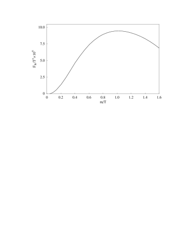
FIG. 5.: Temperature dependence of the baryon number flux. In this plot, $T$ varies and $w=25/T$ for all $T$. We keep all parameters except $T$ and $w$ fixed. We plot ${\cal F}_{B}/T^{3}$ vs. $m/T$ to facilitate comparison with (24).

Turning now to the temperature dependence, in Figure 5, we plot ${\cal F}_{B}/T^{3}$ vs. $m/T$, varying $T$ and keeping all parameters in the mass matrix fixed. Since $\Delta R$ does not depend on $T$, we can partially understand this plot by noting that in (24) ${\cal F}_{B}/T^{3}\sim(m/T)^{2}$ at small $m/T$ and $\sim\exp(-m/T)$ at large $m/T$. This does not completely describe the Figure, however, because as we vary $T$, we have kept $w=25/T$; this means that $w$ changes with respect to the parameters in the mass matrix. We conclude from Figure 5 that the BAU generated by the scalar baryon number transport mechanism is largest for $m\sim T$.

FIG. 6.: Dependence of the baryon number flux on $\Delta m/m$, with $\Delta m$ varying and all other parameters fixed.

In Figure 6, we plot ${\cal F}_{B}/T^{3}$ vs. $\Delta m/m$. It is linear in $\Delta m/m$ for small $\Delta m/m$ and falls at large $\Delta m/m$ because, as we noted in the previous section, $\Delta R$ decreases with increasing $\Delta m/m$. We see that using $\Delta m/m=0.2$ as in our canonical example yields a reasonable estimate for $\Delta R$ over the range $0.1<\Delta m/m<0.3$, but for $\Delta m/m$ outside this range, the BAU is suppressed. For the scalar baryon transport mechanism to be efficient, we need scalars with symmetric phase masses of ${\cal O}(T_{c})$ that differ by 10-30%.

IV Estimating the Baryon Number of the Universe

In the preceding sections, we have shown how to calculate the baryon number flux ${\cal F}_{B}$ carried by $\phi$ particles that is injected into the symmetric phase by the motion of the bubble wall. To this point, we have described the quantitative solution of a well-posed problem. Given a mass matrix, a critical temperature, a wall profile, a wall velocity, and making the assumption that the $\phi$ mean free path is long compared to the wall width, a quantitative calculation of ${\cal F}_{B}$ is attainable. In this section, we sketch a qualitative estimate of the cosmological baryon to entropy ratio, $n_{B}/s$, that results from the flux ${\cal F}_{B}$. Our treatment is admittedly crude and can be improved, for example along the lines of that of Huet and Nelson [19], but we leave this for future work. We organize the estimate of the final result as follows. First, we estimate the mean free path $l$ and the suppression of ${\cal F_{B}}$ that results from the finiteness of $l/w$. Then, we estimate the scalar baryon number density (baryon number in the form of $\phi$’s) that results from ${\cal F}_{B}$. This in turn leads to a quark baryon number density which biases the electroweak sphaleron processes acting in the symmetric phase, resulting in a net baryon asymmetry of the universe.

Before the wall arrives, the $\phi$’s in the symmetric phase are diffusing about with a mean free path in the $x$ direction which we call $l$ and a mean velocity in the $x$ direction between scatterings which we call $v_{\phi}$. The one-dimensional diffusion constant is defined as

$$D=l\,v_{\phi}\ .$$ (27)

The mean one-dimensional velocity is $v_{\phi}\sim 0.7$ for particles with $m=T$. Joyce, Prokopec, and Turok[16] have estimated that in the symmetric phase, the diffusion constant for relativistic strongly interacting particles is $D\sim 6/T$. Most of the scatterings contributing to $D$ are interactions with gluons in the plasma, and $D$ is inversely proportional to the relevant interaction cross-section which decreases with increasing $m$. This suggests that for $m=T$, the diffusion constant is somewhat greater than $6/T$, but we leave a complete calculation for future work. In this paper, we simply use the conservative estimate

$$l\sim\frac{10}{T}\ .$$ (28)

Note that an increase in $m/T$ leads to an increase in $l$, and potentially to a larger final result. Of course, in increasing $m/T$, one pays a penalty in the exponential suppression in (24), and we will see below that making the $\phi$’s nonrelativistic exacts other costs as well.

We now give a crude estimate of the suppression due to the finiteness of $l/w$. As noted in Section II, estimates for $w$ range from $10/T$ to $100/T$. In our canonical example, we use $w=25/T$, yielding $l/w\sim 0.4$. The essence of the effect is that when $\phi$ particles reach $x_{0}$, the point in the wall at which one mode is totally reflected, they have only been travelling (and mixing) freely for a distance of order $l$. To incorporate this, we redo the calculation of $\Delta R$ as follows. For each incident energy, we find $x_{0}$ and choose as incident states the mass eigenstates a distance $l$ to the left of $x_{0}$. These then propagate only a distance $l$ before reflecting, and so experience less $CP$ violating mixing than in the case where $l$ is infinite. The result is a suppression in $\Delta R$ at each energy. We in fact find that this suppression is rather energy dependent, being larger for energies close to $\mu_{b2}$. In evaluating ${\cal F}_{B}$, therefore, we must re-evaluate the integral (23).

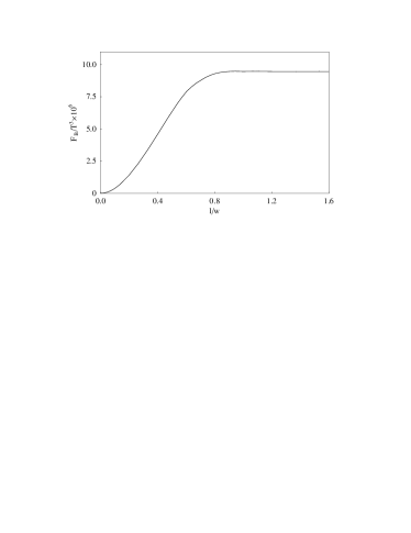
FIG. 7.: Dependence of the baryon number flux on $l/w$, with $l$ varying and all other parameters fixed.

The result is shown in Figure 7, in which we plot ${\cal F}_{B}/T^{3}$ vs. $l/w$. We see that for $l/w=0.4$, the flux ${\cal F}_{B}$ is suppressed by about a factor of $2$ relative to that for infinite $l$. We have also verified that the reflection asymmetries at a given energy are largely insensitive to the form of the potential beyond the corresponding $x_{0}$. Although our method of including the effects of a finite mean free path is certainly not the final word, it should give a reasonable estimate of the magnitude of the suppression. Note in particular that the integrand in (23) is largest for lower energies within the enhanced reflection zone. For these energies, $x_{0}$ is on the symmetric phase side of the wall, and the dependence on $l/w$ is not severe. This qualitative explanation is consistent with our result that ${\cal F}_{B}$ is only suppressed by a factor of 2 for $l/w=0.4$.

If $l$ is larger than we have estimated, as for example would be the case for more non-relativistic $\phi$’s for which $D$ is larger and $v_{\phi}$ is smaller, then the final result could be larger than that which we estimate by up to a factor of $2$. If, on the other hand, $w$ is larger than $25/T$, the final result will be suppressed both by the effect of $wm$ displayed in Figure 3 and by the effect of $l/w$ displayed in Figure 7. Of course, $w<25/T$ would correspondingly enhance the final result, for example by a factor of 4 for $w=l=10/T$. In the estimates that follow, we take ${\cal F_{B}}/T^{3}\sim 5\times 10^{-6}$, as appropriate for $m=A=\mu=T=100{\rm GeV}$, $\Delta m/m=0.2$, $w=25/T$, $l/w=0.4$, $v_{w}=0.1$ and $\Delta\beta\Delta\varphi=0.5$. In the regime in which ${\cal F_{B}}$ is linear in $v_{w}$, $\Delta\beta$, and $\Delta\varphi$, we can write it as

$$\frac{{\cal F}_{B}}{T^{3}}\sim 1\times 10^{-4}\,v_{w}\,\Delta\beta\,\Delta\varphi\ .$$ (29)

The dependence on the other parameters is more complicated, as we have discussed and illustrated above.

Next, we give an estimate of the baryon number density carried by $\phi$ particles in the region in front of the bubble wall. A $\phi$ particle emerging into the symmetric phase from the wall begins to diffuse, and the mean distance such particles have travelled from the wall a time $t$ after being reflected is $x\sim\sqrt{2lv_{\phi}t}$. In the same time $t$, the wall itself has moved a distance $v_{w}t$. Defining $\tau$ as the time that a reflected $\phi$ particle spends in the symmetric phase before the wall overtakes it, we find that on average,

$$\tau\sim\frac{2lv_{\phi}}{v_{w}^{2}}\ .$$ (30)

Note that this means that on average a reflected $\phi$ particle undergoes

$$N_{\rm scatt}\sim\frac{\tau}{l/v_{\phi}}\sim 2\,\left(\frac{v_{\phi}}{v_{w}}\right)^{2}$$ (31)

scatterings during the time $\tau$ it spends in the broken phase. Our treatment is only consistent for $N_{\rm scatt}>1$, and our final result is largest for large $N_{\rm scatt}$. As mentioned above, although non-relativistic $\phi$’s have benefits, they also have costs, and we see one here.

We denote the mean separation between the diffusing particle and the oncoming wall during the time the particle is in the broken phase by $\Delta x$. This quantity will cancel in the final result. Over a range of $x$ in front of the wall given approximately by $\Delta x$, there is a net baryon number density carried by $\phi$ particles given by

$$n_{B}^{\phi}\sim{\cal F}_{B}\,\frac{\tau}{\Delta x}\ .$$ (32)

We arrive at this estimate by noting that ${\cal F}_{B}$ is the baryon number injected into the symmetric phase per unit wall area per unit time and that at any given time, the $\phi$’s reflected in the previous $\tau$ are in a region of order $\Delta x$ ahead of the wall. Thus, we conclude that every point in the universe experiences a baryon density in $\phi$ particles given by (32) for a time

$$t^{*}\sim\Delta x/v_{w}$$ (33)

while in the symmetric phase. By this point, it should be becoming clear that $n_{B}/s$ will turn out to be largest for small wall velocities. The authors of Refs. [40, 41] discuss wall velocities ranging from $0.02$ to $0.4$, and other authors have considered velocities as high as $0.9$. The mechanism we are proposing will be most effective at the lower end of this range, and we have been using $v_{w}\sim 0.1$ in our canonical example. Note also that we are assuming that $n_{B}^{\phi}/T^{3}$ is small, and hence we are not including the effect of the baryon number asymmetry in the distribution functions used in the calculation of ${\cal F}_{B}$ in the previous section.

The mechanism that generates the baryon number flux carried by $\phi$ particles into the symmetric phase does not involve any baryon number violation. Therefore, the baryon number associated with $n^{\phi}_{B}$ must be exactly cancelled by a baryon number of opposite sign behind the wall. Note that the $\phi$ particles, being scalars, are not produced anomalously in electroweak sphaleron processes, and therefore cannot bias such processes. Thus, if this were the end of the story, we would have made no progress. However, $\phi$ particles can be converted into quarks. This is a model-independent statement, equivalent to the statement that the $\phi$’s have baryon number $1/3$. The rate for $\phi$–quark conversion is, however, model dependent. In the supersymmetric case we are using as an example, if the gluino mass $M_{\tilde{g}}$ is less than $\mu_{s2}$, the symmetric phase mass of the heavier squark, then the squarks can decay into gluinos and quarks, since the quarks are massless in the symmetric phase. We will not assume that the gluinos are this light, however. The first process we consider is scattering off a gluino in the thermal bath: squark $+$ gluino $\rightarrow$ quark $+$ gluon. The rate for this process is suppressed relative to that for squark-gluon scattering by $\exp(-M_{\tilde{g}}/T)$ due to the paucity of gluinos in the plasma. It is also suppressed by $(T/M_{\tilde{g}})^{2}$ in the cross-section. The second process we consider is gluon $+$ squark $\rightarrow$ quark $+$ virtual gluino, where the gluino becomes quark $+$ anti-squark or anti-quark $+$ squark. This rate is suppressed relative to ordinary quark-gluon scattering by of order $\alpha_{s}(T/M_{\tilde{g}})^{2}$, and by three-body phase space. Defining $1/b$ as the fraction of scatterings incurred by a $\phi$ particle in the symmetric phase that turn the $\phi$ into a quark, we estimate that $b\sim 200$ for $M_{\tilde{g}}\sim 300~{}{\rm GeV}$, noting again that this estimate is quite model dependent. We can now estimate that the baryon number density carried by quarks in the region $\Delta x$ in front of the wall is

$$n^{q}_{B}\sim n^{\phi}_{B}\,\frac{N_{\rm scatt}}{b}\sim n^{\phi}_{B}\,\frac{2\,v_{\phi}^{2}}{b\,v_{w}^{2}}\ ,$$ (34)

where we have used (31). This estimate is only valid for $N_{\rm scatt}/b<1$; if $N_{\rm scatt}/b>1$ then the squark–quark conversion reactions have time to establish chemical equilibrium, and an analysis in terms of chemical potentials should be used. For $N_{\rm scatt}/b\sim 1$, which is relevant for $M_{\tilde{g}}\sim 300~{}{\rm GeV}$ and $v_{w}\sim 0.1$, the average $\phi$ is converted to a quark at some point during its $N_{\rm scatt}$ scatterings, which leads us to estimate that the baryon number density in quarks is

$$n^{q}_{B}\sim\frac{n^{\phi}_{B}}{2}\sim{\cal F_{B}}\frac{\tau}{2\Delta x}\ ,$$ (35)

where we have used (32). The density $n^{q}_{B}$ does bias electroweak sphaleron processes. Note that a baryon number density in front of the wall cannot be affected by non-perturbative QCD processes. This is in contrast to what happens in many other mechanisms. For example, if an axial baryon number density (more left handed quarks than right handed ones; no net excess of baryons) is generated, this can bias electroweak sphaleron processes only if it is not first wiped out by QCD processes.

The rate per unit volume of baryon number violating sphaleron processes in the symmetric phase is conventionally written as

$$\Gamma_{s}\sim\kappa\alpha_{W}^{4}T^{4}\ .$$ (36)

Recent work[42] shows that $\kappa$ is parametrically ${\cal O}(\alpha_{W})$. The most complete numerical simulations done to date[43] suggest $\kappa=(29\pm 6)\alpha_{W}$. In thermal equilibrium, no net baryon asymmetry is generated by these processes, since sphaleron and “anti-sphaleron” processes occur at the same rate. However, in a region with a nonzero $n_{B}^{q}$, the sphaleron processes tend to reduce the baryon number density. In particular[28]

$$\dot{n}_{B}\sim-\,6\,n_{B}^{q}\,\frac{\Gamma_{s}}{T^{3}}\ .$$ (37)

Assuming that $\Gamma_{s}t^{*}/T^{3}<1$, which is certainly the case for $v_{w}>0.005$, then the net change in $n_{B}$ due to anomalous electroweak processes is

$$\Delta n_{B}=-\,6\,n_{B}^{q}\,\frac{\Gamma_{s}}{T^{3}}t^{*}\ .$$ (38)

Long after the electroweak phase transition, after the universe has re-homogenized, the remaining excess baryon number density will be given by $\Delta n_{B}$. Note that in order to end up with a baryon density in the universe today, the phase in the mass matrix $M^{2}$ must be such that ${\cal F}_{B}$ is negative. A net flux of anti-baryons is injected into the symmetric phase, compensated by a baryon flux from the wall into the broken phase. Some fraction of the anti-baryon excess in front of the wall is wiped out by sphaleron processes and after the entire universe is swept by the broken phase, a positive baryon number asymmetry persists at temperatures below $T_{c}$.

Using (38), (36), (35), (33) and (30), and noting that the cosmological entropy density at the time of the electroweak phase transition is $s=(2\pi^{2}g^{*}/45)T^{3}\sim 55T^{3}$ with $g^{*}$ the number of degrees of freedom in equilibrium, we estimate that the mechanism we have presented yields a baryon to entropy ratio

$$\frac{n_{B}}{s}\sim\frac{6}{55}\,\kappa\alpha_{W}^{4}\,\frac{l\,T\,v_{\phi}}{v_{w}^{3}}\,\frac{{\cal F}_{B}}{T^{3}}\ .$$ (39)

Inserting the expression (29) for the baryon number flux ${\cal F}_{B}$, valid in the regime in which ${\cal F}_{B}$ is linear in $v_{w}$, $\Delta\beta$ and $\Delta\varphi$, and using $v_{\phi}\sim 0.7$ and $l\sim 10/T$, we obtain

$$\frac{n_{B}}{s}\sim 1\times 10^{-10}\,\frac{\kappa}{v_{w}^{2}}\,\Delta\beta\,\Delta\varphi\,\ .$$ (40)

As we have discussed, this result is obtained for baryon number carrying scalars with symmetric phase masses of ${\cal O}(T_{c})$ that are non-degenerate by $\Delta m/m\sim 0.1-0.3$. The result (40) is sensitive to the wall width $w$. If we optimistically use $w=10/T$ instead of $w=25/T$, the BAU increases by a factor of $4$ relative to that of (40).

The asymmetry (40) is at an interesting level. For example, if $v_{w}\sim 0.1$, a BAU consistent with cosmological observation is obtained for

$$\Delta\beta\Delta\varphi>0.003,$$ (41)

where we have used $\kappa\sim 29\alpha_{W}\sim 1$[43]. Taking $v_{w}=0.1$ as we have done is reasonable, but wall velocities as low as $v_{w}\sim 0.02$ are possible [40, 19]. Therefore, making the most optimistic choice for $v_{w}$, we find that the scalar baryon number transport mechanism can yield a BAU consistent with cosmological observation for $\Delta\beta\Delta\varphi>1\times 10^{-4}$, or even $\Delta\beta\Delta\varphi>3\times 10^{-5}$ if $w=10/T$. Making more reasonable choices for $w$ and $v_{w}$ yields (41). We see that even if we use the conservative estimate $\Delta\beta\sim 0.01-0.03$[24, 38], no strong constraints need be imposed on $\Delta\varphi$ in order for our implementation of the scalar baryon number transport mechanism using top squarks to yield a BAU consistent with cosmological observation.

We have demonstrated that the scalar baryon number transport mechanism can yield a cosmologically interesting BAU, and have done so via a supersymmetric implementation of the mechanism. It is therefore interesting to compare our result to those of other authors who have studied electroweak baryogenesis in supersymmetric theories. Most recent treatments[23, 24, 25, 26] have included one stop with a light broken phase mass, in order to have a strongly first order phase transition so that the BAU which is generated is preserved[23], but they have used symmetric phase stop masses which are much larger than $T_{c}$. In this regime, our mechanism is not effective. These treatments have used particles other than stops and have used the charge transport mechanism. Given the new results of Moore[33], they have likely underestimated the effects of strong interaction processes which wash out axial baryon number. Nevertheless, it seems likely that for masses such that the scalar baryon number transport mechanism is efficient, the contribution from charge transport involving particles other than stops is comparable to that which we find.

The one treatment other than ours that includes reasonably small symmetric phase stop masses is the work of Huet and Nelson[19], and we now attempt a more quantitative comparison with their results. For one of their sets of parameters, namely $m=150~{}{\rm GeV}$, $A=\mu=50~{}{\rm GeV}$ and $T_{c}=60~{}{\rm GeV}$ they find a contribution to the BAU due to stops using the charge transport mechanism given by $n_{B}/s\sim 2.3\times 10^{-10}v_{w}(\kappa/\kappa^{\prime})\Delta\beta\Delta\varphi$. Just as $\kappa$ parametrizes the rate for electroweak baryon number violating processes, $\kappa^{\prime}$ parametrizes the rate for strong axial baryon number violating processes. The factor $(\kappa/\kappa^{\prime})$ is conventionally taken to be $\sim 1$, but the work of Moore[33] suggests that it is in fact smaller. For $v_{w}\sim 0.1$, the BAU (40) generated by the scalar baryon number transport mechanism is a factor of $400\kappa^{\prime}$ larger than that generated by charge transport involving stops. Although the mass matrix used in Ref. [19] is not given by (4), it seems plausible that when the scalar baryon number transport mechanism is efficient, namely for $m\sim T$, $\Delta m/m\sim 0.1-0.3$, it yields the dominant stop contribution to the BAU. Huet and Nelson also consider the contribution to the BAU due to charge transport involving particles other than stops and find $n_{B}/s\sim 6.5\times 10^{-9}v_{w}(\kappa/\kappa^{\prime})\Delta\beta\sin\varphi_{B}$. This is somewhat smaller than (40), but only by a factor of $15\kappa^{\prime}$ if $\varphi_{B}\sim\Delta\varphi$. Note, however, that in some models[36] $\varphi_{B}$ is suppressed while $\Delta\varphi$ is not. Nevertheless, a complete treatment of the BAU should include the contribution due to charge transport involving particles other than stops. Although perhaps not the whole story, scalar baryon number transport yields the dominant contribution to the BAU due to stops, and can explain the cosmologically observed value.

V Open Questions and Model Implementations

We have given our quantitative conclusions in the final four paragraphs of the previous section; the present section is devoted to unresolved questions and to a discussion of possible implementations of the scalar baryon number transport mechanism. We have organized our presentation of the scalar baryon number transport mechanism in such a way that all the parts of the treatment requiring technical improvement were deferred to Section IV, in which we restricted ourselves to making estimates. For example, further work is certainly called for in the calculation of the diffusion constant $D$ for semi-relativistic strongly interacting particles. In addition, our treatment of the suppression due to finite mean free paths can be improved. The reader can surely find other ways to improve the arguments of Section IV. Moving beyond the technical, we noted at the end of Section IV that a more complete treatment should include the transport of charges other than baryon number carried by the scalars of interest. Also, we have neglected thermal contributions to particle masses. Since they are of order couplings times $T_{c}$, and since the scalars we discuss have masses of order $T_{c}$ in the symmetric phase and somewhat higher in the broken phase, neglecting thermal masses seems reasonable in this exploratory treatment of the scalar baryon number transport mechanism, and we have left their inclusion to future work.

The crucial observation that makes the scalar baryon number transport mechanism possible is the existence of a broad enhanced reflection zone, a range of incident energies in which reflection coefficients and their CP violating asymmetries are large. This arises when there are a different number of propagating modes at a given energy on the two sides of the wall. A broad enhanced reflection zone may arise in contexts other than that which we have considered, for example with scalars that do not carry baryon number. This suggests that insights gained from this work may have wider application.

As noted in the introduction, our main goal in this paper has been to present the scalar baryon number transport mechanism, not to address model building issues. We have chosen to work within a supersymmetric scenario. Within this context, we now discuss some lessons for future model building efforts. It has already been realized[23] that it is desirable for one stop to have a zero temperature mass less than the top mass, because this assists in making the electroweak phase transition more strongly first order. We now see that it is also advantageous to have symmetric phase masses that are of order $T_{c}\sim 100~{}{\rm GeV}$, and that differ by 10-30%. It will be interesting to look for supersymmetric models satisfying this criterion. As noted in Section II, non-degeneracy of the appropriate magnitude arises in some models[36] due to renormalization group running down from a high energy scale at which the stops are degenerate.

We have called our mechanism scalar baryon number transport rather than stop baryon number transport deliberately. The essential features of our mechanism can be implemented in other extensions of the standard model involving baryon number carrying scalars, although such extensions are perhaps not as well motivated as the supersymmetric scenario. The recent HERA anomaly[32] may hint at the existence of first generation scalar leptoquarks of zero temperature mass $\sim 200~{}{\rm GeV}$. (See, for example, the treatment of Babu et al.[44].) A scalar leptoquark is a particle with a Yukawa coupling to a quark and a lepton, which therefore carries both lepton and baryon number. Suppose that there are 3 generations of leptoquarks diagonally coupled to the 3 generations of quarks and leptons by their Yukawa couplings. In a model with two Higgs doublets $H_{1}$ and $H_{2}$, couplings of the form $H_{i}H_{j}\phi_{\alpha}\phi_{\beta}$, where $i,j=1,2$ and $\alpha,\beta=1,2,3$, can contribute to the masses of the leptoquarks in the broken phase and provide CP violating mixing. If the leptoquark masses receive other contributions that are nonzero in the symmetric phase, then a mass matrix of the required form can arise. (In fact, if contributions beyond tree-level are included, CP violating mixing terms can arise even in a theory with a single Higgs field.) The simplest possibility, namely mixing between first and second generation leptoquarks, is tightly constrained by bounds arising from the non-observation of flavor changing neutral currents[44], and probably cannot yield large enough off-diagonal terms in the mass matrix to be of interest. However, such bounds are absent or much weaker for $\phi_{2}-\phi_{3}$ or $\phi_{1}-\phi_{3}$ mixing. Implementing the scalar baryon number transport mechanism using leptoquarks is therefore possible. It requires symmetric phase masses of ${\cal O}(T_{c})$, but since the zero temperature masses receive additional contributions proportional to the Higgs vacuum expectation values, these can still be $\sim 200~{}{\rm GeV}$ or higher. It is possible to construct leptoquark theories that are consistent with experiment in which the scalar baryon number transport mechanism generates a BAU consistent with observation. We postpone further investigation, in particular attempts at using the BAU to constrain parameters of such theories, until such a time as the experimental evidence becomes more compelling.

Let us hope nature is such that the stop (or leptoquark) spectrum is soon within reach of experiment, enabling us to discover whether the mass matrix is such that the observed cosmological baryon asymmetry can be due to scalar baryon number transport. The mechanism is efficient if there are two scalars with symmetric phase masses of order $T_{c}$ that differ by 10-30%, and if the bubble walls during the electroweak phase transition are sufficiently slow and sufficiently thin, as we have discussed in our conclusions presented in the previous section. Under such circumstances, the baryon number flux produced by reflection of scalars with incident energies in the enhanced reflection zone can easily lead to a baryon asymmetry of the universe consistent with cosmological observation.

A Calculation of the Reflection Coefficients

In this Appendix, we describe a method for numerically evaluating the reflection coefficients used in Section II. We want to find solutions to the time-independent two field Klein-Gordon equation (11). Solutions to these second order linear ordinary differential equations are uniquely determined by specifying four boundary conditions on the fields and/or their first derivatives. Along with the linearity of the differential equations, this implies that the solutions form a linear vector space of complex dimension four.

As discussed in Section II, because particles incident from the broken phase do not yield significant asymmetries, we need only consider the problem of calculating the reflection coefficients for $\phi$’s incident from the symmetric phase. In order to calculate $R_{12}$, for instance, we must find a solution that satisfies the following conditions: At large negative $x$ in the symmetric phase, $\phi_{1}$ has a right-moving (i.e. incident) component with unit amplitude and $\phi_{2}$ has no right-moving component. There is no restriction on the left-moving plane waves in the symmetric phase — their amplitudes determine the reflection coefficients. In the enhanced reflection zone, the solutions in the broken phase have one propagating mode, which must be purely right-moving, and one non-propagating mode, which must decay (rather than grow) exponentially for $x\rightarrow\infty$.

In the relevant solutions, the propagating modes in the broken phase must be purely right-moving (i.e. outgoing), and the non-propagating modes must be exponentially decaying. These two broken phase boundary conditions, one for each mode, restrict the space of relevant solutions to a two-dimensional subspace of the complete four-dimensional solution space. In the basis of interest to us, the two solutions spanning this subspace correspond to an incident symmetric phase $\phi_{1}$ with no incident $\phi_{2}$ and to an incident symmetric phase $\phi_{2}$ with no incident $\phi_{1}$. To find these basis solutions directly requires imposing boundary conditions in the symmetric phase. Imposing two boundary conditions at large positive $x$ and two at large negative $x$ yields a more time consuming numerical task than imposing four boundary conditions at one point. Instead, we proceed as follows. We first find two linearly independent solutions satisfying the broken phase boundary conditions, but not the symmetric phase boundary conditions. We find each solution by imposing four boundary conditions at one point in the broken phase and using the Runge-Kutta algorithm built into Mathematica[45]. These two solutions form a basis for the subspace of solutions satisfying the broken phase boundary conditions, and we find the basis of interest, namely the solutions satisfying the symmetric phase boundary conditions, by taking linear combinations.

The boundary conditions described above should in general be imposed at spatial infinity. We find solutions satisfying boundary conditions at finite $x_{+}$ in the broken phase and at finite $x_{-}$ in the symmetric phase. Because we have chosen our our profile function $p(x)$ of (5) such that the mass matrix does not vary for $x<-w/2$ and for $x>+w/2$, we can set $x_{+}=w/2$ and $x_{-}=-w/2$ without loss of accuracy. For a different profile function, for instance one with exponential tails, one would have to choose $x_{-}$ and $x_{+}$ far enough out on the tails to achieve the desired accuracy.

In Section IV, we discuss a method for obtaining a crude estimate of the effects of a finite mean free path. Instead of imposing boundary conditions at $x_{-}\rightarrow-\infty$ (equivalently for our profile function, $x_{-}=-w/2$), we impose them at $x_{-}=x_{0}-l$. Here, $x_{0}$ is the point where one mode is totally reflected and is found by setting one of the eigenvalues of the mass-squared matrix equal to $E^{2}$ and $l$ is the mean free path. In order to implement this calculation, in the formalism we present below we keep $x_{-}$ a free parameter.

We begin by finding two solutions, $\mbox{solution}_{\alpha}$ and $\mbox{solution}_{\beta}$, by matching at $x_{+}$ to the following right-moving solutions:

$$\mbox{solution}_{\alpha} \vec{\phi}(x)=Ae^{-ip_{b1}x}\vec{u}_{b1}$$: (A1)

$$\mbox{solution}_{\beta} \vec{\phi}(x)=Be^{-ip_{b2}x}\vec{u}_{b2}$$: (A2)

where $p_{b1}=\sqrt{E^{2}-\mu_{b1}^{2}}$ and $p_{b2}=\sqrt{E^{2}-\mu_{b2}^{2}}$ are the momenta of the normal modes in the broken phase at $x=x_{+}$; $\mu_{b1}$ and $\mu_{b2}$ are the masses of these normal modes, defined as the square roots of the eigenvalues of the mass-squared matrix in the broken phase; and $\vec{u}_{b1}$ and $\vec{u}_{b2}$, the eigenvectors of the broken phase mass-squared matrix, define the broken phase normal modes in the symmetric phase $\vec{\phi}=(\phi_{1},\phi_{2})$ basis. If a mode has real momentum, (A2) ensures that it is right moving, since the time dependence of all modes is $\exp(iEt)$. If a mode is non-propagating, as one mode is in the enhanced reflection zone, its momentum should be taken to be negative imaginary to give a decaying exponential and not a growing one. Matching to the asymptotic solutions (A2) is equivalent to imposing the boundary conditions

$$\mbox{solution}_{\alpha} \vec{\phi}(x_{+})=\vec{u}_{b1};\; \vec{\phi}^{\prime}(x_{+})=-ip_{b1}\vec{u}_{b1}$$: (A3)

$$\mbox{solution}_{\beta} \vec{\phi}(x_{+})=\vec{u}_{b2};\; \vec{\phi}^{\prime}(x_{+})=-ip_{b2}\vec{u}_{b2}$$: (A4)

at $x=x_{+}$. Solutions to the Klein-Gordon equation (11) with these complete one-point boundary conditions are easily found. The solutions that satisfy the symmetric phase boundary conditions are linear combinations of solution_α and solution_β. Note that if $w$ is too large, we will run into difficulty in the enhanced reflection zone. We impose boundary conditions at $x_{+}$, and find solution_α and solution_β by evolving toward smaller $x$. These solutions include one mode that grows exponentially as $x$ is reduced, until $x$ reaches $x_{0}$. Therefore, if $x_{+}-x_{0}$ is too large, the task of finding the solutions that satisfy the symmetric phase boundary conditions involves small differences between exponentially large quantities. We have found that going beyond $w=40/T$ requires about 30-digit working precision, and is therefore prohibitive.

In order to obtain the desired linear combinations of solution_α and solution_β, it is necessary to know the amplitudes of the incident and reflected components of both $\phi_{1}$ and $\phi_{2}$ in the symmetric phase for both solution_α and solution_β. At the point $x_{-}$ in the symmetric phase, we denote the eigenvectors of the mass-squared matrix defining the modes $\phi_{1}$ and $\phi_{2}$ by $\vec{u}_{s1}$ and $\vec{u}_{s2}$ (orthogonal because $M^{2}$ is Hermitian), the masses (square roots of the corresponding eigenvalues) by $\mu_{s1}$ and $\mu_{s2}$, and the corresponding momenta by $p_{s1}=\sqrt{E^{2}-\mu_{s1}^{2}}$ and $p_{s2}=\sqrt{E^{2}-\mu_{s2}^{2}}$. Then the solutions at $x_{-}$ will be of the form

$${\rm solution}_{\alpha}:\vec{\phi}(x) = A_{\alpha 1}e^{-ip_{s1}x}\vec{u}_{s1}+B_{\alpha 1}e^{+ip_{s1}x}\vec{u}_{s1}+A_{\alpha 2}e^{-ip_{s2}x}\vec{u}_{s2}+B_{\alpha 2}e^{+ip_{s2}x}\vec{u}_{s2}$$ (A5)

$${\rm solution}_{\beta}:\vec{\phi}(x) = A_{\beta 1}e^{-ip_{s1}x}\vec{u}_{s1}+B_{\beta 1}e^{+ip_{s1}x}\vec{u}_{s1}+A_{\beta 2}e^{-ip_{s2}x}\vec{u}_{s2}+B_{\beta 2}e^{+ip_{s2}x}\vec{u}_{s2}$$ (A6)

where the $A$’s and $B$’s vary only slowly with $x$ near $x_{-}$ provided the mass matrix does not change much on length scales comparable to the wavelengths of the modes there. This condition is identically satisfied for $x_{-}\leq-w/2$, and is very well satisfied at larger values of $x_{-}$ for a wall width $25/T$. We now write the amplitudes in (A6) in terms of $\vec{\phi}$ and its first derivative at $x=x_{-}$. The amplitude $A_{\alpha j}$ of the incident component of mode $j$ in solution_α is given by

$$A_{\alpha j}=e^{+ip_{sj}x_{-}}\vec{u}_{sj}^{*}\cdot\frac{(ip_{sj}-\partial_{x})}{2ip_{sj}}\vec{\phi}(x_{-}).$$ (A7)

The amplitude $B_{\alpha j}$ of the reflected component of mode $j$ in solution_α is given by

$$B_{\alpha j}=e^{-ip_{sj}x_{-}}\vec{u}_{sj}^{*}\cdot\frac{(ip_{sj}+\partial_{x})}{2ip_{sj}}\vec{\phi}(x_{-}).$$ (A8)

The expressions for solution_β are analogous.

The solutions that have incident modes in the symmetric phase that are either purely $\phi_{1}$ or purely $\phi_{2}$ can now be constructed from the amplitudes $A_{\alpha j}$, $A_{\beta j}$, $B_{\alpha j}$ and $B_{\beta j}$. The solution with incident $\phi_{1}$ and no incident $\phi_{2}$ is the linear combination of solution_α and solution_β for which the $A_{2}$ terms cancel, namely

$$\mbox{$\mbox{solution}_{1}$: }A_{\beta 2}\mbox{ solution}_{\alpha}-A_{\alpha 2}\mbox{ solution}_{\beta}\ .$$ (A9)

Solution₁ can be written in the form (A6), with coefficients

$$A_{11} = A_{\beta 2}A_{\alpha 1}-A_{\alpha 2}A_{\beta 1}$$ (A10)

$$A_{12} = A_{\beta 2}A_{\alpha 2}-A_{\alpha 2}A_{\beta 2}=0$$ (A11)

$$B_{11} = A_{\beta 2}B_{\alpha 1}-A_{\alpha 2}B_{\beta 1}$$ (A12)

$$B_{12} = A_{\beta 2}B_{\alpha 2}-A_{\alpha 2}B_{\beta 2}\ .$$ (A13)

These coefficients are the amplitudes of the incident and reflected modes in solution₁. Similarly, the solution with incident $\phi_{2}$ and no incident $\phi_{1}$ is

$$\mbox{$\mbox{solution}_{2}$: }A_{\beta 1}\mbox{ solution}_{\alpha}-A_{\alpha 1}\mbox{ solution}_{\beta}$$ (A14)

with amplitudes

$$A_{21} = A_{\beta 1}A_{\alpha 1}-A_{\alpha 1}A_{\beta 1}=0$$ (A15)

$$A_{22} = A_{\beta 1}A_{\alpha 2}-A_{\alpha 1}A_{\beta 2}$$ (A16)

$$B_{21} = A_{\beta 1}B_{\alpha 1}-A_{\alpha 1}B_{\beta 1}$$ (A17)

$$B_{22} = A_{\beta 1}B_{\alpha 2}-A_{\alpha 1}B_{\beta 2}.$$ (A18)

We now have all the ingredients necessary to construct the reflection coefficients $R_{ij}$. (Note that as shown in Section II, $R_{\overline{ij}}=R_{ji}$.)

The reflection coefficient $R_{ij}$ is defined the be the ratio of the reflected $\phi_{j}$ current into the symmetric phase to the incident $\phi_{i}$ current from the symmetric phase. The current represented by a solution $\phi(x)$ is $i(\partial_{x}\phi^{*})\phi-i\phi^{*}(\partial_{x}\phi)$. For a solution $Ae^{i(Et-px)}$, this current is $2|A|^{2}\mbox{Re }(p)$. Hence the reflection coefficients are:

$$R_{11} = \left|\frac{B_{11}}{A_{11}}\right|^{2}\frac{\mbox{Re }p_{s1}}{\mbox{Re }p_{s1}}=\left|\frac{A_{\beta 2}B_{\alpha 1}-A_{\alpha 2}B_{\beta 1}}{A_{\beta 2}A_{\alpha 1}-A_{\alpha 2}A_{\beta 1}}\right|^{2}$$ (A19)

$$R_{12} = \left|\frac{B_{12}}{A_{11}}\right|^{2}\frac{\mbox{Re }p_{s2}}{\mbox{Re }p_{s1}}=\left|\frac{A_{\beta 2}B_{\alpha 2}-A_{\alpha 2}B_{\beta 2}}{A_{\beta 2}A_{\alpha 1}-A_{\alpha 2}A_{\beta 1}}\right|^{2}\frac{\mbox{Re }p_{s2}}{\mbox{Re }p_{s1}}$$ (A20)

$$R_{21} = \left|\frac{B_{21}}{A_{22}}\right|^{2}\frac{\mbox{Re }p_{s1}}{\mbox{Re }p_{s2}}=\left|\frac{A_{\beta 1}B_{\alpha 1}-A_{\alpha 1}B_{\beta 1}}{A_{\beta 1}A_{\alpha 2}-A_{\alpha 1}A_{\beta 2}}\right|^{2}\frac{\mbox{Re }p_{s1}}{\mbox{Re }p_{s2}}$$ (A21)

$$R_{22} = \left|\frac{B_{22}}{A_{22}}\right|^{2}\frac{\mbox{Re }p_{s2}}{\mbox{Re }p_{s2}}=\left|\frac{A_{\beta 1}B_{\alpha 2}-A_{\alpha 1}B_{\beta 2}}{A_{\beta 1}A_{\alpha 2}-A_{\alpha 1}A_{\beta 2}}\right|^{2}.$$ (A22)

REFERENCES

- [1] C. J. Copi, D. N. Schramm, M. S. Turner, Phys. Rev. Lett. 75, 3981 (1995).
- [2] A. D. Sakharov, JETP Lett. 5, 24 (1967).
- [3] S. Dimopoulos and L. Susskind, Phys. Rev. D18, 4500 (1978).
- [4] V. A. Kuzmin, V. A. Rubakov and M. E. Shaposhnikov, Phys. Lett. B155, 36 (1985).
-
[5]
M. E. Shaposhnikov, JETP Lett. 44, 465 (1986);
Nucl. Phys. B287, 757 (1987);
A. I. Bochkarev and M. E. Shaposhnikov Mod. Phys. Lett. A2, 417 (1987). - [6] A. G. Cohen and D. B. Kaplan, Phys. Lett. B199, 251 (1987); Nucl. Phys. B308, 913 (1988).
- [7] A. G. Cohen, D. B. Kaplan and A. E. Nelson, Phys. Lett. B245, 561 (1990); Nucl. Phys. B349, 727 (1991).
-
[8]
N. Turok and J. Zadrozny, Phys. Rev. Lett. 65, 2331 (1990);
Nucl. Phys. B358, 471 (1991);
L. McLerran, M. Shaposhnikov, N. Turok and M. Voloshin, Phys. Lett. B256, 451 (1991); -
[9]
M. Dine, P. Huet, R. Singleton Jr. and L. Susskind, Phys. Lett.
B257, 351 (1991);
M. Dine, P. Huet and R. Singleton Jr., Nucl. Phys. B375, 625 (1992). -
[10]
A. G. Cohen, D. B. Kaplan and A. E. Nelson,
Phys. Lett. B263, 86 (1991);
M. Dine and S. Thomas, Phys. Lett. B328, 73 (1994). - [11] A. G. Cohen and A. E. Nelson, Phys. Lett. B297, 111 (1992).
-
[12]
A. E. Nelson, D. B. Kaplan and A. G. Cohen,
Nucl. Phys. B373, 453 (1992);
A. G. Cohen, D. B. Kaplan and A. E. Nelson, Phys. Lett. B294, 57 (1992); B336, 41 (1994). - [13] G. R. Farrar and M. E. Shaposhnikov, Phys. Rev. Lett. 70, 2833 (1993); Phys. Rev D50, 774 (1994); hep-ph/9406387.
-
[14]
M. B. Gavela, P. Hernández, J. Orloff and O. Pène, Mod. Phys. Lett.
A9, 795 (1994); M. B. Gavela, M. Lozano, J. Orloff and O. Pène
Nucl. Phys. B430, 345 (1994);
M. B. Gavela, P. Hernández, J. Orloff, O. Pène and C. Quimbay Nucl. Phys. B430, 382 (1994);
P. Huet and E. Sather Phys. Rev. D51, 379 (1995). - [15] G. F. Giudice and M. E. Shaposhnikov, Phys. Lett. B326, 118 (1994).
- [16] M. Joyce, T. Prokopec and N. Turok, Phys. Lett., B338, 269 (1994); B339, 312 (1994); Phys. Rev. D53, 2930 (1996); ibid. 2958.
-
[17]
J. M. Cline Phys. Lett. B338, 263 (1994);
J. M. Cline, K. Kainulainen and A. P. Vischer, Phys. Rev. D54, 2451 (1996). - [18] D. Comelli, M. Pietroni and A. Riotto, Phys. Rev. D53, 4668 (1996).
- [19] P. Huet and A. E. Nelson, Phys. Lett. B355, 229 (1995); Phys. Rev. D53, 4578 (1996).
- [20] A. Riotto, Phys. Rev. D53, 5834 (1996).
- [21] P. Hernández and N. Rius, Nucl. Phys. B495, 57 (1997).
- [22] A. Lue, K. Rajagopal and M. Trodden, Phys. Rev. D56, 1250 (1997).
-
[23]
M. Carena, M. Quirós and C. E. M. Wagner, Phys. Lett.
B380, 81 (1996);
D. Delepine, J.-M. Gerard, R. Gonzalez Felipe, J. Weyers, Phys. Lett. B386, 183 (1996);
B. de Carlos and J. R. Espinosa, hep-ph/9703212. - [24] M. Carena, M. Quiros, A. Riotto, I. Vilja and C. E. M. Wagner, hep-ph/9702409.
-
[25]
M. Aoki, N. Oshimo and A. Sugamoto, hep-ph/9612225;
M. Aoki, A. Sugamoto, and N. Oshimo, hep-ph/9706287. - [26] M. P. Worah, hep-ph/9702423; hep-ph/9704389.
-
[27]
R. H. Brandenberger, A.-C. Davis and M. Hindmarsh,
Phys. Lett. B263, 239 (1991);
R. H. Brandenberger and A.-C. Davis, Phys. Lett. B308, 79 (1993);
R. H. Brandenberger, A.-C. Davis, and M. Trodden, Phys. Lett. B335, 123 (1994);
R. H. Brandenberger, A.-C. Davis, T. Prokopec and M. Trodden, Phys. Rev. D53, 4257 (1996);
T. Prokopec, R. H. Brandenberger, A.-C. Davis and M. Trodden, Phys. Lett. B384, 175 (1996);
M. Trodden, A.-C. Davis and R. H. Brandenberger, Phys. Lett. B349, 131 (1995). -
[28]
For recent reviews, see
V. A. Rubakov and M. E. Shaposhnikov, Phys. Usp. 39,
461 (1996);
K. Funakubo, Prog. Theor. Phys. 96, 475 (1996). - [29] G. ’t Hooft, Phys. Rev. Lett. 37, 8 (1976).
-
[30]
N. S. Manton, Phys. Rev. D28, 2019 (1983);
F. R. Klinkhamer and N. S. Manton, Phys. Rev. D30, 2212 (1984). - [31] P. Arnold and L. McLerran, Phys. Rev. D36, 581 (1987).
-
[32]
C. Adloff et al., H1 Collaboration, Z. Phys.
C74, 191 (1997);
J. Breitweg et al., Zeus Collaboration, Z. Phys. C74, 207 (1997). - [33] G. Moore, hep-ph/9705248.
- [34] A. G. Cohen, D. B. Kaplan and A. E. Nelson, Phys. Lett. B388,588 (1996).
-
[35]
L. Alvarez-Gaumé, J. Polchinski and M. B. Wise, Nucl.
Phys. B221, 495 (1983);
J. Ellis and S. Rudaz, Phys. Lett. B128, 248 (1983). -
[36]
T. Falk, K. A. Olive and M. Srednicki, Phys. Lett. B354,
99 (1995);
T. Falk and K. A. Olive, Phys. Lett. B375, 196 (1996). - [37] T. Multamäki and I. Vilja, hep-ph/9705469.
- [38] M. Quiros, hep-ph/9703326.
-
[39]
W. Buchmüller and D. Wyler, Phys. Lett. B121, 321 (1983);
J. Polchinski and M. B. Wise, Phys. Lett. B125, 393 (1983). - [40] M. Dine, P. Huet, R. G. Leigh, A. Linde and D. Linde, Phys. Rev. D46, 550 (1992).
- [41] G. D. Moore and T. Prokopec, Phys. Rev. Lett. 75, 777 (1995); Phys. Rev. D52, 7182 (1995).
-
[42]
P. Arnold, D. T. Son and L. G. Yaffe, Phys. Rev. D55,
6264 (1997);
P. Huet and D. T. Son, Phys. Lett. B393, 94 (1997). - [43] G. D. Moore, C. Hu, B. Muller, hep-ph/9710436.
- [44] K. S. Babu, C. Kolda, J. March-Russell and F. Wilczek, hep-ph/9703299.
- [45] S. Wolfram, Mathematica, 3rd ed. (Wolfram Media/Cambridge University Press, 1996).