Abstract

We compute the nucleon matrix elements of QCD operators of twist 3 and 4 in the instanton vacuum. We consider the operators determining $1/Q^{2}$–power corrections to the Bjorken, Ellis–Jaffe and Gross–Llewellyn-Smith sum rules. The nucleon is described as a soliton of the effective chiral theory derived from instantons in the $1/N_{c}$–expansion. QCD operators involving the gluon field are systematically represented by effective operators in the effective chiral theory. We find that twist–3 matrix elements are suppressed relative to twist–4 by a power of the packing fraction of the instanton medium. Numerical results for the spin–dependent ($d^{(2)},f^{(2)}$) and spin–independent twist–3 and 4 matrix elements are compared with results of other approaches and with experimental estimates of power corrections. The methods developed can be used to evaluate a wide range of matrix elements relevant to DIS.

PACS: 13.60.Hb, 12.38.Lg, 11.15.Kc, 12.39.Ki
Keywords: polarized and unpolarized structure functions, higher–twist effects, instantons, $1/N_{c}$–expansion

1 Introduction

The discovery of scaling in deep–inelasting scattering experiments can be seen as the starting point of modern strong interaction physics, giving rise to the parton model and supporting the idea of asymptotic freedom. QCD was established as a theory which describes logarithmic corrections to scaling in the asymptotic region. The predictions of perturbative QCD for the scale dependence of structure functions in leading and next–to–leading order have been well confirmed by experiment However, in general the $Q^{2}$–dependence of structure functions is subject to power corrections, which lie outside the scope of perturbative QCD. These corrections are governed by scale parameters associated with non-perturbative vacuum fluctuations.

The standard tool to analyze the scale dependence of structure functions in QCD has been the operator product expansion. The part of nucleon structure functions exhibiting only logarithmic scale dependence is determined by nucleon matrix elements of operators of leading twist, while a class of power corrections are associated with operators of non-leading twist [1]. In a partonic language twist–2 operators are one–particle operators counting the contribution of individual partons to the structure functions, while higher–twist operators can be interpreted as measuring the effect of the chromoelectric and –magnetic field of the nucleon, or effects of correlation between partons, on the structure functions. For a quantitative description of power corrections one needs the values of the matrix elements of these operators. These can be regarded as fundamental characteristics of the nucleon. Clearly, an estimation of these quantities requires a theory of the non-perturbative gluon degrees of freedom.

A microscopic picture of the non-perturbative fluctuations of the gluon field is provided by the instanton vacuum. The relevance of instantons to the hadronic world was explored already before a quantitative theory of the instanton medium existed [2, 3, 4]. A treatment of the interacting instanton ensemble by means of the Feynman variational principle showed how the instanton medium stabilizes itself [5]. The most prominent characteristic of the instanton vacuum is the small packing fraction of the medium, i.e., the small ratio of the average size of the instantons in the medium to the average separation between nearest neighbors. A value ${\bar{\rho}}/{\bar{R}}\simeq 1/3$ was found both from phenomenological considerations [4] and from the variational principle [5]. This small parameter is the starting point for a systematic analysis of non-perturbative phenomena in this picture, such as chiral symmetry breaking, vacuum condensates etc. We note that the instanton vacuum has also been studied in lattice experiments using the cooling method. The measured properties of the instanton medium found after cooling of the quantum fluctuations are close to those computed from the variational principle [6].

The main success of the instanton vacuum is its explanation of the dynamical breaking of chiral symmetry, which is the most important non-perturbative phenomenon determining the structure of light hadrons, including the nucleon. The mechanism of chiral symmetry breaking is the delocalization of the fermionic zero modes associated with the individual instantons in the medium [7, 8], resulting in a finite fermion spectral density at zero eigenvalue, which is proportional to the chiral condensate [9]. In an alternative formulation of chiral symmetry breaking one derives the effective action of fermions in the instanton medium by integrating over the instanton coordinates in the ensemble. It has the form of a Nambu–Jona-Lasinio model [10] with a many–fermionic interaction with a specific spin–flavor structure, the so-called ’t Hooft determinant [2]. Due to this interaction the quarks develop a dynamical mass, and a Goldstone pion appears as a collective excitation. The effective theory of massive quarks and pions applies to quark momenta up the inverse instanton size, $\bar{\rho}^{-1}\simeq 600\,{\rm MeV}$, which acts as a natural cutoff. The ratio of the dynamically generated quark mass to the cutoff is directly related to the packing fraction of the instanton medium, $M\bar{\rho}\propto(\bar{\rho}/R)^{2}$. Thus, the diluteness of the instanton medium ensures that the picture of interacting “constituent” quarks applies in a parametrically wide range.

An immediate application of the effective chiral theory derived from instantons is the quark–soliton model of baryons [13]. In the limit of a large number of colors, $N_{c}$, the nucleon can be viewed as $N_{c}$ “valence” quarks bound by a self–consistent hedgehog–like pion field. This approach gives a very reasonable description of a variety of nucleon and $\Delta$ properties such as the $N$–$\Delta$ splitting, electric formfactors, magnetic moments, axial coupling constants etc. [14]. Recently it was shown that this approach also allows to compute the twist–2 quark distribution functions of the nucleon at a low normalization point of order $\bar{\rho}^{-1}$ [15, 16, 17].

The instanton vacuum, with the resulting effective chiral theory, allows to evaluate hadronic matrix elements of QCD operators involving the gluon field. In ref.[18] a method was developed by which “gluonic” operators can systematically be represented as effective many–fermionic operators in the effective chiral theory, the hadronic matrix elements of which can then be computed using standard techniques. This “fermionization” of QCD operators is possible relying entirely on the approximations which are already inherent in the effective theory, namely the diluteness of the instanton medium and the $1/N_{c}$–expansion — no additional assumptions are required. It was shown in [18] that this approach preserves the essential renormalization properties of QCD; for example, the QCD trace and $U(1)$ anomalies are realized in this approach at the level of hadronic matrix elements. This method is thus well suited for computing the matrix elements of the QCD operators which arise in the description of deep–inelastic scattering, both for leading and non-leading twist.

In this paper we evaluate the nucleon matrix elements of the operators of twist 3 and 4, which describe power corrections to the lowest moments of polarized and unpolarized nucleon structure functions, using the approach of [18]. Our aims here are manifold. First, we want to develop the methods for computing nucleon matrix of operators of the type arising in the description of power corrections to DIS, and demonstrate the consistency of this approach; for example, we verify that the QCD equations of motion are preserved by the effective operators. Second, we want to classify the various higher–twist matrix elements according to their magnitude with regard to the parameters of our approach, the instanton packing fraction, $M\bar{\rho}\propto(\bar{\rho}/R)^{2}$, and the formal parameter $1/N_{c}$. We shall see that a characteristic difference between operators of highest twist (lowest spin) and lower twists (higher spins) emerges as a consequence of the $O(4)$–symmetry of the instantons. We also investigate the role of the non-perturbative gluon degrees of freedom in twist–2 operators within our approach. Finally, we shall obtain numerical values for the higher–twist matrix elements and compare with experiment as well as with other theoretical estimates. The power corrections are sensitive to the form of the non-perturbative vacuum fluctuations, so their study and comparison with experiment will shed some light on the srtructure of these fluctuations.

The plan of this paper is as follows. In section 2 we discuss the twist–3 and 4 operators whose matrix elements determine power corrections to the lowest moments of polarized and unpolarized nucleon structure functions. In section 3, we first summarize the properties of the instanton vacuum and the effective chiral theory. We then derive the effective operators for the QCD operators of leading and non-leading twist which generally arise in the description of nucleon structure functions. In the next step we compute the matrix elements of the twist–3 and 4 operators in quark states and discuss the parametric suppression of twist 3 relative to twist 4 in the instanton packing fraction. Furthermore, we show explicitly that the QCD equations of motion are preserved by the effective operators. In section 4 we briefly describe the nucleon in the effective chiral theory. We then derive the expressions for the matrix elements of the gluonic operators of interest. We classify the spin–dependent and independent higher–twist matrix elements according to their magnitude in the $1/N_{c}$–expansion. We then compute the $N_{c}$–leading higher–twist matrix elements and give crude estimates for the subleading ones. A discussion of the numerical results and comparison with experimental numbers and results of other non-perturbative methods are presented in section 5. Section 6 offers conclusions and an outlook.

2 Power corrections to DIS

The $Q^{2}$–dependence of nucleon structure functions in QCD is usually investigated using the operator product expansion [1]. Expanding the product of electromagnetic or weak currents in the forward Compton amplitude at near light–cone separations in operators of increasing twist, one can identify the scaling and power–suppressed parts of moments of the structure functions. The leading ($1/Q^{2}$–) power corrections to the isovector and isosinglet combinations of the first moment of the polarized structure function $g_{1}$ (the Bjorken [19] and Ellis–Jaffe [20] sum rules) are given by [22]

$$\int_{0}^{1}dx\,g_{1}^{p-n}(x,Q^{2}) = \frac{1}{3}\left[\frac{1}{2}a^{(0)}_{NS}+\frac{M_{N}^{2}}{9Q^{2}}\left(a^{(2)}_{NS}+4d^{(2)}_{NS}+4f^{(2)}_{NS}\right)+O\left(\frac{M_{N}^{4}}{Q^{4}}\right)\right],$$ (2.1)

$$\int_{0}^{1}dx\,g_{1}^{p+n}(x,Q^{2}) = \frac{5}{9}\left[\frac{1}{2}a^{(0)}_{S}+\frac{M_{N}^{2}}{9Q^{2}}\left(a^{(2)}_{S}+4d^{(2)}_{S}+4f^{(2)}_{S}\right)+O\left(\frac{M_{N}^{4}}{Q^{4}}\right)\right].$$ (2.2)

Here $M_{N}$ denotes the nucleon mass. The constants $a^{(0)},a^{(2)}$ are defined by the matrix elements of the twist–2 operators of spin 1 and 3, respectively. More generally,

$$\langle PST_{3}|\bar{\psi}\tau^{3}\gamma_{\left\{\alpha\right.}\gamma_{5}\nabla_{\beta_{1}}\ldots\nabla_{\left.\beta_{n}\right\}}\psi|PST_{3}\rangle-\mbox{traces}$$ (2.3)

$$= -2M_{N}(2T_{3})\;a^{(n)}_{NS}\;S_{\left\{\alpha\right.}P_{\beta_{1}}\ldots P_{\left.\beta_{n}\right\}}-\mbox{traces},$$

$$\langle PS|\bar{\psi}\gamma_{\left\{\alpha\right.}\gamma_{5}\nabla_{\beta_{1}}\ldots\nabla_{\left.\beta_{n}\right\}}\psi|PS\rangle-\mbox{traces}$$

$$= -2M_{N}\;a^{(n)}_{S}\;S_{\left\{\alpha\right.}P_{\beta_{1}}\ldots P_{\left.\beta_{n}\right\}}-\mbox{traces},$$

$$(n=0,2,\ldots).$$

The braces denote complete symmetrization in the respective indices. Here $P$ is the nucleon 4–momentum, $S$ the nucleon polarization vector,

$$S_{\mu}P^{\mu} = 0,\hskip 20.00003ptS_{\mu}S^{\mu}\;=\;-1.$$ (2.5)

The minus sign in eqs.(2.3, 2) relative to ref.[22] comes because our $\gamma_{5}$ differs from the one of Bjorken and Drell by a minus sign; this definition is used in refs.[7, 13, 18] and also ref.[24]. In particular, $a^{(0)}_{NS}$ and $a^{(0)}_{S}$ are identical to the nucleon isovector and isosinglet axial coupling constants

$$a^{(0)}_{NS} = g_{A}^{(3)},\hskip 56.9055pta^{(0)}_{S}\;=\;g_{A}^{(0)}.$$ (2.6)

In eq.(2.3) $T_{3}=\pm 1/2$ for proton and neutron, respectively, and $\tau^{3}$ denotes the Pauli matrix in flavor indices. In the following it will always be understood that the flavor–nonsinglet $(NS)$ and singlet $(S)$ parts of bilinear operators $\bar{\psi}\ldots\psi$ and their matrix elements are defined as in eqs.(2.3, 2); we shall not write the flavor dependence of matrix elements explicitly. (We consider here the case of two light flavors; the generalization of the formulas here and below to $SU(3)$–flavor is straightforward.)

Of the power corrections in eqs.(2.1, 2.2), the terms proportional to the twist–2 matrix element $a^{(2)}$ originate from the expansion of Nachtmann moments (target mass corrections) [1], while the other terms represent contributions of operators of non-leading twist. The constant $d^{(2)}$ parametrizes the matrix element of the twist–3 spin–2 operator [22]

$$\langle PS|\bar{\psi}\left(\gamma^{\alpha}\widetilde{F}^{\beta\gamma}+\gamma^{\beta}\widetilde{F}^{\alpha\gamma}\right)\psi|PS\rangle-\mbox{traces}$$ (2.7)

$$= 2M_{N}\;d^{(2)}\;\left[2P^{\alpha}P^{\beta}S^{\gamma}-P^{\gamma}P^{\beta}S^{\alpha}-P^{\alpha}P^{\gamma}S^{\beta}+(a\leftrightarrow\beta)-\mbox{traces}\right],$$

for both flavor non-singlet and singlet, see eqs.(2.3, 2). It is understood that trace terms are to be subtracted on both sides, since one is interested only in the twist–3 part. The same operator contributes also to the non-power suppressed–part of the third moment of the structure function $g_{2}$,

$$\int_{0}^{1}dx\,x^{2}g_{2}^{p-n}(x,Q^{2}) = \frac{1}{3}\left[-\frac{1}{3}a^{(2)}_{NS}+\frac{1}{3}d^{(2)}_{NS}+O\left(\frac{M_{N}^{2}}{Q^{2}}\right)\right],$$ (2.8)

$$\int_{0}^{1}dx\,x^{2}g_{2}^{p+n}(x,Q^{2}) = \frac{5}{9}\left[-\frac{1}{3}a^{(2)}_{S}+\frac{1}{3}d^{(2)}_{S}+O\left(\frac{M_{N}^{2}}{Q^{2}}\right)\right].$$ (2.9)

Finally, $f^{(2)}$ is given by the matrix element of the twist–4 spin–1 operators [22]

$$\langle PS|\bar{\psi}\gamma_{\alpha}\widetilde{F}^{\beta\alpha}\psi|PS\rangle = 2M_{N}^{3}\;f^{(2)}\;S^{\beta},$$ (2.10)

again for both flavor non-singlet and singlet.

In unpolarized neutrino scattering there are $1/Q^{2}$–power corrections to the first moment of the isovector parity–even structure function $F_{1}$ and the isosinglet parity–odd structure function $F_{3}$ (Gross–Llewellyn–Smith sum rule [23]),

$$\frac{1}{2}\int_{0}^{1}dx\,\left(1-\frac{2M_{N}^{2}}{3Q^{2}}x^{2}\right)F_{1,\nu}^{p-n}(x,Q^{2}) = -\frac{1}{2}\left[1-\frac{8M_{N}^{2}}{9Q^{2}}c^{(2)}_{NS}+O\left(\frac{M_{N}^{4}}{Q^{4}}\right)\right],$$ (2.11)

$$\frac{1}{2}\int_{0}^{1}dx\,\left(1-\frac{2M_{N}^{2}}{3Q^{2}}x^{2}\right)F_{3,\nu}^{p+n}(x,Q^{2}) = 3\left[1-\frac{8M_{N}^{2}}{27Q^{2}}c^{(2)}_{S}+O\left(\frac{M_{N}^{4}}{Q^{4}}\right)\right].$$ (2.12)

Here, $c^{(2)}$ is determined by the spin–independent nucleon matrix element of the twist–4 spin–1 operator [24],

$${\textstyle{\frac{1}{2}}}\sum_{\rm spin}\langle P|\bar{\psi}\gamma_{\alpha}\gamma_{5}\widetilde{F}^{\beta\alpha}\psi|P\rangle = 2M_{N}^{2}\;c^{(2)}\;P^{\beta}.$$ (2.13)

We note that in both the polarized and unpolarized case, eqs.(2.1, 2.2) and eqs.(2.11, 2.12), there are, of course, logarithmic corrections, which we have not written down [1]. They originate from the scale dependence of the coefficients of the OPE, which is described by the renormalization group equation.

In this paper we evaluate the nucleon matrix elements of the twist–3 and 4 operators, eqs.(2.7, 2.10) and eq.(2.13), in the instanton vacuum. The matrix elements depend on the normalization point of the operators, which in our approach is of the order of the inverse average instanton size, $\bar{\rho}^{-1}\simeq 600\,{\rm MeV}$. Values at other normalization points can easily be obtained using the renormalization group equation.

We emphasize that we are not dealing here with the instanton–induced contributions to DIS which arise from non-perturbative power corrections to the coefficient functions of the OPE. Those are the leading semiclassical corrections associated with small instantons of size $\rho\sim 1/Q$ [25, 26].

3 From QCD to the effective chiral theory

3.1 Effective chiral theory from the instanton vacuum

The basis of our description is the medium of independent instantons with an effective size distribution, which was obtained by Diakonov and Petrov as a variational approximation to the interacting instanton partition function [5]. In the large–$N_{c}$ limit the width of the effective size distribution is of order $1/b\sim 1/N_{c}$, so we may assume instantons and antiinstantons of fixed size,

$$\bar{\rho} \simeq (600\,{\rm MeV})^{-1}.$$ (3.1)

It is sufficient to consider a medium with equal number of instantons and antiinstantons, $N_{+}=N_{-}=N/2$, since we shall not be concerned with topological fluctuations or effects related to the $U(1)$–anomaly here.

Fermions couple to the instantons and antiinstantons ($I$’s and $\bar{I}$’s in the following) mainly through the zero modes. In the zero–mode approximation, which is justified by the diluteness of the instanton medium, the interaction of the fermion field with given flavor $f$ with one $I$ ($\bar{I}$), with collective coordinates $z$ (center) and ${\cal U}$ (color orientation) is given by [7, 18]

$$V_{\pm}[\psi_{f}^{\dagger},\psi_{f}] = 4\pi^{2}\bar{\rho}^{2}\int\!\frac{d^{4}k_{1}}{(2\pi)^{4}}\int\!\frac{d^{4}k_{2}}{(2\pi)^{4}}e^{i(k_{2}-k_{1})\cdot z}\;F(k_{1})F(k_{2})$$ (3.2)

$$\times\;\psi_{f}^{\dagger}(k_{1})\;\left[\frac{1}{8}\gamma_{\kappa}\gamma_{\lambda}\frac{1\pm\gamma_{5}}{2}\right]\;\left[{\cal U}\tau^{\mp}_{\kappa}\tau^{\pm}_{\lambda}{\cal U}^{\dagger}\right]\;\psi_{f}(k_{2}).$$

(We use the standard $\psi^{\dagger}=i\bar{\psi}$ for the quark field.) Here $F(k)$ is a form factor proportional to the Fourier transform of the wave function of the fermion zero mode, which drops to zero for momenta of order $\bar{\rho}^{-1}$,

$$F(k) = -t\frac{d}{dt}\left[I_{0}(t)K_{0}(t)-I_{1}(t)K_{1}(t)\right]\;\rightarrow\left\{\begin{array}[]{ll}1&t\rightarrow 0\\ {\textstyle{\frac{3}{4}}}t^{-3}&t\rightarrow\infty\end{array}\right.$$ (3.5)

$$t = {\textstyle{\frac{1}{2}}}k\bar{\rho}.$$

The matrices $\tau^{\pm}_{\kappa}$ are $N_{c}\times N_{c}$ matrices with $(\mbox{\boldmath{$\tau$}},\mp i)$ in the upper left corner and zero elsewhere.

The effective fermion action ($N_{f}$ flavors), which is derived by integrating over the coordinates of the instantons in the medium and finding the saddle point of the fermion integral in the large–$N_{c}$ limit [10, 18], is of the form

$$S_{\rm eff}[\psi^{\dagger},\psi] = -\left(\int d^{4}x\sum_{f}^{N_{f}}\psi^{\dagger}_{f}i\partial/\hskip 1.49994pt\psi_{f}\;+\;Y_{+}\;+\;Y_{-}\right).$$ (3.6)

Here, $Y_{\pm}$ denote the $2N_{f}$–fermion vertices

$$Y_{\pm}[\psi^{\dagger},\psi] = \left(i\frac{N_{c}M}{4\pi^{2}\bar{\rho}^{2}}\right)^{N_{f}}\int d^{4}z\int d{\cal U}\;\prod_{f=1}^{N_{f}}V_{\pm}[\psi_{f}^{\dagger},\psi_{f}]$$ (3.7)

$$= \left(\frac{2V}{N}\right)^{N_{f}-1}(iM)^{N_{f}}\int d^{4}x\,\det J_{\pm}(x),$$

where $J_{\pm}(z)_{fg}$ are color singlet currents which are $N_{f}\times N_{f}$–matrices in flavor,

$$J_{\pm}(x)_{fg} = \int\!\frac{d^{4}k}{(2\pi)^{4}}\int\!\frac{d^{4}l}{(2\pi)^{4}}e^{-i(k-l)\cdot x}\,F(k)F(l)\;\psi^{\dagger}_{f}(k)\frac{1\pm\gamma_{5}}{2}\psi_{g}(l),$$ (3.8)

and the determinant in eq.(3.7) is over flavor indices. The vertices eq.(3.7) have the spin–flavor structure of the ’t Hooft determinant [2]. The dynamical quark mass, $M$, is determined by the saddle–point equation. Its square is proportional to the instanton density, since chiral symmetry breaking is a collective effect involving all instantons in the medium. Thus, parametrically,

$$(M\bar{\rho})^{2} \propto \frac{N}{VN_{c}}\bar{\rho}^{4}\;\;\propto\;\;\left(\frac{\bar{\rho}}{R}\right)^{4}.$$ (3.9)

The diluteness of the instanton medium thus ensures that the dynamical quark mass is small compared to the momentum cutoff, $\bar{\rho}^{-1}$, so that the effective theory of massive quarks described by eq.(3.6) is valid in a parametrically wide range. This fact is central to the concept of the effective chiral action.

In the case of one quark flavor, $N_{f}=1$, the ’t Hooft vertex, eq.(3.7), is simply a mass term, and the effective fermion action becomes

$$S_{\rm eff}[\psi^{\dagger},\psi]_{N_{f}=1} = \int\!\frac{d^{4}k}{(2\pi)^{4}}\psi^{\dagger}(k)\left[k/\hskip 1.49994pt-iMF^{2}(k)\right]\psi(k).$$ (3.10)

For more than one quark flavors, $N_{f}>1$, the effective action, eq.(3.6), describes a system of quarks with many–fermionic interactions. The partition function of this theory can be written in bosonized form by introducing meson fields [10, 18].

$$Z = \int{\cal D}\pi\int{\cal D}\psi^{\dagger}{\cal D}\psi\,\exp\int d^{4}x\left(\sum_{f}^{N_{f}}\psi^{\dagger}_{f}i\partial/\hskip 1.49994pt\psi_{f}\right.$$ (3.11)

$$\left.+iM\sum_{f,g}^{N_{f}}\left[U_{+}(x)_{fg}J_{+}(x)_{fg}+U_{-}(x)_{fg}J_{-}(x)_{fg}\right]\right).$$

Here, $\pi(x)$ is the pion field, and

$$U_{+}(x) = U(x),\hskip 56.9055ptU_{-}(x)\;\;=\;\;U^{\dagger}(x),$$

$$U(x) = \exp\left[i\pi^{a}(x)\tau^{a}\right].$$ (3.12)

We have retained in eq.(3.11) only the Goldstone degrees of freedom; other mesons (e.g. rho, sigma) have masses of order of the cutoff, $\bar{\rho}^{-1}$, and thus should not be considered as dynamical degrees of freedom in this effective theory. Eq.(3.11) describes the minimal chirally invariant coupling of quarks to Goldstone bosons.

Eq.(3.11) is the starting point for the description of the nucleon, which in the large–$N_{c}$ limit is described by a classical pion field of hedgehog form, see Section 4.

3.2 Effective gluon operators

The higher–twist operators arising in the description of power corrections to DIS explicitly involve the gluon field. Following the approach of [18] we now determine the effective fermion operators representing these operators in the effective chiral theory.

In a dilute medium of instantons the interaction of a gluonic operator with the light fermions is dominated by the contribution of a single $I(\bar{I})$; many–instanton contributions are suppressed by powers of the packing fraction. Thus, when constructing the effective operator corresponding to a given function of the gauge field, one evaluates this function in the field of one $I(\bar{I})$. The functions of the gauge field appearing in the QCD operators of twist 2, eqs.(2.3, 2), and twist 3 and 4, eqs.(2.7, 2.10, 2.13), have the property that in the field of one $I(\bar{I})$ they are proportional to the ’t Hooft eta symbol. For instance, the field strength and dual field strength of one $I$ ($\bar{I}$) in singular gauge have the form

$$F^{a}_{\beta\gamma}(x)_{I(\bar{I})} = (\eta^{\mp})^{a}_{\mu\nu}\frac{8\rho^{2}}{(x^{2}+\rho^{2})^{2}}\left(\frac{x_{\mu}x_{\beta}}{x^{2}}\delta_{\gamma\nu}+\frac{x_{\nu}x_{\gamma}}{x^{2}}\delta_{\mu\beta}-{\textstyle{\frac{1}{2}}}\delta_{\mu\beta}\delta_{\gamma\nu}\right),$$ (3.13)

$$\widetilde{F}^{a}_{\beta\gamma}(x)_{I(\bar{I})} = \pm F^{a}_{\beta\gamma}(x)_{I(\bar{I})},$$ (3.14)

where $(\eta^{-})^{a}_{\mu\nu}=\bar{\eta}^{a}_{\mu\nu},(\eta^{+})^{a}_{\mu\nu}=\eta^{a}_{\mu\nu}$. The same applies to the gauge field itself, which is given by

$$A^{a}_{\beta}(x)_{I(\bar{I})} = (\eta^{\mp})^{a}_{\mu\nu}\frac{2\rho^{2}}{(x^{2}+\rho^{2})x^{2}}x_{\nu}\delta_{\mu\beta},$$ (3.15)

or, more generally, to the products of gauge fields which arise when multiplying out the product of covariant derivatives in the twist–2 operators of arbitrary spin, eqs.(2.3, 2),

$$\left(A^{a_{1}}_{\beta_{1}}(x)\ldots A^{a_{n}}_{\beta_{n}}(x)\right)_{I(\bar{I})}{\rm tr}\,\left[\lambda^{a}\frac{\lambda^{a_{1}}}{2}\ldots\frac{\lambda^{a_{n}}}{2}\right] = (\eta^{\mp})^{a}_{\mu\nu}f_{\pm,\mu\nu\beta_{1}\ldots\beta_{n}}(x),$$ (3.16)

where $f_{\pm\mu\nu\beta_{1}\ldots\beta_{n}}(x)$ denotes a Lorentz tensor depending on $x$ whose precise form can be determined by explicitly computing the product using eq.(3.15).

To account for all cases of interest, we consider in the following a general “gluonic” operator of the form

$$O_{\alpha_{1}\ldots\alpha_{r}\beta_{1}\ldots\beta_{s}}(x) = \bar{\psi}(x)\frac{\lambda^{a}}{2}\Gamma_{\alpha_{1}\ldots\alpha_{r}}\,\psi(x)\;{\cal F}^{a}_{\beta_{1}\ldots\beta_{s}}(x),$$ (3.17)

where $\Gamma_{\alpha_{1}\ldots\alpha_{r}}$ is a matrix in Dirac spinor indices and ${\cal F}^{a}_{\beta_{1}\ldots\beta_{s}}(x)\equiv{\cal F}^{a}_{\beta_{1}\ldots\beta_{r}}[A(x)]$ denotes a function of the gauge field in the adjoint representation, which in the field of one $I(\bar{I})$, in standard orientation and centered at zero, is given by

$${\cal F}^{a}_{\beta_{1}\ldots\beta_{r}}(x)_{I(\bar{I})} = (\eta^{\mp})^{a}_{\mu\nu}\;{\cal F}_{\pm,\mu\nu\beta_{1}\ldots\beta_{r}}(x),$$ (3.18)

with ${\cal F}_{\pm,\mu\nu\beta_{1}\ldots\beta_{r}}(x)$ are general tensor functions of the coordinate, $x$. For a general instanton with center $z$ and color orientation given by the $SU(N_{c})$ matrix ${\cal U}$, cf. eq.(3.2), the function eq.(3.18) takes the form

$${\cal F}^{a}_{\beta_{1}\ldots\beta_{r}}(x)_{I(\bar{I})} = {\textstyle{\frac{1}{2}}}{\rm tr}\,[\lambda^{a}{\cal U}\lambda^{b}{\cal U}^{\dagger}](\eta^{\mp})^{b}_{\mu\nu}\;{\cal F}_{\pm,\mu\nu\beta_{1}\ldots\beta_{r}}(x-z).$$ (3.19)

Following [18] we define a $2N_{f}$–fermion vertex as the average of the product of the function eq.(3.19) and the instanton–fermion interaction potential, eq.(3.2), over the collective coordinates of one instanton,

$$(Y_{{\cal F}\pm})^{a}_{\beta_{1}\ldots\beta_{r}}[\psi^{\dagger},\psi](x)$$ (3.20)

$$= \left(\frac{2V}{N}\right)^{N_{f}-1}\left(i\frac{N_{c}M}{4\pi^{2}\bar{\rho}^{2}}\right)^{N_{f}}\int d^{4}z\int d{\cal U}\;{\cal F}^{a}_{\beta_{1}\ldots\beta_{r}}(x)_{I(\bar{I})}\;\prod_{f=1}^{N_{f}}V_{\pm}[\psi_{f}^{\dagger},\psi_{f}],$$

Performing the integral over color orientations in the leading order of $1/N_{c}$, as in eq.(3.7), one obtains

$$(Y_{{\cal F}\pm})^{a}_{\beta_{1}\ldots\beta_{r}}[\psi^{\dagger},\psi](x)$$ (3.21)

$$= \left(\frac{2V}{N}\right)^{N_{f}-1}\frac{(iM)^{N_{f}}}{N_{c}}\int d^{4}z\,{\cal F}_{\pm,\mu\nu\beta_{1}\ldots\beta_{r}}(x-z)\,\sum_{f,g=1}^{N_{f}}J^{a}_{\pm,\mu\nu}(z)_{fg}\;{\textstyle{\det^{\prime}_{fg}}}J_{\pm}(z).$$

Here $J_{\pm}(z)$ are the left– and right-handed color singlet currents, eq.(3.8), while $J^{a}_{\pm,\mu\nu}$ is the color–octet Lorentz tensor current,

$$J^{a}_{\pm\mu\nu}(x)_{fg} = \int\!\frac{d^{4}k}{(2\pi)^{4}}\int\!\frac{d^{4}l}{(2\pi)^{4}}e^{-i(k-l)\cdot x}\,F(k)F(l)\;\psi^{\dagger}_{f}(k)\frac{\lambda^{a}}{2}\sigma_{\mu\nu}\frac{1\pm\gamma_{5}}{2}\psi_{g}(l),$$

where $\sigma_{\mu\nu}=i{\textstyle{\frac{1}{2}}}[\gamma_{\mu},\gamma_{\nu}]$. In eq.(3.21) $\det^{\prime}_{fg}$ denotes the minor of the determinant in which the $f$–th row and $g$–th column are omitted. The form of the vertex eq.(3.21) is intuitively plausible: the “effective gluonic field” is given by the color–octet current of the quark fields convoluted with the function of the field of one instanton. Note that the vertex eq.(3.21) is chirally invariant — the tensor currents, eq.(LABEL:J_sigma), have the same chirality properties as the scalar–pseudoscalar ones, eq.(3.8), and with respect to flavor the terms in eq.(3.21) combine to give the determinant, which is an invariant.

The effective operator which represents eq.(3.17) in the effective chiral theory is given by [18, 27]

$$\mbox{``$O$''}_{\alpha_{1}\ldots\alpha_{r}\beta_{1}\ldots\beta_{s}}[\psi^{\dagger},\psi](x)$$ (3.23)

$$= -i\psi^{\dagger}(x)\frac{\lambda^{a}}{2}\Gamma_{\alpha_{1}\ldots\alpha_{r}}\psi(x)\left[(Y_{{\cal F}+})^{a}_{\beta_{1}\ldots\beta_{s}}(x)N_{+}{\cal R}_{+}+(Y_{{\cal F}-})^{a}_{\beta_{1}\ldots\beta_{s}}(x)N_{-}{\cal R}_{-}\right].$$

Here $N_{+}=N_{-}=N/2$ are the numbers of $I^{\prime}s$ and $\bar{I}^{\prime}s$ in the ensemble. The ${\cal R}_{\pm}$ are many–fermionic vertices which act as the “inverse” of the ’t Hooft vertex, eq.(3.7), in saddle–point approximation (large–$N_{c}$ limit); symbolically

$${\cal R}_{\pm} = Y_{\pm}^{-1}.$$ (3.24)

(An explicit representation for ${\cal R}_{\pm}[\psi^{\dagger},\psi]$ can be found in [18].) Eq.(3.24) is to be understood in the following sense. The vacuum expectation value of the vertices is

$$\left\langle{\cal R}_{\pm}\right\rangle = \left\langle Y_{\pm}\right\rangle^{-1}\;\;=\;\;N_{\pm}^{-1},$$ (3.25)

while the connected average of ${\cal R}_{\pm}$ with other fermion fields is equivalent to the insertion of a ’t Hooft vertex, eq.(3.7),

$$\left\langle\psi(y^{\prime})\ldots{\cal R}_{\pm}\;\psi^{\dagger}(y)\ldots\right\rangle_{\rm conn} = -\left\langle Y_{\pm}\right\rangle^{-2}\left\langle\psi(y^{\prime})\ldots Y_{\pm}\;\psi^{\dagger}(y)\ldots\right\rangle_{\rm conn}$$ (3.26)

$$= -N_{\pm}^{-2}\left\langle\psi(y^{\prime})\ldots Y_{\pm}\;\psi^{\dagger}(y)\ldots\right\rangle_{\rm conn}.$$

We note that the operator character of the vertices ${\cal R}_{\pm}$, eq.(3.24), is relevant only when computing connected averages of fermion fields with effective operators which have a non-zero vacuum expectation value, such as the operator $\bar{\psi}A/\hskip 3.00003pt\psi$, see section 3.4. For operators with zero vacuum expectation value, which we shall mostly be concerned with in the following, the vertices ${\cal R}_{\pm}$ in eq.(3.23) can be replaced by their vacuum expectation values, eq.(3.25), so that the effective operator eq.(3.23) reduces to

$$\mbox{``$O$''}_{\alpha_{1}\ldots\alpha_{r}\beta_{1}\ldots\beta_{s}}[\psi^{\dagger},\psi](x)$$ (3.27)

$$= -i\psi^{\dagger}(x)\frac{\lambda^{a}}{2}\Gamma_{\alpha_{1}\ldots\alpha_{r}}\psi(x)\left[(Y_{{\cal F}+})^{a}_{\beta_{1}\ldots\beta_{s}}(x)+(Y_{{\cal F}-})^{a}_{\beta_{1}\ldots\beta_{s}}(x)\right].$$

(Diagrams in which the factors ${\cal R}_{\pm}$ are connected to external quark lines are suppressed by $1/N_{c}$ relative to the disconnected terms.)

The effective operator eq.(3.27) is given by the sum of $I$ and $\bar{I}$ contributions. If the function of the gluon field, eq.(3.18), takes the same value for $I$ and $\bar{I}$, ${\cal F}_{-,\mu\nu\beta_{1}\ldots\beta_{s}}={\cal F}_{+,\mu\nu\beta_{1}\ldots\beta_{s}}$, as for example in the case of the field strength, $F_{\mu\nu}$, eq.(3.13) or the gauge field, $A_{\mu}$, eq.(3.15), the sum of vertices $(Y_{{\cal F}\pm})^{a}_{\beta_{1}\ldots\beta_{s}}$ is an operator of natural parity (true tensor). If ${\cal F}_{\pm,\mu\nu\beta_{1}\ldots\beta_{s}}$ takes opposite values for $I$’s and $\bar{I}$’s, as for example for the dual field, $\widetilde{F}_{\mu\nu}$, eq.(3.14), the sum of vertices represents an operator of unnatural parity (pseudotensor).

In the case of one quark flavor, $N_{f}=1$, the fermion vertex, eq.(3.20), is bilinear in the fermion field,

$$(Y_{{\cal F}\pm})^{a}_{\beta_{1}\ldots\beta_{s}}[\psi^{\dagger},\psi](x)_{N_{f}=1} = \frac{iM}{N_{c}}\int d^{4}z\,{\cal F}_{\pm,\mu\nu\beta_{1}\ldots\beta_{s}}(x-z)J^{a}_{\pm\mu\nu}(z).$$ (3.28)

where $J_{\pm\mu\nu}$ are the left– and right–handed currents, eq.(LABEL:J_sigma). The vertex can be expressed in momentum representation as

$$(Y_{{\cal F}\pm})^{a}_{\beta_{1}\ldots\beta_{s}}[\psi^{\dagger},\psi](x)_{N_{f}=1}$$ (3.29)

$$= \frac{iM}{N_{c}}\int\!\frac{d^{4}k_{1}}{(2\pi)^{4}}\int\!\frac{d^{4}k_{2}}{(2\pi)^{4}}e^{i(k_{2}-k_{1})\cdot x}F(k_{1})F(k_{2})\;{\cal F}_{\pm,\mu\nu\beta_{1}\ldots\beta_{s}}(k_{2}-k_{1})$$

$$\times\;\psi^{\dagger}(k_{1})\frac{\lambda^{a}}{2}\left[\sigma_{\mu\nu}\frac{1\pm\gamma_{5}}{2}\right]\psi(k_{2}).$$

Here the Fourier transform of the function of the instanton field, eq.(3.18), is defined as

$${\cal F}_{\pm,\mu\nu\beta_{1}\ldots\beta_{s}}(k) = \int d^{4}x\,e^{-ik\cdot x}\;{\cal F}_{\pm,\mu\nu\beta_{1}\ldots\beta_{s}}(x).$$ (3.30)

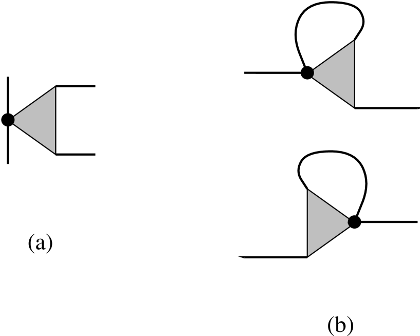
Figure 1: (a) The effective operator, eq.(3.27), in the case of one quark flavor, $N_{f}=1$. (b) Diagrams contributing to the matrix element of the effective operator in quark states.

The effective operator, eq.(3.27), in this case is a four–fermionic operator. It has the form of a color–octet current–current interaction, with one current formed by the fermion fields present in the original QCD operator, the other by the non-local instanton–induced vertices. Graphically it can be represented as in Fig.(1).

In the case of more than one quark flavor, $N_{f}>1$, the effective operator is obtained at first as a $(2N_{f}+2)$–fermionic operator, eq.(3.27). When passing to the bosonized effective theory, eq.(3.11), one may convert also the effective operator to a simple “bosonized” form. Consider a correlation function with the effective many–fermionic operator, eq.(3.27), in the bosonized theory. The correlation function is evaluated by averaging first over the fermion fields in the background of the pion field, later over the pion field (in saddle–point approximation). Let us denote the result of the averaging over the fermions fields by $\langle\ldots\rangle_{\pi}$. In the leading order of $1/N_{c}$ one finds

$$\left\langle\ldots\psi^{\dagger}(x)\Gamma_{\alpha_{1}\ldots\alpha_{r}}\frac{\lambda^{a}}{2}\psi(x)\left[(Y_{+{\cal F}})^{a}_{\beta_{1}\ldots\beta_{s}}(x)+(Y_{-{\cal F}})^{a}_{\beta_{1}\ldots\beta_{s}}(x)\right]\ldots\right\rangle_{\pi}$$ (3.31)

$$= \frac{(iM)^{N_{f}}}{N_{c}}\sum_{f,g=1}^{N_{f}}\int d^{4}z\,{\cal F}_{+,\mu\nu\beta_{1}\ldots\beta_{s}}(x-z)\left\langle\ldots\psi^{\dagger}(x)\Gamma_{\alpha_{1}\ldots\alpha_{r}}\frac{\lambda^{a}}{2}\psi(x)\;J^{a}_{\pm\mu\nu}(z)_{fg}\ldots\right\rangle_{\pi}$$

$$\times\left(\frac{2V}{N}\right)^{N_{f}-1}\left\langle{\textstyle{\det^{\prime}_{fg}}}J_{+}(z)\right\rangle_{\pi}$$

$$+ (+\rightarrow-),$$

since the currents $J_{\pm}$ appearing in the subdeterminant are color–singlet. (We remind that the $J_{\pm}$, eq.(3.8), are matrices in flavor indices.) The ellipses here stand for other functions of the fermion fields, e.g. hadronic currents. Computing the last factor in eq.(3.31) explicitly one finds in leading order in $M\bar{\rho}$:

$$\left(i\frac{2V}{N}\right)^{N_{f}-1}\left\langle{\textstyle{\det^{\prime}_{fg}}}J_{\pm}(z)\right\rangle_{\pi} = \left(i\frac{2V}{N}\right)^{N_{f}-1}{\textstyle{\det^{\prime}_{fg}}}\left\langle J_{\pm}(z)\right\rangle_{\pi}\;\;=\;\;U_{\pm}(z)_{fg},$$ (3.32)

where $U_{\pm}(z)$ is the pion field, eq.(3.12). The first equality holds in leading order of $1/N_{c}$, and in the last step we have used the self–consistency condition defining the saddle point of the effective chiral theory. Thus, in the bosonized effective theory, eq.(3.11), the instanton–induced $2N_{f}$–fermionic vertex, eq.(3.20) is equivalent to the 2–fermionic “bosonized” vertex

$$(Y_{{\cal F}\pm})^{a}_{\beta_{1}\ldots\beta_{r}}[\psi^{\dagger},\psi;\pi]_{\rm bosonized} = \frac{iM}{N_{c}}\int d^{4}z\,{\cal F}_{\pm,\mu\nu\beta_{1}\ldots\beta_{s}}(x-z)\sum_{f,g}^{N_{f}}J^{a}_{\pm\mu\nu}(z)_{fg}U_{\pm}(z)_{fg},$$

which is manifestly chirally invariant. This expression formally includes the case $N_{f}=1$, eq.(3.28), if the pion field is set to zero, $U_{\pm}=1$. Accordingly, the effective operator representing the gluonic operator, eq.(3.17), is again equivalent to a 4–fermionic operator,

$$\mbox{``$O$''}_{\alpha_{1}\ldots\alpha_{r}\beta_{1}\ldots\beta_{s}}[\psi^{\dagger},\psi;\pi](x)$$ (3.34)

$$= -i\psi^{\dagger}(x)\frac{\lambda^{a}}{2}\Gamma_{\alpha_{1}\ldots\alpha_{r}}\psi(x)\left[(Y_{{\cal F}+})^{a}_{\beta_{1}\ldots\beta_{s}}(x)_{\rm bosonized}+(Y_{{\cal F}-})^{a}_{\beta_{1}\ldots\beta_{s}}(x)_{\rm bosonized}\right],$$

which now, however, is coupled to the pion field. This representation of the effective operator is useful for calculations of nucleon matrix elements, see Section 4. It is also of principal interest, since it makes manifest the chiral invariance of the effective operator.

3.3 Matrix elements of higher–twist operators in quark states

Before computing the nucleon matrix elements of higher–twist operators it is instructive to analyze their matrix elements in “constituent quark” states, i.e., the massive quark states corresponding to the fermion fields of the effective chiral theory, eq.(3.6). A pole appears in the quark propagator after continuation to Minkowskian momenta, that is, at Euclidean $p^{2}=-M^{2}+O(M\bar{\rho})$.

Let us first compute the quark matrix element of the effective operator corresponding to the general gluonic operator, eq.(3.17). It is sufficient to consider one quark flavor, $N_{f}=1$, in which case the effective operator is given by the 4–fermionic operator, eq.(3.27), with the instanton–induced vertices eq.(3.28). It is convenient to carry out the entire calculation using Euclidean fields and Euclidean vector components, and to continue to $p^{2}=-M^{2}$ at the end. The quark propagator in the effective theory is given by

$$G(k) = \frac{k/\hskip 1.49994pt+iMF^{2}(k)}{k^{2}+M^{2}F^{4}(k)}.$$ (3.35)

When computing the matrix elements of the 4–fermionic operator between quark states there are two contractions (see Fig.1). One obtains

$$\langle pS|\mbox{``$O$''}_{\alpha_{1}\ldots\alpha_{r}\beta_{1}\ldots\beta_{s}}|pS\rangle\;\;=\;\;\frac{iM}{2}\int\!\frac{d^{4}k}{(2\pi)^{4}}{\cal F}_{+,\mu\nu\beta_{1}\ldots\beta_{s}}(k)$$ (3.36)

$$\times \left\{\frac{F(p)F(p-k)}{(p-k)^{2}+M^{2}F^{4}(p-k)}\;{\rm tr}\,\left[\Lambda_{p,S}\,\Gamma_{\alpha_{1}\ldots\alpha_{r}}\left(p/\hskip 1.49994pt-k/\hskip 1.49994pt+iMF^{2}(p-k)\right)\sigma_{\mu\nu}\frac{1+\gamma_{5}}{2}\right]\right.$$

$$+\left.\frac{F(p)F(p+k)}{(p+k)^{2}+M^{2}F^{4}(p+k)}\;{\rm tr}\,\left[\Lambda_{p,S}\,\sigma_{\mu\nu}\frac{1+\gamma_{5}}{2}\left(p/\hskip 1.49994pt+k/\hskip 1.49994pt+iMF^{2}(p+k)\right)\Gamma_{\alpha_{1}\ldots\alpha_{r}}\right]\right\}$$

$$+ \left({\cal F}_{+,\mu\nu\beta_{1}\ldots\beta_{s}}\rightarrow{\cal F}_{-,\mu\nu\beta_{1}\ldots\beta_{s}},\;\;\frac{1+\gamma_{5}}{2}\rightarrow\frac{1-\gamma_{5}}{2}\right).$$

It is understood that one sets $p^{2}=-M^{2}$ after evaluating the integrals. Here

$$\Lambda_{p,S} = u(p,S)\bar{u}(p,S)\;\;=\;\;\frac{-ip/\hskip 1.49994pt+M}{2}\left(1+i\gamma_{5}S/\hskip 3.00003pt\right)$$ (3.37)

is the projector on quark states with definite momentum and polarization vector, where $p$ and $S$ are Euclidean 4–vectors satisfying

$$p^{2} = -M^{2},\hskip 20.00003ptS^{2}\;=\;1,\hskip 20.00003ptS\cdot p\;=\;0.$$ (3.38)

A factor of $N_{c}$ resulting from the quark loop has canceled the factor $1/N_{c}$ in the effective operator, eq.(3.28), so that the result is $O(N_{c}^{0})$. Eq.(3.36) is understood as the diagonal matrix element for a quark state of given color. We remind that formula eq.(3.36) is valid for operators with zero vacuum expectation value, see the discussion in Section 3.2.

We now apply the general formula eq.(3.36) to the spin–dependent quark matrix elements of the twist–3 and 4 operators, eqs.(2.10, 2.7). In the case of $f^{(2)}$ we simply contract eq.(2.10) with the polarization vector, $S$; to calculate $d^{(2)}$ we contract eq.(2.7) with a light–like vector, $n$, which we choose orthogonal to the polarization vector in order to put the trace terms in eq.(2.7) to zero,

$$n^{2}\;=\;0,\hskip 56.9055ptn\cdot S\;=\;0.$$ (3.39)

Passing to Euclidean fields and vector components we have

$$2M^{3}f^{(2)}_{\rm quark} = -S_{\beta}\;\langle pS|\bar{\psi}\gamma_{\alpha}\widetilde{F}_{\beta\alpha}\psi|pS\rangle,$$ (3.40)

$$4M^{3}d^{(2)}_{\rm quark} = n_{\alpha}n_{\beta}S_{\gamma}\;\langle pS|\bar{\psi}\gamma_{\alpha}\widetilde{F}_{\beta\gamma}\psi|pS\rangle.$$ (3.41)

To evaluate this matrix element we need the Fourier transform of the dual of the field strength of one $I$ and $\bar{I}$, eq.(3.14), which is given by

$$\pm\int d^{4}x\,\exp(-ik\cdot x)\frac{8\rho^{2}}{(x^{2}+\rho^{2})^{2}}\left(\frac{x_{\mu}x_{\beta}}{x^{2}}\delta_{\gamma\nu}+\frac{x_{\nu}x_{\gamma}}{x^{2}}\delta_{\mu\beta}-{\textstyle{\frac{1}{2}}}\delta_{\mu\beta}\delta_{\gamma\nu}\right)$$ (3.42)

$$= \pm\rho^{2}{\cal G}(k)\left(\frac{k_{\mu}k_{\beta}}{k^{2}}\delta_{\gamma\nu}+\frac{k_{\nu}k_{\gamma}}{k^{2}}\delta_{\mu\beta}-{\textstyle{\frac{1}{2}}}\delta_{\mu\beta}\delta_{\gamma\nu}\right),$$

$${\cal G}(k) = 32\pi^{2}\left[\left(\frac{1}{2}+\frac{4}{t^{2}}\right)K_{0}(t)+\left(\frac{2}{t}+\frac{8}{t^{3}}\right)K_{1}(t)-\frac{8}{t^{4}}\right],\hskip 28.45274ptt\;=\;k\rho,$$ (3.43)

where $K_{n}(t)$ are modified Bessel functions of the second kind. Inserting this in eq.(3.36), adding the contributions from $I$’s and $\bar{I}$’s, we obtain

$$2M^{3}f^{(2)}_{\rm quark} = 3M\bar{\rho}^{-2}\;I_{1}(p),$$

$$I_{1}(p) = \bar{\rho}^{4}\int\!\frac{d^{4}k}{(2\pi)^{4}}\frac{{\cal G}(k)F(p)F(p-k)}{(p-k)^{2}+M^{2}F^{4}(p-k)}\,k\cdot p,$$ (3.44)

and

$$4M^{3}d^{(2)}_{\rm quark} = -2M^{3}\;I_{2}(p),$$

$$I_{2}(p) = \bar{\rho}^{-2}\int\!\frac{d^{4}k}{(2\pi)^{4}}\frac{{\cal G}(k)F(p)F^{3}(p-k)}{(p-k)^{2}+M^{2}F^{4}(p-k)}\frac{1}{3}\left(-1+4\frac{(k\cdot p)^{2}}{k^{2}p^{2}}\right),$$ (3.45)

where one should set $p^{2}=-M^{2}$ after evaluating the integrals. One observes that $f^{(2)}_{\rm quark}$ and $d^{(2)}_{\rm quark}$ are of different order in the parameter $M\bar{\rho}$. For small $p$ both integrals $I_{1}(p)$ and $I_{2}(p)$ are proportional to $\bar{\rho}^{2}p^{2}$, and thus

$$f^{(2)}_{\rm quark} \sim (M\bar{\rho})^{0},$$

$$d^{(2)}_{\rm quark} \sim (M\bar{\rho})^{2}\log M\bar{\rho}$$ (3.46)

for $M\bar{\rho}\rightarrow 0$. Numerically one finds, evaluating the integrals for small $p$,

$$I_{1}(p) = -\frac{2}{5}\;\bar{\rho}^{2}p^{2},$$

$$f^{(2)}_{\rm quark} = \frac{3}{5}\;\;=\;\;0.6$$ (3.47)

in the limit $M\bar{\rho}\rightarrow 0$, and

$$I_{2}(p) = -0.066\;\bar{\rho}^{2}p^{2},$$

$$d^{(2)}_{\rm quark} = -0.011$$ (3.48)

at the phenomenological value $M\bar{\rho}=0.58$. The different parametric order of the twist–4 and twist–3 matrix elements reflects itself in the numerical values: $d^{(2)}_{\rm quark}$ is more than an order of magnitude smaller than $f^{(2)}_{\rm quark}$.

Similarly, we can apply the general formula eq.(3.36) to the case of the spin–independent twist–4 operator contributing to power corrections to the Gross–Llewellyn-Smith sum rule, eq.(2.13). Contracting eq.(2.13) with the 4–momentum vector and passing to Euclidean fields and vector components we have

$$2M^{4}c^{(2)}_{\rm quark} = p_{\beta}\;{\textstyle{\frac{1}{2}}}\sum_{\rm spin}\langle p|\bar{\psi}\gamma_{\alpha}\gamma_{5}\widetilde{F}_{\beta\alpha}\psi|p\rangle.$$ (3.49)

Evaluating the matrix element with the help of eq.(3.36) and summing over spins we obtain

$$2M^{4}c^{(2)}_{\rm quark} = -3M^{2}\;I_{1}(p).$$ (3.50)

Thus,

$$c^{(2)}_{\rm quark} \sim (M\bar{\rho})^{0},$$ (3.51)

just as the spin–dependent twist–4 matrix element, $f^{(2)}_{\rm quark}$, eq.(3.46), and numerically in the limit $M\bar{\rho}\rightarrow 0$

$$c^{(2)}_{\rm quark} = -\frac{3}{5}\;\;=\;\;-0.6.$$ (3.52)

Finally, we note that an analogous calculation of the forward matrix elements of the operators

$$\langle p|\bar{\psi}\gamma_{\alpha}F_{\beta\alpha}\psi|p\rangle,\hskip 20.00003pt\langle pS|\bar{\psi}\gamma_{\alpha}\gamma_{5}F_{\beta\alpha}\psi|pS\rangle,$$ (3.53)

gives identically zero, as it should be on grounds of the QCD equations of motion. From this we conclude that the method of effective operators preserves a principal feature of QCD: matrix elements of operators which are zero in QCD due to the QCD equations of motion are automatically zero in the effective theory. This remarkable property of effective operators will be investigated in more detail in Section 3.4.

The results obtained here for the quark matrix elements of higher–twist operators can be rephrased in terms of local operators, whose matrix elements reproduce those of the non-local effective 4–fermionic operators at quark level. At momenta of order $M\ll\bar{\rho}^{-1}$ this “localization” is justified by the fact that the effects of the non-locality of the instanton–induced vertices contribute only in higher orders of $M\bar{\rho}$. Since the quark loop integrals in eqs.(3.44, 3.45, 3.50) are proportional to the external momentum $p^{2}$, the local operator which should be valid for general quark momenta $p$ of order $M$, not necessarily on the mass shell $p^{2}=-M^{2}$, must contain derivatives. The twist–4 operator, eq.(2.10), we can thus represent as (in the Euclidean theory)

$$\bar{\psi}\gamma_{\alpha}\widetilde{F}_{\beta\alpha}\psi \rightarrow f^{(2)}_{\rm quark}\;\bar{\psi}\gamma_{\beta}\gamma_{5}\partial^{2}\psi.$$ (3.54)

Up to the derivative the equivalent local operator is the axial current operator, multiplied by the coefficient $f^{(2)}_{\rm quark}$. For the twist–3 operator, eq.(2.7), the corresponding local operator is

$$\bar{\psi}\left(\gamma_{\alpha}\widetilde{F}_{\beta\gamma}+\gamma_{\beta}\widetilde{F}_{\alpha\gamma}\right)\psi \rightarrow -d^{(2)}_{\rm quark}\;\bar{\psi}\left(\partial_{\alpha}\partial_{\left[\beta\right.}\gamma_{\left.\gamma\right]}+\partial_{\beta}\partial_{\left[\alpha\right.}\gamma_{\left.\gamma\right]}\right)\gamma_{5}\psi.$$ (3.55)

For the spin–independent twist–4 operator, eq.(2.13), finally, the equivalent local operator is related to the vector current,

$$\bar{\psi}\gamma_{\alpha}\gamma_{5}\widetilde{F}_{\beta\alpha}\psi \rightarrow c^{(2)}_{\rm quark}\;\bar{\psi}\gamma_{\beta}\partial^{2}\psi.$$ (3.56)

When going to nucleon, for various reasons, a strictly local representation of the higher–twist operators is no longer possible. In the nucleon one finds “sea” quarks with momenta of order of the cutoff, $\bar{\rho}^{-1}$, so one must take into account the full momentum dependence of the instanton–induced vertices. Furthermore, there are interaction contributions to the matrix element in which more than one quark connects to the many–fermionic operator. The local operators are nevertheless useful as a replacement for the non-local effective operator for “valence” quarks whose momenta are restricted to values $\ll\bar{\rho}^{-1}$ by the bound–state wave function of the nucleon. Also, the parametric order in $M\bar{\rho}$ which is encoded in the constants $f^{(2)}_{\rm quark},d^{(2)}_{\rm quark}$ and $c^{(2)}_{\rm quark}$ will carry over to the nucleon matrix elements. In Section 4.4 we shall see to which extent the relation between $f^{(2)}$ and the axial vector coupling constant, $g_{A}$, as well as between $c^{(2)}$ and the vector coupling constant, which holds for on-shell quark matrix elements, is valid also for the nucleon.

3.4 The QCD equation of motion

The set of local operators which are used in the operator product expansion at higher–twist level is overcomplete. Some higher–twist operators can be reduced to other operators, others are identically zero, by the QCD equations of motion. For instance, the twist–4 operator

$$\bar{\psi}(x)\nabla/\hskip 3.00003pt\psi(x) = \bar{\psi}(x)\gamma_{\alpha}\left(\partial_{\alpha}-i\frac{\lambda^{a}}{2}A_{\alpha}^{a}(x)\right)\psi(x)$$ (3.57)

should have zero matrix element in physical states,

$$\langle P|\psi^{\dagger}\nabla/\hskip 3.00003pt\psi|P\rangle = 0.$$ (3.58)

Furthermore, using the fact that in QCD

$$\frac{\lambda^{a}}{2}F_{\beta\alpha}^{a}(x) = i[\nabla_{\beta},\nabla_{\alpha}],$$ (3.59)

one may show that

$$\langle P|\bar{\psi}\gamma_{\alpha}F_{\beta\alpha}\psi|P\rangle = 0.$$ (3.60)

When passing from QCD to the effective theory it is important that these general properties are preserved by the corresponding effective operators. We already noted in Section 3.3 that the matrix element eq.(3.60) in quark states is identically zero. We now want to show in a more general context that eq.(3.58) holds in the effective theory, when the gauge field in the QCD operator, eq.(3.57), is replaced by the corresponding effective operator.

Consider the gauge field part of the QCD operator eq.(3.57). Since we are interested in the forward matrix element we may integrate the operator over the 4–volume,

$$O_{A} = \int d^{4}x\left[\bar{\psi}(x)\gamma_{\alpha}\frac{\lambda^{a}}{2}\psi(x)A_{\alpha}^{a}(x)\right].$$ (3.61)

The effective operator corresponding to this operator is given by eq.(3.23)

“$$O_{A} = \int d^{4}x\left[-i\psi^{\dagger}(x)\gamma_{\alpha}\frac{\lambda^{a}}{2}\psi(x)\left\{(Y_{A+})^{a}_{\alpha}(x)N_{+}{\cal R}_{+}+(Y_{A-})^{a}_{\alpha}(x)N_{-}{\cal R}_{-}\right\}\right].$$” (3.62)

Here the vertices $(Y_{A\pm})^{a}_{\alpha}$ are given by the general formula eq.(3.20), in which one substitutes the gauge potential of one $I$ ($\bar{I}$), eq.(3.15), the Fourier transform of which is given by

$$\int d^{4}x\,e^{-ik\cdot x}\frac{2\rho^{2}}{(x^{2}+\rho^{2})x^{2}}x_{\nu}\delta_{\mu\beta} = -i\rho^{4}{\cal H}(k)k_{\nu}\delta_{\mu\beta},$$ (3.63)

$${\cal H}(k) = \frac{8\pi^{2}}{t^{2}}\left[-\frac{1}{2}K_{0}(t)-\frac{2}{t}K_{1}(t)+\frac{2}{t^{2}}\right],\hskip 28.45274ptt\;=\;k\rho.$$ (3.64)

Consider a correlation function (connected average) of the effective operator eq.(3.62) with external fermion fields. The connected average consists of two parts, in which the external fermion fields connect either to the $2N_{f}$–fermionic vertices, $(Y_{A\pm})^{a}_{\alpha}$, or to the factors ${\cal R}_{\pm}$:

$$\left\langle\psi(y^{\prime})\;\mbox{``$O_{A}$''}\;\psi^{\dagger}(y)\right\rangle_{\rm conn}$$ (3.65)

$$= \left\langle\psi(y^{\prime})\int d^{4}x\left[-i\psi^{\dagger}(x)\gamma_{\mu}\frac{\lambda^{a}}{2}\psi(x)(Y_{A+})^{a}_{\mu}(x)\right]\psi^{\dagger}(y)\right\rangle_{\rm conn}N_{+}\left\langle{\cal R}_{+}\right\rangle$$

$$+ \left\langle\int d^{4}x\left[-i\psi^{\dagger}(x)\gamma_{\mu}\frac{\lambda^{a}}{2}\psi(x)(Y_{A+})^{a}_{\mu}(x)\right]\right\rangle N_{+}\left\langle\psi(y^{\prime}){\cal R}_{+}\psi^{\dagger}(y)\right\rangle_{\rm conn}$$

$$+ (+\rightarrow-).$$

By explicit calculation, using eqs.(3.28, 3.64) and the fact that the form factor $F(k)$ is proportional to the Fourier transform of the instanton zero mode, which implies the relation

$$\int\!\frac{d^{4}k}{(2\pi)^{4}}\;{\cal H}(p-k)\;\frac{(p-k)\cdot k}{k^{2}}\;F(k) = \frac{2i}{3}F(p),$$ (3.66)

one shows that up to terms of order $(M\bar{\rho})^{2}$ the insertion of the $(2N_{f}+2)$–fermionic vertex into the correlation function of fermion fields is equivalent to an insertion of a ’t Hooft vertex, eq.(3.7):

$$\left\langle\psi(y^{\prime})\int d^{4}x\left[-i\psi^{\dagger}(x)\gamma_{\mu}\frac{\lambda^{a}}{2}\psi(x)\;(Y_{A\pm})^{a}_{\mu}(x)\right]\psi^{\dagger}(y)\right\rangle_{\rm conn} = 2\left\langle\psi(y^{\prime})\;Y_{\pm}\;\psi^{\dagger}(y).\right\rangle_{\rm conn}$$

The factor of $2$ appears because, due to the color structure, there are $2N_{f}$ different ways to contract the $(2N_{f}+2)$–fermionic operator on the right–hand side with the external quark fields, but only $N_{f}$ for the $2N_{f}$–fermionic vertices $Y_{\pm}$. On the other hand, the vacuum expectation value of the $(2N_{f}+2)$–fermionic vertex appearing in the second term of eq.(3.65) is

$$\left\langle\int d^{4}x\left[-i\psi^{\dagger}(x)\gamma_{\mu}\frac{\lambda^{a}}{2}\psi(x)\;(Y_{A\pm})^{a}_{\mu}(x)\right]\right\rangle = \left\langle Y_{\pm}\right\rangle\;\;=\;\;N_{\pm}$$ (3.68)

by virtue of the self–consistency condition defining the saddle point. The connected average of the factors ${\cal R}_{\pm}$ with external fermion fields is given by eq.(3.26), which is a consequence of their definition as the “inverse” of the ’t Hooft vertices. Putting these results together, one observes that the sum of the two terms of eq.(3.65) combines to give

$$\left\langle\psi(y^{\prime})\;\mbox{``$O_{A}$''}\;\psi^{\dagger}(y)\right\rangle_{\rm conn} = \left\langle\psi(y^{\prime})\;Y_{\pm}\;\psi^{\dagger}(y)\right\rangle_{\rm conn}.$$ (3.69)

We have thus shown that, to order $(M\bar{\rho})^{2}$, the gluonic part of the QCD equations of motion, eq.(3.58), corresponds to an insertion of the ’t Hooft vertex in the effective theory. The operator corresponding to the QCD equations of motion thus vanishes by virtue of the equations of motion of the effective theory, a very gratifying result. This serves as additional confirmation that the approximations made in deriving the effective action and the effective operators are mutually consistent.

3.5 Non-leading vs. leading twist

In section 3.3 it was shown that matrix elements of gluonic operators of twist 4 are of order unity in the packing fraction of the instanton medium, while those of twist 3 are suppressed. We now want to investigate the role of instantons in operators of twist 2, which determine the scaling (non–power suppressed) part of nucleon structure functions. In particular, using the method of effective operators, we want to see why — and under which conditions — it is justified to drop the gluon field in twist–2 QCD operators when passing to the effective chiral theory. This approximation of “quarks–antiquarks only” is used in all calculations of leading–twist structure functions of the nucleon in the effective chiral theory [15, 16].

Consider the twist–2 QCD operator of spin $n+1$, eq.(2), which determines the $n$’th moment of the polarized structure function, $g_{1}$ (for simplicity let us consider one flavor, $N_{f}=1$). With the explicit form of the covariant derivative,

$$\nabla_{\mu} = \partial_{\mu}-i\frac{\lambda^{a}}{2}A_{\mu}^{a}(x),$$ (3.70)

the operator can be written as a part containing only explicit derivatives, plus terms involving powers of the gauge field,

$$\bar{\psi}\gamma_{\left\{\alpha\right.}\gamma_{5}\nabla_{\beta_{1}}\ldots\nabla_{\left.\beta_{n}\right\}}\psi = \bar{\psi}\gamma_{\left\{\alpha\right.}\gamma_{5}\partial_{\beta_{1}}\ldots\partial_{\left.\beta_{n}\right\}}\psi$$ (3.71)

$$- i\sum_{i}^{n}\bar{\psi}\gamma_{\left\{\alpha\right.}\gamma_{5}\partial_{\beta_{1}}\ldots A^{a}_{\beta_{i}}\ldots\partial_{\left.\beta_{n}\right\}}\frac{\lambda^{a}}{2}\psi$$

$$+ \mbox{terms}\;\;A^{2},A^{3}\ldots$$

When passing to the effective chiral theory, the pure derivative part becomes simply the corresponding operator in terms of fields of the effective theory, while the terms involving the gauge field have to be replaced by the corresponding effective operators; they are of the form of the general operator eq.(3.17). Let us consider the matrix elements of eq.(3.71) in quark states of the effective theory. The matrix element of the pure derivative part is trivial and contributes precisely unity to the moment $a^{(n)}$. On the other hand, using the general formulas of sections 3.2 and 3.3 one easily shows that the matrix element of the terms involving the gauge field is of order $(M\bar{\rho})^{2}$. Thus,

$$a^{(n)}_{\rm quark} = 1\;+\;O\left((M\bar{\rho})^{2}\right).$$ (3.72)

The contribution of the gauge field is parametrically suppressed relative to the pure derivatives. In terms of the structure function $g_{1}$ this implies

$$g_{1}(x)_{\rm quark} = {\textstyle{\frac{1}{2}}}\delta(x-1)\;+\;O\left((M\bar{\rho})^{2}\right).$$ (3.73)

To leading order in $M\bar{\rho}$ the quark of the effective chiral theory is “elementary”, it structure in the instanton vacuum emerges only at level $(M\bar{\rho})^{2}$.

At the same time, one finds that the twist–2 QCD operators determining the moments of the polarized gluon distribution,

$$\langle PS|F_{\left\{\alpha\beta\right.}D_{\beta_{1}}\ldots D_{\beta_{n-1}}\widetilde{F}^{\beta}_{\left.\beta_{n}\right\}}|PS\rangle-\mbox{traces}$$ (3.74)

$$= 2M_{N}\;b^{(n)}\;S_{\left\{\alpha\right.}P_{\beta_{1}}\ldots P_{\left.\beta_{n}\right\}}-\mbox{traces},$$

are identically zero when one substitutes the field of one instanton (the same applies to the unpolarized gluon distribution.) The reason is the $O(4)$ symmetry of the instanton field: after integration over instanton coordinates one can build the $\beta_{1}\ldots\beta_{n}$ tensor only out of Kronecker symbols, so it is impossible to get it traceless. Thus the effective operator for eq.(3.74) is zero. However, the operator in eq.(3.74) becomes non-zero when taking into account two–instanton contributions, which are parametrically suppressed by a factor $(\bar{\rho}/R)^{4}\propto(M\bar{\rho})^{2}$. We conclude that

$$b^{(n)} = O\left((M\bar{\rho})^{2}\right).$$ (3.75)

To summarize, we see that in twist–2 operators the effect of the instanton field is always of order $(M\bar{\rho})^{2}$. When working to leading order in $M\bar{\rho}$, it is consistent to keep only the pure derivative part in the twist–2 quark operators, eq.(3.71), and to replace the operators for the twist–2 gluon distribution by zero. This is the approximation employed in the calculation of the twist–2 part of the nucleon structure functions in refs.[15, 16, 17].

However, as we have seen above, instantons can make contributions of order unity in higher–twist operators. In the cases considered in section 3.3 the first non-suppressed instanton contributions appeared at twist 4. There can of course also be $O((M\bar{\rho})^{2})$ contributions to operators of twist 6 and higher.

The difference between the instanton contribution to operators of leading and non-leading twist can be seen even more clearly in the case of unpolarized structure functions. The second moment of the structure function $F_{2}$, $M^{(2)}$, is given by the matrix element of the twist–2 spin–2 operator,

$$\langle P|\bar{\psi}\gamma_{\left\{\mu_{1}\right.}\nabla_{\left.\mu_{2}\right\}}\psi|P\rangle-\mbox{traces} = M^{(2)}P_{\left\{\mu_{1}\right.}P_{\left.\mu_{2}\right\}}-\mbox{traces}.$$ (3.76)

In analogy to eq.(3.72), at quark level the pure derivative term makes unity contribution to $M^{(2)}$, while the contribution of the gauge field is suppressed by $(M\bar{\rho})^{2}$:

$$M^{(2)}_{\rm quark} = 1\;+\;O\left((M\bar{\rho})^{2}\right)$$ (3.77)

This is consistent with the energy–momentum sum rule, since the momentum carried by gluons is $O((M\bar{\rho})^{2})$, cf. eq.(3.75). On the other hand, if one does not project on twist 2 but contracts the indices in eq.(3.76) one obtains the twist–4 matrix element

$$\langle P|\bar{\psi}\nabla/\hskip 3.00003pt\psi|P\rangle = CM^{2},$$ (3.78)

where $C=0$ by virtue of the equations of motion. As was is shown in section 3.4, this zero comes because an order unity contribution to $C$ from the instanton field exactly cancels the pure derivative term in the Dirac operator.

4 Nucleon matrix elements of higher–twist operators

4.1 The nucleon in the effective chiral theory

An immediate application of the effective chiral theory derived from the instanton vacuum is the chiral quark soliton model of the nucleon [13]. In this section we briefly recall the main characteristics of this description.

In the effective chiral theory the nucleon is described in the large–$N_{c}$ limit by a classical pion field, $U_{c}({\bf x})$. The quarks single-particle wave functions are determined from the Dirac equation in the external pion field,

$$H\Phi_{n}({\bf x}) = E_{n}\Phi_{n}({\bf x}),$$ (4.1)

$$H = \gamma_{4}\left[\gamma_{k}\partial_{k}-MU^{\gamma_{5}}({\bf x})\right],$$ (4.2)

$$U^{\gamma_{5}} = \exp\left[i\pi^{a}(x)\tau^{a}\gamma_{5}\right]\;\;=\;\;\frac{1+\gamma_{5}}{2}U_{+}(x)+\frac{1-\gamma_{5}}{2}U^{\dagger}(x).$$ (4.3)

The spectrum of the one-particle Hamiltonian, $H$, contains the upper and lower Dirac continua (distorted by the presence of the external pion field), as well as a discrete bound–state level. We denote the energy of this discrete level by $E_{\rm lev},\;\;-M\leq E_{\rm lev}\leq M$. This level must be occupied by $N_{c}$ quarks to have a state of unit baryon number. The saddle point pion field is determined by minimizing the static energy, which includes the energy of the discrete level as well as the aggregate energy of the negative Dirac continuum. It is of “hedgehog” form,

$$U_{c}({\bf x})\;=\;\exp\left[i\pi^{a}({\bf x})\tau^{a}\right]\;=\;\exp\left[\frac{i{\bf x}\cdot\mbox{\boldmath{$\tau$}}}{r}P(r)\right],\hskip 28.45274ptr\;=\;|{\bf x}|,$$ (4.4)

where $P(r)$ is called the profile function. A variational approximation to the soliton profile in the form

$$P(r) = 2\;\arctan\left(\frac{r_{0}^{2}}{r^{2}}\right)$$ (4.5)

with $r_{0}\approx 1.0/M$ gives a very reasonable description of a variety of static nucleon observables [13].

The minimum of the energy is degenerate with respect to translations of the soliton in space and to rotations of the soliton field in ordinary and isospin space. For the hedgehog field eq.(4.4) the two rotations are equivalent. Quantizing slow rotations of the saddle-point pion field gives rise to the quantum numbers of the nucleon: its spin and isospin components [28, 13]. In order to take into account the translational and rotational zero modes one has to perform a rotation of the soliton field in flavor space and to shift its center,

$$U({\bf x}) = RU_{c}({\bf x}-{\bf X})R^{\dagger},$$ (4.6)

the same for the quark eigenfunctions,

$$\Phi_{n}({\bf x}) \rightarrow R\Phi_{n}({\bf x}-{\bf X}),$$ (4.7)

and to make a projection to a concrete nucleon state under consideration. The projection on a nucleon state with given momentum ${\bf P}$ is obtained by integrating over all shifts ${\bf X}$ of the soliton,

$$\langle{\bf P^{\prime}}|\ldots|\ {\bf P}\rangle = \int d^{3}{\bf X}\;e^{i({\bf P^{\prime}-P})\cdot{\bf X}}\;\ldots.$$ (4.8)

The projection on a nucleon with given spin ($S_{3}$) and isospin ($T_{3}$) components is obtained by integrating over all spin-isospin rotations $R$ of the soliton,

$$\langle S=T,S_{3},T_{3}|\ldots|S=T,S_{3},T_{3}\rangle = \int dR\;\phi^{\dagger\;S=T}_{S_{3}T_{3}}(R)\;\ldots\;\phi^{S=T}_{S_{3}T_{3}}(R),$$ (4.9)

where $\phi^{S=T}_{S_{3}T_{3}}(R)$ is the rotational wave function of the nucleon given by the Wigner finite-rotation matrix [13]:

$$\phi^{S=T}_{S_{3}T_{3}}(R) = \sqrt{2S+1}(-1)^{T+T_{3}}D^{S=T}_{-T_{3},S_{3}}(R).$$ (4.10)

The four nucleon states have $S=T=1/2$, with $S_{3},T_{3}=\pm 1/2$. It is implied that $dR$ in eq.(4.9) is the Haar measure normalized to unity. (In the following we shall omit the superscript $S=T$.)

4.2 Nucleon matrix elements of effective gluon operators

We now turn to the calculation of nucleon matrix elements of the effective operators which arise in the description of higher–twist corrections. In this subsection we derive the expressions for the nucleon matrix element of the general gluonic operator, eq.(3.17), which was considered in Sections 3.2 and 3.3,

$$O_{\alpha_{1}\ldots\alpha_{r}\beta_{1}\ldots\beta_{s}}(x) = \bar{\psi}(x)\;\hat{t}\;\frac{\lambda^{a}}{2}\Gamma_{\alpha_{1}\ldots\alpha_{r}}\,\psi(x)\;{\cal F}^{a}_{\beta_{1}\ldots\beta_{s}}(x),$$

where we have introduced now a flavor matrix, $\hat{t}$, with $\hat{t}=\tau^{3}$ for the flavor–nonsinglet and $\hat{t}=1$ for the singlet case.

To compute the nucleon matrix element we use the bosonized form of the effective operator, eq.(3.34), where the pion field is to be replaced by the soliton field, eq.(4.4):

$$\mbox{``$O$''}_{\alpha_{1}\ldots\alpha_{r}\beta_{1}\ldots\beta_{s}}(x)$$ (4.11)

$$= \frac{iM}{N_{c}}\int d^{4}z\,{\cal F}_{+,\mu\nu\beta_{1}\ldots\beta_{s}}(x-z)$$

$$\times\left[-i\psi^{\dagger}(x)\;\hat{t}\;\frac{\lambda^{a}}{2}\Gamma_{\alpha_{1}\ldots\alpha_{r}}\psi(x)\right]\;\left[\psi^{\dagger}(z)\frac{\lambda^{a}}{2}\sigma_{\mu\nu}U_{+}({\bf z})\frac{1+\gamma_{5}}{2}\psi(z)\right]$$

$$+ \left({\cal F}_{+,\mu\nu\beta_{1}\ldots\beta_{s}}\rightarrow{\cal F}_{-,\mu\nu\beta_{1}\ldots\beta_{s}},\;\;\frac{1+\gamma_{5}}{2}\rightarrow\frac{1-\gamma_{5}}{2},\;\;U_{+}\rightarrow U_{-}\right).$$

(For simplicity we have neglected for the moment the nonlocality of the instanton–induced vertices, i.e., we have set the form factor $F(k)\equiv 1$. The form factors will be inserted again later.) This operator has the form of a product of two color–octet currents, similar to one–gluon exchange between quarks, with the functions ${\cal F}_{\pm,\mu\nu\beta_{1}\ldots\beta_{s}}$ playing the role of the gluon propagator. The calculation of the nucleon matrix element of the effective operator is thus analogous to that of gluon exchange corrections to the nucleon mass [29]. One expands the quark fields in eq.(3.34) in the basis of single–particle wave functions, eq.(4.1), and computes the matrix element, summing over all occupied quark single–particle levels including the bound–state level and the negative Dirac continuum. In addition, one has to perform a rotation and shift of the center of the pion field and the quark wave functions, eqs.(4.6 , 4.7), and integrate over collective wave functions to project on a nucleon state with given spin–isospin quantum numbers. One obtains

$$\langle{\bf P}=0,T_{3},S_{3}|\mbox{``$O$''}_{\alpha_{1}\ldots\alpha_{r}\beta_{1}\ldots\beta_{s}}|{\bf P}=0,T_{3},S_{3}\rangle$$ (4.12)

$$= 2M_{N}\int dR\,\phi_{S_{3}T_{3}}^{\dagger}(R)\phi_{S_{3}T_{3}}(R)\;{\cal M}_{\alpha_{1}\ldots\alpha_{r}\beta_{1}\ldots\beta_{s}}(R),$$

$${\cal M}_{\alpha_{1}\ldots\alpha_{r}\beta_{1}\ldots\beta_{s}}(R)$$ (4.13)

$$= -\frac{N_{c}}{2T}\int d^{4}x\int d^{4}z\;{\cal F}_{+,\mu\nu\beta_{1}\ldots\beta_{s}}(x-z)\;{\sum_{m,n}}^{\prime}\exp\left[(E_{n}-E_{m})(x_{4}-z_{4})\right]$$

$$\times\left[\Phi_{n}^{\dagger}({\bf x})\gamma_{4}\;R^{\dagger}\hat{t}R\;\Gamma_{\alpha_{1}\ldots\alpha_{r}}\Phi_{m}({\bf x})\right]\left[\Phi_{m}^{\dagger}({\bf z})\gamma_{4}\;\sigma_{\mu\nu}\frac{1+\gamma_{5}}{2}MU_{+}({\bf z})\;\Phi_{n}({\bf z})\right]$$

$$+ (+\rightarrow-),$$

where

$${\sum_{m,n}}^{\prime} = \theta(x_{4}-z_{4})\sum\limits_{\scriptstyle n\atop\scriptstyle{\rm occ.}}\sum\limits_{\scriptstyle m\atop\scriptstyle{\rm non-occ.}}\;+\;\theta(z_{4}-x_{4})\sum\limits_{\scriptstyle n\atop\scriptstyle{\rm non-occ.}}\sum\limits_{\scriptstyle m\atop\scriptstyle{\rm occ.}}.$$ (4.14)

Here we have used that for the forward matrix element, ${\bf P}={\bf P}^{\prime}=0$, the integral over translations is trivial. Due to translational invariance it is equivalent to integrating the coordinate of the operator, $x$, eq.(3.34), over the 3–volume. To obtain a more symmetric form, we have integrated over the Euclidean 4–volume and divided by the Euclidean time interval, $T$. In the following we shall drop the labels ${\bf P}=0$.

A factor of $N_{c}^{2}/2$ resulting from the sum over color indices combines with the factor $1/N_{c}$ in the effective operator eq.(3.34), to give an overall factor of $N_{c}/2$.

To proceed with the evaluation of eq.(4.13) one has to perform the integral over soliton rotations, considering separately flavor singlet and nonsinglet operators. We note that the factor $\Phi^{\dagger}_{m}\ldots U_{\pm}\ldots\Phi_{n}$ in eq.(4.13) does not depend on the rotation matrices, as it should be. This factor represents the “gluonic” part of the operator eq.(4.11), and is thus by definition a flavor singlet.

One easily sees that for spin–dependent matrix elements such as $d^{(2)}$ and $f^{(2)}$, eqs.(2.7, 2.10), the flavor–nonsinglet part appears in the leading order of the $1/N_{c}$–expansion. In this case in eq.(4.13) $\hat{t}=\tau^{3}$, and the integral over rotations is performed using

$$R^{\dagger}\tau^{3}R = D_{3a}(R)\tau^{a},\hskip 20.00003ptD_{ab}(R)\;\;=\;\;{\textstyle{\frac{1}{2}}}\,{\rm tr}\,\left[R^{\dagger}\tau^{a}R\tau^{b}\right],$$ (4.15)

$$\int dR\,\phi_{S_{3}T_{3}}^{\dagger}(R)D_{3a}(R)\phi_{S_{3}T_{3}}(R) = -\frac{1}{3}(\tau^{3})_{T_{3}T_{3}}(\sigma^{a})_{S_{3}S_{3}}.$$ (4.16)

The non-singlet matrix element thus becomes

$$\langle T_{3},S_{3}|\mbox{``$O$''}^{NS}_{\alpha_{1}\ldots\alpha_{r}\beta_{1}\ldots\beta_{s}}|T_{3},S_{3}\rangle_{\rm spin-dep.} = -2M_{N}(2T_{3})\frac{S_{a}}{3}\;{\cal M}^{a}_{\alpha_{1}\ldots\alpha_{r}\beta_{1}\ldots\beta_{s}},$$

$${\cal M}^{a}_{\alpha_{1}\ldots\alpha_{r}\beta_{1}\ldots\beta_{s}} = -\frac{N_{c}}{2T}\int d^{4}x\int d^{4}z{\cal F}_{+,\mu\nu\beta_{1}\ldots\beta_{s}}(x-z){\sum_{m,n}}^{\prime}\exp\left[(E_{n}-E_{m})(x_{4}-z_{4})\right]$$ (4.17)

$$\times\left[\Phi_{n}^{\dagger}({\bf x})\gamma_{4}\tau^{a}\Gamma_{\alpha_{1}\ldots\alpha_{r}}\Phi_{m}({\bf x})\right]\left[\Phi_{m}^{\dagger}({\bf z})\gamma_{4}\sigma_{\mu\nu}\frac{1+\gamma_{5}}{2}MU_{+}({\bf z})\Phi_{n}({\bf z})\right]$$

$$+ (+\rightarrow-).$$

Here $S_{a}\;(a=1,2,3)$ are the components of the nucleon polarization vector in the rest frame,

$$S = (0,{\bf S}),\hskip 20.00003pt{\bf S}\;\;=\;\;(0,0,1).$$ (4.18)

For spin–independent matrix elements such as $c^{(2)}$, eqs.(2.13), on the other hand, the flavor singlet part is leading in $N_{c}$. In the flavor singlet case $\hat{t}=1$, the orientation matrices $R,R^{\dagger}$ are contracted, and the integral over rotations becomes trivial,

$$\int dR\,\phi_{S_{3}T_{3}}^{\dagger}(R)\phi_{S_{3}T_{3}}(R) = 1.$$ (4.19)

One obtains

$$\langle T_{3}S_{3}|\mbox{``$O$''}^{S}_{\alpha_{1}\ldots\alpha_{r}\beta_{1}\ldots\beta_{s}}|T_{3}S_{3}\rangle_{\rm spin-dep.} = 2M_{N}\;{\cal M}_{\alpha_{1}\ldots\alpha_{r}\beta_{1}\ldots\beta_{s}},$$

$${\cal M}_{\alpha_{1}\ldots\alpha_{r}\beta_{1}\ldots\beta_{s}} = (\ref{O_NS_levels})\;\;\;\mbox{with}\;\;\;\tau^{a}\rightarrow 1.$$ (4.20)

The isosinglet spin–dependent and isovector spin–independent matrix elements are zero in the leading order of the $1/N_{c}$–expansion. They appear only after including rotational corrections to eq.(4.13), i.e., integrating over time–dependent rotations and expanding in the angular frequency, which is of order $1/N_{c}$.

The $N_{c}$–ordering of the matrix elements of twist–3 and 4 operators is analogous to the one of the twist–2 quark distribution functions, where the isovector–polarized and isosinglet–unpolarized distributions appear in the leading order of the $1/N_{c}$–expansion. The connection between spin and isospin is a general consequence of the hedgehog symmetry of the pion field, eq.(4.4). For reference, we have listed order of the various matrix elements in $N_{c}$ in table 1.

We have obtained a closed expression for the matrix element of the effective operator corresponding to a general gluonic operator eq.(3.17), in the form of a sum over quark single–particle levels in the pion field of the soliton. This representation is useful for studying the $N_{c}$–order of different spin–isospin combinations. Moreover, eq.(4.13) could serve as a starting point for numerical calculations of the matrix elements, using the quark wave functions determined by numerical diagonalization of the Dirac Hamiltonian, eq.(4.1), in a finite box [14, 16]. For further theoretical analysis, however, it is convenient to pass to the more familiar language of Feynman diagrams. Substituting in eq.(4.13) the spectral representation of the quark Green function in the background pion field,

$$G(x,y) = \theta(x_{4}-y_{4})\sum_{E_{n}>0}\exp\left[-E_{n}(x_{4}-y_{4})\right]\Phi_{n}({\bf x})\Phi_{n}^{\dagger}({\bf y})i\gamma_{4}$$ (4.21)

$$- \theta(y_{4}-x_{4})\sum_{E_{n}<0}\exp\left[-E_{n}(x_{4}-y_{4})\right]\Phi_{n}({\bf x})\Phi_{n}^{\dagger}({\bf y})i\gamma_{4},$$

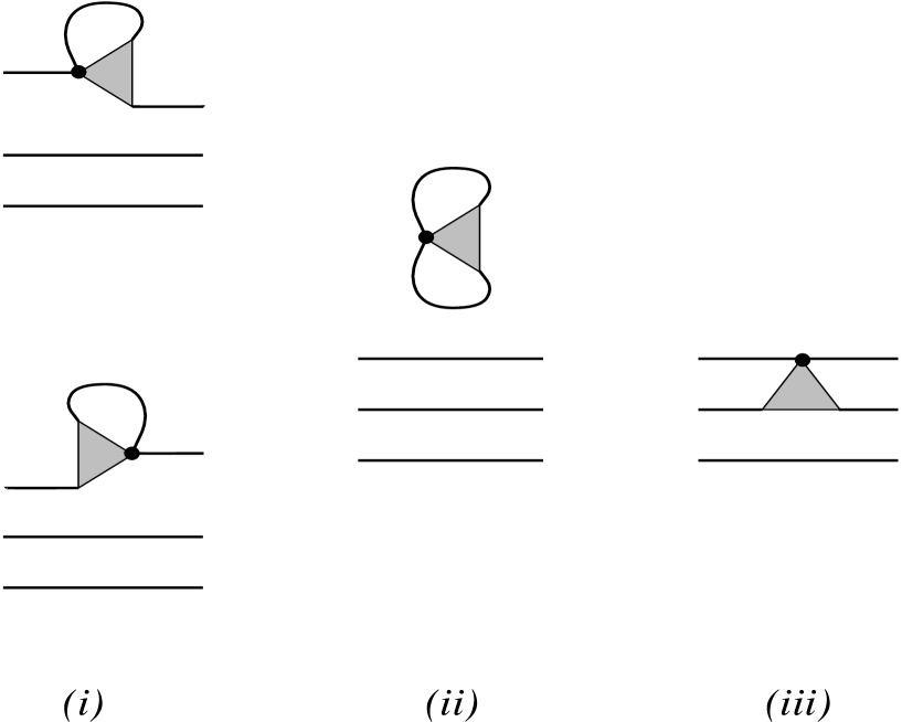
Figure 2: Feynman diagrams contributing to the nucleon matrix element of the effective operator. (i) “Valence quark” contribution, eq.(4.23) (ii) “Sea quark” contribution, eq.(4.24). (iii) Interaction contribution, eq.(4.27).

and rearranging the terms in the sum over quark levels, one can show that eq.(4.13) is equal to the sum of three terms which correspond to the Feynman diagrams for the 3–point correlation function shown in Fig.2,

$$\langle T_{3},S_{3}|\mbox{``$O$''}^{NS}_{\alpha_{1}\ldots\alpha_{r}\beta_{1}\ldots\beta_{s}}|T_{3},S_{3}\rangle_{\rm spin-dep.}$$ (4.22)

$$= -2M_{N}(2T_{3})\frac{S_{a}}{3}\left[{\cal M}_{(i)}^{a}+{\cal M}_{(ii)}^{a}+{\cal M}_{(iii)}^{a}\right]_{\alpha_{1}\ldots\alpha_{r}\beta_{1}\ldots\beta_{s}}.$$

We write them down for the spin–dependent isovector matrix element, eq.(4.17); the corresponding expressions for the spin–independent isoscalar matrix elements are obtained by the trivial substitution eq.(4.20):

(i) A “valence quark” contribution in which the effective operator connects to one valence quark line:

$${\cal M}^{a}_{\alpha_{1}\ldots\alpha_{r}\beta_{1}\ldots\beta_{s},\,(i)}$$ (4.23)

$$= -\frac{N_{c}}{2T}\int d^{4}x\int d^{4}z{\cal F}_{+,\mu\nu\beta_{1}\ldots\beta_{s}}(x-z)$$

$$\times \left\{\exp\left[E_{\rm lev}(x_{4}-z_{4})\right]\Phi_{\rm lev}^{\dagger}({\bf x})\left[\gamma_{4}\Gamma_{\alpha_{1}\ldots\alpha_{r}}\tau^{a}G(x,z)\gamma_{4}\sigma_{\mu\nu}\frac{1+\gamma_{5}}{2}MU_{+}({\bf z})\right]\Phi_{\rm lev}({\bf z})\right.$$

$$+\left.\exp\left[-E_{\rm lev}(x_{4}-z_{4})\right]\Phi_{\rm lev}^{\dagger}({\bf z})\left[\gamma_{4}\sigma_{\mu\nu}\frac{1+\gamma_{5}}{2}MU_{+}({\bf z})\tau^{a}\Gamma_{\alpha_{1}\ldots\alpha_{r}}G(z,x)\gamma_{4}\right]\Phi_{\rm lev}({\bf x})\right\}$$

$$+ (+\rightarrow-).$$

This contribution has the form of a quark self-energy diagram evaluated between bound–state wave functions. This contribution is similar to the Lamb shift in atomic physics.

(ii) A “sea quark” contribution, in which the effective operator is not connected to the valence quark lines but to a closed quark loop in the background pion field. In momentum representation it can be written as

$${\cal M}^{a}_{\alpha_{1}\ldots\alpha_{r}\beta_{1}\ldots\beta_{s},\,(ii)}$$ (4.24)

$$= -\frac{N_{c}}{2}\int\!\frac{d^{4}q}{(2\pi)^{4}}\int\!\frac{d^{4}k_{1}}{(2\pi)^{4}}\int\!\frac{d^{4}k_{2}}{(2\pi)^{4}}\int\!\frac{d^{4}l_{1}}{(2\pi)^{4}}\int\!\frac{d^{4}l_{2}}{(2\pi)^{4}}$$

$$\times (2\pi)^{4}\delta^{(4)}(q-l_{1}+l_{2}+k_{1}-k_{2})2\pi\delta(q_{4})$$

$$\times {\cal F}_{+,\mu\nu\beta_{1}\ldots\beta_{s}}(k_{2}-k_{1})F(l_{1})F(l_{2}){\rm tr}\,\left[G(l_{2},k_{2})\tau^{a}\Gamma_{\alpha_{1}\ldots\alpha_{r}}G(k_{1},l_{1})\sigma_{\mu\nu}\frac{1+\gamma_{5}}{2}M\tilde{U}_{+}({\bf q})\right]$$

$$+ (+\leftrightarrow-),$$

where the quark Green function in the background pion field in momentum representation is defined as

$$G(x,z) = \int\!\frac{d^{4}k}{(2\pi)^{4}}\int\!\frac{d^{4}l}{(2\pi)^{4}}e^{i(k\cdot x-l\cdot z)}G(k,l),$$ (4.25)

and

$${\tilde{U}}_{\pm}({\bf q}) = \int d^{3}x\;e^{-i{\bf q}\cdot{\bf x}}\;\left[U_{\pm}({\bf x})-1\right].$$ (4.26)

is the Fourier transform of the hedgehog pion field, eq.(4.4). In eq.(4.24) we have reinstated the form factors $F(k)$ which cut the quark loop momentum.

(iii) An “interaction” contribution, in which the effective operator connects two different valence quark lines:

$${\cal M}^{a}_{\alpha_{1}\ldots\alpha_{r}\beta_{1}\ldots\beta_{s},\,(iii)}$$ (4.27)

$$= \frac{N_{c}}{2T}\int d^{4}x\int d^{4}z{\cal F}_{+,\mu\nu\beta_{1}\ldots\beta_{s}}(x-z)$$

$$\times \left[\Phi_{\rm lev}^{\dagger}({\bf x})\gamma_{4}\tau^{a}\Gamma_{\alpha_{1}\ldots\alpha_{r}}\Phi_{\rm lev}({\bf x})\right]\left[\Phi_{\rm lev}^{\dagger}({\bf z})\gamma_{4}\sigma_{\mu\nu}\frac{1+\gamma_{5}}{2}MU_{+}({\bf z})\Phi_{\rm lev}({\bf z})\right]$$

$$+ (+\rightarrow-).$$

This contribution describes interactions of pairs of valence quarks in the nucleon mediated by the gluonic operator. It is similar to the hyperfine splitting of baryon masses due to one–gluon exchange

We emphasize that the expressions derived in this section apply to the leading order of the $1/N_{c}$–expansion. For matrix elements which are zero in leading order of the $1/N_{c}$–expansion one has to include rotational corrections.

4.3 Higher–twist matrix elements in the naive quark model

Before evaluating the nucleon matrix elements of higher–twist operators in the chiral soliton model it is useful to consider a much simpler picture of the nucleon, a naive constituent quark model. Assuming $N_{c}$ free constituent quarks in a spin–isospin state described by the non-relativistic quark model, one can easily construct the nucleon matrix elements from the quark matrix elements derived in section 3.3. We wish to caution the reader that, as will be seen in the following section, the effects of the binding of the quarks are essential, and the quark model results turn out to be unrealistic; nevertheless, it is useful to have at hands these simple estimates.

In section 3.3 it was seen that the quark matrix element $f^{(2)}_{\rm quark}$ can be reproduced by the local operator eq.(3.54). For on-shell quarks the derivative in this operator simply becomes $\partial^{2}=M^{2}$, hence the operator reduces to the axial current. This immediately tells us that in the naive quark model $f^{(2)}$ is proportional to the nucleon axial coupling constant (for both flavor–nonsinglet and singlet)

$$f^{(2)}_{NS} = \frac{M^{2}}{M_{N}^{2}}\;f^{(2)}_{\rm quark}\;g_{A}^{(3)},\hskip 56.9055ptf^{(2)}_{S}\;\;=\;\;\frac{M^{2}}{M_{N}^{2}}\;f^{(2)}_{\rm quark}\;g_{A}^{(0)}.$$ (4.28)

The nucleon isovector axial coupling constant in the large–$N_{c}$ quark model is $g_{A}^{(3)}=(N_{c}+2)/3=O(N_{c})$, while the isosinglet coupling constant $g_{A}^{(0)}$ is $O(N_{c}^{0})$, so the relative order in $1/N_{c}$ of $f^{(2)}_{NS}$ and $f^{(2)}_{S}$ is in agreement with the general results of the last section. With $f^{(2)}_{\rm quark}$ given by eq.(3.47), the phenomenological value $g_{A}^{(3)}=1.25$, and a value of $g_{A}^{(0)}=0.3$ obtained from an analysis of polarized nucleon structure functions of [32], this would mean positive values for $f^{(2)}$: $f^{(2)}_{NS}=0.75M^{2}/M_{N}^{2},\;f^{(2)}_{S}=0.18M^{2}/M_{N}^{2}$.

Similarly, for the spin–dependent twist–3 matrix element $d^{(2)}$, eq.(2.7), one obtains in the naive quark model

$$d^{(2)}_{NS} = \frac{M^{2}}{M_{N}^{2}}\;d^{(2)}_{\rm quark}\;g_{A}^{(3)},\hskip 56.9055ptd^{(2)}_{S}\;\;=\;\;\frac{M^{2}}{M_{N}^{2}}\;d^{(2)}_{\rm quark}\;g_{A}^{(0)},$$ (4.29)

which with eq.(3.48) would imply $d^{(2)}_{NS}=-0.013\;M^{2}/M_{N}^{2}$ and $d^{(2)}_{S}=-3.3\times 10^{-3}M^{2}/M_{N}^{2}$.

The spin–independent matrix element $c^{(2)}$, eq.(2.13), is at quark level related to the matrix element of the vector current–type operator, eq.(3.56). Thus, in analogy to the spin–dependent case one finds that in the naive quark model $c^{(2)}_{S}$ is related to the nucleon vector charge (baryon number), which is $N_{c}$, while $c^{(2)}_{NS}$ is proportional to the nucleon isospin, which is of order $O(N_{c}^{0})$,

$$c^{(2)}_{S} = \frac{M^{2}}{M_{N}^{2}}\;c^{(2)}_{\rm quark}\;N_{c},\hskip 56.9055ptc^{(2)}_{NS}\;\;=\;\;\frac{M^{2}}{M_{N}^{2}}\;c^{(2)}_{\rm quark}.$$ (4.30)

The quark model estimates are useful since they illustrate the $N_{c}$–ordering of the different matrix elements and their parametric magnitude in $M\rho$. We shall see, however, that the effects of the binding of the quarks in the nucleon cannot be neglected because of the momentum dependence (non-locality) of the effective operators.

4.4 The leading higher–twist matrix elements in the large–$N_{c}$ limit

We now evaluate the leading twist–3 and 4 matrix elements in the large–$N_{c}$ limit in the chiral soliton model of the nucleon. As was shown in section 4.2 the leading matrix elements are the flavor–nonsinglet spin–dependent matrix elements $d_{NS}^{(2)}$ and $f_{NS}^{(2)}$, eqs.(2.7, 2.10), and the flavor–singlet spin–independent matrix element $c_{S}^{(2)}$, eq.(2.13).

In addition to the $1/N_{c}$–classification we must keep in mind that our theory is based on the smallness of the parameter $M\bar{\rho}$. In section 3.3 we have seen that at quark level the twist–4 matrix elements $f^{(2)}$ and $c^{(2)}$ are parametrically of order unity, while $d^{(2)}$ is suppressed by a factor of $(M\bar{\rho})^{2}$. We expect the parametric order of the nucleon matrix elements to be the same as that of the quark matrix elements; this is indeed the case, as will become clear below. We shall therefore now consider separately the parametrically large (twist–4) and small (twist–3) matrix elements. For quick reference we have listed the parametric order of the various matrix elements in table 1.

Let us first consider the spin–dependent twist–4 matrix element $f^{(2)}_{NS}$, eq.(2.10). A parametrically large contribution can come only from “divergent” diagrams in Fig.2, i.e. diagrams with characteristic momenta of the order of the cutoff, $\bar{\rho}^{-1}$. The diagrams containing divergences are the valence quark contribution $(i)$ and the sea quark contribution $(ii)$, while in the interaction diagrams $(iii)$ all momenta are cut by the bound–state level wave function. We shall therefore concentrate on extracting the leading contribution in $M\bar{\rho}$ from diagrams $(i)$ and $(ii)$.

The valence quark contribution diagram $(i)$, eq.(4.23), contains a quark “self–energy” diagram of the same type as appears in the on–shell quark matrix element, see Fig.2. In the nucleon case, of course, the momenta of the external quark lines are off–shell, as determined by the bound–state level wave function. Since these momenta are of the order of the quark mass, $M$, it is sufficient to compute the self–energy subdiagram for momenta of order $M$ — one does not need to know its full momentum dependence up to momenta of order $\bar{\rho}^{-1}$. In other words, one may compute the contribution $(i)$ to the nucleon matrix element $f^{(2)}_{NS}$ using the local operators eq.(3.54); corrections to this local approximation are of higher order in $M\bar{\rho}$. We thus estimate the contribution eq.(4.23) to $f^{(2)}_{NS}$ as

$$f^{(2)}_{NS,\,(i)} = \frac{M^{2}}{M_{N}^{2}}\;f^{(2)}_{\rm quark}\;\widetilde{g}_{A,{\rm lev}}^{(3)},$$ (4.31)

where $\widetilde{g}_{A,{\rm lev}}^{(3)}$ denotes the matrix element of the isovector part of the operator eq.(3.54) between the bound–state wave functions,

$$\widetilde{g}_{A,{\rm lev}}^{(3)} = \frac{N_{c}}{9M^{2}}\int d^{3}x\;\Phi_{\rm lev}^{\dagger}({\bf x})\gamma_{4}\left[\tau^{a}\gamma_{a}\gamma_{5}\left(E_{\rm lev}^{2}+\vec{\partial}^{2}\right)\right]\Phi_{\rm lev}({\bf x}),$$ (4.32)

which is analogous to the level contribution to the axial coupling constant, $g_{A,{\rm lev}}^{(3)}$, but contains the derivative operator. The effect of the latter are dramatic. Evaluating eq.(4.32) with the variational soliton profile eq.(4.5) with $r_{0}=1.0/M$ we find $\widetilde{g}_{A,{\rm lev}}^{(3)}=-0.75$, while the level contribution to the axial coupling constant is $g_{A,{\rm lev}}^{(3)}=0.70$. Note that for a free quark, as was assumed in the naive quark model estimate of section 4.3, one would have $\widetilde{g}_{A,{\rm lev}}^{(3)}=g_{A,{\rm lev}}^{(3)}$. Thus, the binding of the quarks by the pion field reverses the sign of the matrix element of the derivative operator eq.(3.54). This fact is not dependent on the precise value of the parameter $r_{0}$ which characterizes the radius of the classical pion field and thus the binding energy of the bound–state level; one finds that $\widetilde{g}_{A,{\rm lev}}^{(3)}$ becomes positive only for unphysical values $r_{0}<0.5/M$ where the level is practically unbound. At the physical value $r_{0}=1.0/M$ we thus obtain, cf. eq.(3.47),

$$f^{(2)}_{NS,\,(i)} = -0.45\times\frac{M^{2}}{M_{N}^{2}}.$$ (4.33)

In the sea quark contribution, diagram $(ii)$, eq.(4.24), on the other hand, all quark momenta are of the order of the cutoff, $\bar{\rho}^{-1}$, hence we must take into account the full momentum dependence (non-locality) of the vertices in the effective operator. To render an evaluation of this diagram feasible one can make use of an expansion of the quark propagators in the background pion field whose characteristic momentum is of order $M$. The expansion can be performed in such a way that it becomes exact in three limiting cases: i) small momenta, ii) large momenta, and iii) any momenta and small pion fields. This is the so–called interpolation formula of ref.[15]. Applying this expansion to eq.(4.24) we obtain

$$f^{(2)}_{NS,\,(ii)} = \frac{M^{2}}{M_{N}^{2}}\frac{N_{c}}{2\bar{\rho}^{2}}\;\int\frac{d^{3}q}{(2\pi)^{3}}I({\bf q})\;q_{a}\;{\rm tr}\,\left[\tau^{a}\tilde{U}_{-}(-{\bf q})\tilde{U}_{+}({\bf q})\right].$$ (4.34)

where $I({\bf q})$ is given by a two–loop integrals with quark propagators in the trivial background field ($U_{\pm}({\bf x})=1$),

$$I(q) = \bar{\rho}^{4}\int\!\frac{d^{4}k_{1}}{(2\pi)^{4}}\int\!\frac{d^{4}k_{2}}{(2\pi)^{4}}\;\frac{{\cal G}(k)\,F(k_{2})F(k_{1})\,F^{2}(k_{1}+q)}{\left(k_{2}^{2}+M^{2}F^{4}\right)\left(k_{1}^{2}+M^{2}F^{4}\right)\left[(k_{1}+q)^{2}+M^{2}F^{4})\right]}$$ (4.35)

$$\times\left[\frac{2}{3}N(k_{1},k_{2},q)+\frac{1}{3}N(k_{1},k_{2},0)\right],$$

$$N(k_{1},k_{2},q) = \frac{1}{3}\left(-k_{1}\cdot(k_{1}+q)+\frac{4k\cdot k_{1}\left[k\cdot(k_{1}+q)\right]}{k^{2}}\right)+k\cdot(k_{1}+q),$$

$$k = k_{2}-k_{1}.$$ (4.36)

Evaluating the integrals numerically at $M\bar{\rho}=0.58$ we obtain

$$f^{(2)}_{NS,\,(ii)} = -0.27\times\frac{M^{2}}{M_{N}^{2}}.$$ (4.37)

Adding the contributions $(i)$ and $(ii)$, eq.(4.33) and eq.(4.37), using the standard value for the quark mass, $M=350\,{\rm MeV}$, and $M_{N}=940\,{\rm MeV}$, we obtain our estimate for the nucleon matrix element,

$$f^{(2)}_{NS} = -0.72\times\frac{M^{2}}{M_{N}^{2}}\;\;=\;\;-0.10.$$ (4.38)

The interaction contribution, diagrams $(iii)$, eq.(4.27), is parametrically of order $(M\bar{\rho})^{2}$. Explicit caclulation of the integral in eq.(4.27) shows that this contribution to $f^{(2)}_{NS}$ is numerically an order of magnitude smaller than the one from the “divergent” diagrams $(i)$ and $(ii)$ and can safely be neglected. (We note, however, that in parametrically suppressed matrix elements such as $d^{(2)}$ the interaction contribution $(iii)$ is of the same order as $(i)$ and $(ii)$ and must be included.)

It is interesting to consider the theoretical limit of large soliton size, the “skyrmion limit”, which may be regarded as the opposite of the naive quark model limit. In this limit the valence quarks are strongly bound, i.e., the energy of the discrete bound–state level approaches the lower continuum. In this case diagrams $(ii)$ account for the entire contribution. Furthermore, one can neglect the momentum dependence of the form factor $I(q)$ in eq.(4.34), in which case the function of the pion field in eq.(4.34) becomes proportional to the axial coupling constant, which for large solitons is given by

$$g_{A}^{(3)} = -\frac{F_{\pi}^{2}}{9}\int d^{3}x\;{\rm tr}\,\left[-i\tau^{a}U^{\dagger}\partial_{a}U({\bf x})\right],$$ (4.39)

where $F_{\pi}$ is the pion decay constant, which is defined by a logarithmically divergent integral,

$$F_{\pi}^{2} = 4N_{c}M^{2}\int\!\frac{d^{4}k}{(2\pi)^{4}}\;\frac{F^{4}(k)}{\left[k^{2}+M^{2}F^{4}(k)\right]^{2}}.$$ (4.40)

(Numerically, $F_{\pi}=93\,{\rm MeV}$ for $M\bar{\rho}=0.58$.) Thus, in the limit of large soliton size we obtain the relation

$$f^{(2)}_{NS} = -\frac{M^{2}}{M_{N}^{2}}\;\left(\frac{9N_{c}\;I(0)}{2\,\bar{\rho}^{2}\,F_{\pi}^{2}}\right)\;g_{A}^{(3)}\;\;=\;\;-0.53\times\frac{M^{2}}{M_{N}^{2}}\;g_{A}^{(3)},$$ (4.41)

similar to the naive quark model relation eq.(4.28), but with a negative coefficient, since $I(0)$ is positive, $I(0)=0.95\times 10^{-3}$. Quantitatively, with $g_{A}^{(3)}=1.25$ this relation works well when compared to the result for physical soliton sizes, eq.(4.38).

The calculation of the spin–independent twist–4 matrix element $c^{(2)}_{S}$, eq.(2.13), proceeds in much the same way as that of $f^{(2)}_{NS}$. This matrix element is also of order unity in $M\bar{\rho}$, so the dominant contributions come from diagrams $(i)$ and $(ii)$. The valence quark contribution can again be estimated by “localizing” the self–energy subdiagram in $(i)$:

$$c^{(2)}_{S,\,(i)} = \frac{M^{2}}{M_{N}^{2}}\;c^{(2)}_{\rm quark}\;\widetilde{g}_{V,{\rm lev}}^{(0)},$$ (4.42)

where $\widetilde{g}_{V,{\rm lev}}^{(0)}$ is the isosinglet matrix element of the local operator eq.(3.56) between bound–state wave functions,

$$\widetilde{g}_{V,{\rm lev}}^{(0)} = \frac{N_{c}}{M^{2}}\int d^{3}x\;\Phi_{\rm lev}^{\dagger}({\bf x})\left(E_{\rm lev}^{2}+\vec{\partial}^{2}\right)\Phi_{\rm lev}({\bf x}).$$ (4.43)

Without the derivatives this would be just the isosinglet vector charge, i.e., the baryon number, $N_{c}$. Numerically we find $\widetilde{g}_{V,{\rm lev}}^{(0)}=-1.43\times N_{c}$. The sea quark contribution $(ii)$ to $c^{(2)}_{S}$ emerges only in the third order of the expansion in pion field momenta (interpolation formula), analogous to the expansion of the baryon charge, and is thus strongly suppressed compared to the valence quark contribution for physical soliton sizes. Our result for the nucleon matrix element $c^{(2)}_{S}$ is therefore given entirely by eq.(4.42),

$$c^{(2)}_{S} = 2.6\times\frac{M^{2}}{M_{N}^{2}}\;\;=\;\;0.36.$$ (4.44)

Finally, we note that in the limit of large soliton size the nucleon matrix element $c^{(2)}_{S}$ becomes proportional to the winding number of the pion field,

$$Q = -\frac{1}{24\pi^{2}}\int d^{3}x\;\varepsilon_{ijk}\;{\rm tr}\,\left[(U^{\dagger}\partial_{i}U)(U^{\dagger}\partial_{j}U)(U^{\dagger}\partial_{k}U)\right],$$ (4.45)

which for large solitons coincides with the baryon number [13]. One obtains

$$c^{(2)}_{S} = \frac{M^{2}}{M_{N}^{2}}\left[72\pi^{2}\;(M\bar{\rho})^{2}\;I_{30}\right]N_{c}Q,$$ (4.46)

where

$$I_{30} = \int\!\frac{d^{4}k_{1}}{(2\pi)^{4}}\int\!\frac{d^{4}k_{2}}{(2\pi)^{4}}\;\frac{{\cal G}(k)\;F^{7}(k_{2})F(k_{1})}{\left[k_{2}^{2}+M^{2}F^{4}(k_{2})\right]^{4}\left[k_{1}^{2}+M^{2}F^{4}(k_{1})\right]}N(k_{1},k_{2}),$$

$$N(k_{1},k_{2}) = k_{1}^{2}\left(-\frac{1}{3}+\frac{4}{3}\frac{(k\cdot k_{1})^{2}}{k^{2}k_{1}^{2}}\right)+k\cdot k_{1},\hskip 20.00003ptk\;\;=\;\;k_{2}-k_{1}$$ (4.47)

One finds that in the limit $M\bar{\rho}\rightarrow 0$

$$(M\bar{\rho})^{2}I_{30} \sim (M\bar{\rho})^{0},$$ (4.48)

in agreement with the fact that $c^{(2)}_{S}$ is parametrically of order $(M\bar{\rho})^{0}$.

Let us now turn to the spin–dependent twist–3 matrix element, $d^{(2)}_{NS}$, eq.(2.7). At quark level this matrix element is proportional to $(M\bar{\rho})^{2}$. At the present stage of development of our theory we cannot make rigorous predictions at level $(M\bar{\rho})^{2}$; this would require, among other things, to go beyond the one–instanton approximation in the effective operator. Nevertheless, it is worthwhile to make a crude estimate of the nucleon matrix element by evaluating the one–instanton effective operator in the nucleon. Since for parametrically suppressed matrix elements the effects of the non-locality of the effective operator are important, we consider the limit of large soliton size where the entire contribution is given by diagrams $(ii)$. To compute $d^{(2)}_{NS}$ we contract eq.(4.24) with the “light–like” Euclidean vector $n$ as in eq.(3.41). This vector must now be taken in the nucleon rest frame,

$$n = (i,{\bf n})\hskip 20.00003pt{\bf n}\cdot{\bf S}\;\;=\;\;0.$$ (4.49)

We then proceed as in the case of $f^{(2)}_{NS}$, expanding the quark propagators in derivatives of the pion field. One finds that the first non-zero term appears at third order,

$$d^{(2)}_{NS} = -\frac{M^{2}}{M_{N}^{2}}\frac{N_{c}}{6}\;(M\bar{\rho})^{2}\;I_{12}\;C[U],$$ (4.50)

$$C[U] = n_{i}n_{j}S_{k}S_{a}$$

$$\times\int d^{3}x\;{\rm tr}\,\left[-i\tau^{a}(U^{\dagger}\partial_{i}U)\left[(U^{\dagger}\partial_{j}U)(U^{\dagger}\partial_{k}U)-(U^{\dagger}\partial_{j}U)(U^{\dagger}\partial_{k}U)\right]\;+\;(i\leftrightarrow j)\right].$$

Inserting the hedgehog pion field, eq.(4.4), and averaging over orientations of the polarization vectors eq.(LABEL:d2_structure) becomes equal to

$$C[U] = \frac{16\pi^{2}}{3}\int drr^{2}\;\left[P^{{}^{\prime}2}\frac{2\sin P\cos P}{r}-P^{{}^{\prime}}\frac{2\sin^{2}P}{r}+\frac{6\sin^{3}P\cos P}{r^{3}}\right].$$ (4.52)

Numerically, $C[U]=0.52\times 10^{2}$ for the variational soliton profile of eq.(4.5). In eq.(4.50) $I_{12}$ is defined as

$$I_{12} = \int\!\frac{d^{4}k_{1}}{(2\pi)^{4}}\int\!\frac{d^{4}k_{2}}{(2\pi)^{4}}\;\frac{{\cal G}(k)\;F^{3}(k_{2})F(k_{1})^{5}}{\left[k_{2}^{2}+M^{2}F^{4}(k_{2})\right]^{2}\left[k_{1}^{2}+M^{2}F^{4}(k_{1})\right]^{3}}N(k_{1},k_{2}),$$ (4.53)

and one finds that

$$(M\bar{\rho})^{2}I_{12} \propto M\bar{\rho}$$ (4.54)

for $M\bar{\rho}\rightarrow 0$, in agreement with the fact that at quark level $d^{(2)}$ is parametrically suppressed. Numerically, at $M\bar{\rho}=0.58$ one obtains $(M\bar{\rho})^{2}I_{12}=0.43\times 10^{-4}$, so that

$$d^{(2)}_{NS} = -0.1\times 10^{-2}\frac{M^{2}}{M_{N}^{2}}.$$ (4.55)

This number should be taken as an order–of–magnitude estimate.

To summarize, we find that the nucleon matrix elements of higher–twist operators are of the same parametric order in $M\bar{\rho}$ as the corresponding matrix elements in quark states. (For reference, the parametric order of the different matrix elements is summarized in table 1.) Also, their numerical order of magnitude agrees with the quark model estimates. However, we see that the binding of the quarks in the nucleon plays a decisive role in the twist–4 nucleon matrix elements: the effective operators at quark level are non-local (in the simplest form they may be approximated by local operators with derivative $\partial^{2}$), and the finite size of the bound state reverses the sign of the matrix element as compared to free quarks. We conclude that for a reliable description of twist–4 matrix elements it is of crucial importance that the operators and the nucleon state are treated consistently within the effective theory.

$$\begin{array}[]{|l|c|c|c|}\hline\cr\rule[-21.33955pt]{0.0pt}{42.67912pt}&\mbox{twist}&O(M\bar{\rho})&O(N_{c})\\ \hline\cr\hline\cr f^{(2)}&4&1&\begin{array}[]{rl}NS:&1/N_{c}\\ S:&1/N_{c}^{2}\end{array}\\ \hline\cr d^{(2)}&3&(M\bar{\rho})^{2}&\begin{array}[]{rl}NS:&1/N_{c}\\ S:&1/N_{c}^{2}\end{array}\\ \hline\cr\hline\cr c^{(2)}&4&1&\begin{array}[]{rl}S:&1/N_{c}\\ NS:&1/N_{c}^{2}\end{array}\\ \hline\cr\end{array}$$

Table 1: A summary of the parametric order of the spin–dependent higher–twist matrix elements $f^{(2)}$ and $d^{(2)}$, eqs.(2.7, 2.10), and the spin–independent matrix elements $c^{(2)}$, eq.(2.13), in $1/N_{c}$ and the parameter $M\bar{\rho}$ related to the packing fraction of the instanton medium, cf. eq.(3.9). Details are given in the text.

5 Results and discussion

We now want to compare the numerical results for the twist–3 and 4 matrix elements with theoretical estimates obtained using other non-perturbative methods, as well as with estimates derived from experimental data on polarized nucleon structure functions. Numerical values are listed in table 2, where we also quote results of QCD sum rule calculations by Balitskii et al. [33] and Stein et al. [34, 35], estimates obtained by Ji and Unrau using the bag model [21], as well as lattice results from Göckeler et al. [36].

$$\begin{array}[]{|l|c|c|c|c|c|c|c|}\hline\cr&f^{(2)}_{NS}&d^{(2)}_{NS}&c^{(2)}_{S}&\mbox{scale}/{\rm GeV}^{2}\\ \hline\cr\mbox{present work}&-0.10&\sim 10^{-3}&0.36&\sim 0.4\\ \mbox{Balitskii}\;\cite[cite]{[\@@bibref{}{BBK90}{}{}]}&-0.20&0.072&\mbox{---}&1\\ \mbox{Stein}\;\cite[cite]{[\@@bibref{}{Stein95t4,Stein95t3}{}{}]}&-0.072&0.072&\mbox{---}&1\\ \mbox{Ji}\;\cite[cite]{[\@@bibref{}{JiU94}{}{}]}&0.11&0.063&\mbox{---}&5\\ \mbox{G\"{o}ckeler}\;\cite[cite]{[\@@bibref{}{Goeckeler96}{}{}]}&\mbox{---}&-0.13&\mbox{---}&4\\ \mbox{Braun}\;\cite[cite]{[\@@bibref{}{BK87}{}{}]}&\mbox{---}&\mbox{---}&0.37&1\\ \mbox{E142, E143, E154}\;\cite[cite]{[\@@bibref{}{Abe_p,Abe_n}{}{}]}&\mbox{---}&0.043\pm 0.046&\mbox{---}&3\\ \mbox{Ji}\;\cite[cite]{[\@@bibref{}{JM97}{}{}]}&0.10\pm 0.28&\mbox{---}&\mbox{---}&1\\ \hline\cr\end{array}$$

Table 2: Summary of numerical results for the flavor–nonsinglet spin–dependent twist–4 and 3 matrix elements $f^{(2)}_{NS}$ and $d^{(2)}_{NS}$, eqs.(2.7, 2.10), and the flavor–singlet spin–independent twist–4 matrix element $c^{(2)}_{S}$, eq.(2.13). Flavor–nonsinglet and singlet parts are defined as in eqs.(2.3, 2). Shown are the results of the present calculation (for details see Sections 4.4), of QCD sum rule calculations by Balitskii et al. [33], Stein et al. [34, 35] and by Braun and Kolesnichenko [24], results of a bag model calculation by Ji and Unrau [21], as well as lattice calculations by Göckeler et al. [36]. Also shown are estimates of $d^{(2)}_{NS}$ based on measurements of the structure function $g_{2}$ by E142, E143, E154 [37, 38, 39] (for details see the text), and estimates of $f^{(2)}_{NS}$ from a recent analysis of power corrections to $g_{1}$ by Ji and Melnichouk [40].

When discussing numerical values we must keep in mind that the theoretical status of our numbers presented in table 2 depends on their parametric order, see table 1. The results for quantities of order unity in $M\bar{\rho}$, $f^{(2)}_{NS}$ and $c^{(2)}_{NS}$, may be regarded as quantitative estimates; the numerical value quoted for the parametrically suppressed twist–3 matrix element, $d^{(2)}_{NS}$, should be taken as a crude estimate. We can say confidently only that numerically the twist–3 matrix elements are more than an order of magnitude smaller than the twist–4 ones.

Our estimate for $f^{(2)}_{NS}$ argees well with the results of QCD sum rule calculations of [33] and [34, 35]. In particular, the large non-singlet value for $f^{(2)}$, which was first observed in the sum rule calculation of Balitskii et al. [33], can naturally be explained by the fact that the non-singlet part is leading in the $1/N_{c}$–expansion. Also, our result for the spin–independent matrix element $c^{(2)}_{S}$ (corrections to the GLS sum rule) is in good agreement with the sum rule calculation of Braun and Kolesnichenko [24]. In their calculation the flavor–singlet part was found to be large, which, again, is consistent with the $1/N_{c}$–expansion. We also note that our result for $f^{(2)}_{NS}$ differs in sign from the bag model value of ref.[21].

As to the twist–3 matrix element, $d^{(2)}_{NS}$, we note that our small value (“small” on the typical scale of the twist–4 matrix elements, which is $M^{2}/M_{N}^{2}\simeq 10^{-1}$) are consistent with the results of measurements of the polarized structure function $g_{2}$ [37, 38, 39], where $d^{(2)}$ enters in the non-power suppressed–part, eqs.(2.8, 2.9). (The flavor–nonsinglet value we quote in table 2 has been combined from the E143 value for $d^{(2)}_{p}$ [37] and the SLAC average for $d^{(2)}_{n}$ [38] based on measurements of E142, E143 and E154 [39], at a scale of $3\,{\rm GeV}^{2}$.) In contrast, the lattice results of [36] seem to overestimate these quantities.

Finally, we note that using the numerical results of table 2 one can establish the $Q^{2}$–dependence of the Bjorken, Ellis–Jaffe and Gross–Llewellyn-Smith sum rules. For this one has to add to eqs.(2.1, 2.2) the logarithmic corrections, which can be found in [1]. Let us mention also that our value for $f^{(2)}_{NS}$ is within the bounds obtained from a phenomenological analysis of power corrections to $g_{1}$ by Ji and Melnichouk [40].

6 Conclusions and outlook

In this paper we have reported results of a comprehensive investigation of matrix elements of operators of twist 3 and 4 in the instanton vacuum. We have seen that, generally, the instanton vacuum provides a clear and consistent picture of the role of non-perturbative gluonic degrees of freedom in DIS matrix elements. The crucial element is the small parameter $M\bar{\rho}\propto(\bar{\rho}/R)^{2}$ inherent in this picture. In particular, the fact that the QCD equations of motion are realized at the level of effective operators provides a check for the consistency of this approach.

A marked distinction between operators of highest twist (twist 4, in our case) and lower twists has emerged. The contribution of the instanton field in operators of twist 2 and 3 is suppressed by a factor of the instanton packing fraction, $(M\bar{\rho})^{2}$. This justifies dropping the gluon field in twist–2 operators (i.e., replacing covariant by pure derivatives) when computing twist–2 quark and antiquark distributions in the effective chiral theory [15, 16]. We see at present no other approach which provides an equally clear — that is, parametric — justification for this “quarks–antiquarks only” approximation which proves to be very successful in practice. On the other hand, instantons make an order unity contribution in operators of twist 4. The most striking example is the twist–4 operator of Section 3.4 which is zero by the QCD equations of motion: in the instanton vacuum it vanishes because of an $(M\bar{\rho})^{0}$ instanton contribution.

The deeper reason why instantons contribute only to the highest twist considered here is the $O(4)$ symmetry of the instanton, as a result of which the instanton can contribute only to the lowest–spin projection of a given tensor operator. To which twist this corresponds depends on the situation considered. Thus, rather than speak about twist one should say that instantons prefer lowest spin.

As a result of the parametric suppression of twist 3 relative to twist 4 we obtain $d^{(2)}\ll f^{(2)}$ also numerically. (Generally, a positive feature of our approach is that the parametric ordering of quantities is borne out by the numerical values, i.e., that parametrically suppressed contributions are also small numerically.) The small value for $d^{(2)}_{NS}$ is consistent with present experimental data on polarized structure functions.

The numerical magnitude of the higher–twist matrix elements obtained in our approach can be understood in simple terms. The constituent quark picture implied by the instanton vacuum means that the typical magnitude of the nucleon matrix elements is $M^{2}/M_{N}^{2}$ times a number of order unity for parametrically large matrix elements (twist 4), or a number $\ll 1$ for parametrically suppressed matrix elements (twist 3).

We have found that the flavor–nonsinglet part of power corrections to polarized structure functions, $f_{NS}^{(2)}$ and $d_{NS}^{(2)}$, is leading in the $1/N_{c}$–expansion. In the unpolarized case the situation is opposite, and the flavor–singlet part is leading. This ordering agrees well with the results of QCD sum rule calculations of [24, 33]

To summarize, the instanton vacuum implies a definite hierarchy of higher–twist matrix elements. With increasing accuracy of the measurements of polarized and unpolarized structure functions one should be able to test the predictions of this picture more accurately.

The methods developed in this paper can be applied to calculate a wide range of other matrix elements relevant to DIS. For example, one can compute the twist–3 contribution to higher moments of $g_{2}$, eqs.(2.8, 2.9), and reconstruct the entire structure function. Furthermore, the formalism developed in section 4.2 can be applied to the calculation of nucleon matrix elements of 4–fermionic higher–twist operators which appear in $1/Q^{2}$– and $1/Q^{4}$–power corrections to unpolarized DIS [1].

Acknowledgements
We are deeply grateful to D.I. Diakonov, V.Yu. Petrov and P.V. Pobylitsa for valuable suggestions and many helpful conversations. We wish to thank Klaus Goeke for encouragement and multiple help.
This work has been supported in part by the Deutsche Forschungsgemeinschaft, by a joint grant of the Deutsche Forschungsgemeinschaft and the Russian Foundation for Basic Research, and by COSY (Jülich). M.V.P. is supported by the A.v.Humboldt Foundation.

References

• [1] E.V. Shuryak and A.I. Vainshtein, Nucl. Phys. B 199 (1982) 451; B 201 (1982) 141.
• [2] G. ’t Hooft, Phys. Rev. D 14 (1976) 3432; ibid. D 18 (1978) 2199.
• [3] C. Callan, R. Dashen and D. Gross, Phys. Rev. D 17 (1978) 2717.
• [4] E. Shuryak, Nucl. Phys. B 203 (1982) 93, 116.
• [5] D. Diakonov, in: Gauge Theories of the Eighties, Lecture Notes in Physics, Springer-Verlag (1983) p.127;
D. Diakonov and V. Petrov, Nucl. Phys. B 245 (1984) 259.
• [6] M. Polikarpov and A. Veselov, Nucl. Phys. B 297 (1988) 34;
M. Campostrini, A. Di Giacomo, M. Maggiore, H. Panagopoulos and E. Vicari, Nucl. Phys. B 329 (1990) 683;
M.-C. Chu, J. Grandy, S. Huang and J. Negele, Phys. Rev. Lett. 70 (1993) 225; Phys. Rev. D 49 (1994) 6039;
T. DeGrand, A. Hasenfratz and T.G. Kovacs, Colorado Univ. preprint COLO-HEP-383 (1997), hep-lat/9705009;
Ph. de Forcrand, M. Garcia Perez and I.–O. Stamatescu, Heidelberg Univ. preprint HD-THEP-96-52 (1997), hep-lat/9701012.
• [7] D. Diakonov and V. Petrov, Nucl. Phys. B272 (1986) 457.
• [8] P. Pobylitsa, Phys. Lett. 226 B (1989) 387.
• [9] T. Banks and A. Casher, Nucl. Phys. B 169 (1980) 103.
• [10] D. Diakonov and V. Petrov, Spontaneous Breaking of Chiral Symmetry in the Instanton Vacuum, LNPI preprint LNPI-1153 (1986), published (in Russian) in: Hadron Matter under Extreme Conditions, Kiew (1986) p. 192.
• [11] T. Schäfer and E.V. Shuryak, preprint DOE-ER-40561-293 (1996), hep-ph/9610451.
• [12] D.I. Diakonov, Talk given at the International School of Physics, ’Enrico Fermi’, Course 80: Selected Topics in Nonperturbative QCD, Varenna, Italy, 27 Jun - 7 Jul 1995, hep-ph/9602375.
• [13] D. Diakonov and V. Petrov, Sov. Phys. JETP Lett. 43 (1986) 57;
D. Diakonov, V. Petrov and P. Pobylitsa, Nucl. Phys. B 306 (1988) 809.
• [14] For a review, see: Ch.V. Christov et al., Prog. Part. Nucl. Phys. 37 (1996) 91.
• [15] D.I. Diakonov, V.Yu. Petrov, P.V. Pobylitsa, M.V. Polyakov and C. Weiss, Nucl. Phys. B 480 (1996) 341.
• [16] D.I. Diakonov, V.Yu. Petrov, P.V. Pobylitsa, M.V. Polyakov and C. Weiss, Bochum University preprint RUB-TPII-3/97 (March 1997), hep-ph/9703420, Phys. Rev. D, in press.
• [17] P.V. Pobylitsa and M.V. Polyakov, Phys. Lett. B 389 (1996) 350.
• [18] D.I. Diakonov, M.V. Polyakov and C. Weiss, Nucl. Phys. B 461 (1996) 539.
• [19] J.D. Bjorken, Phys. Rev. 148 (1966) 1467; ibid. D 1 (1970) 1376.
• [20] J. Ellis and R.L. Jaffe, Phys. Rev. D 9 (1974) 1444.
• [21] X. Ji and P. Unrau, Phys. Lett. B 333 (1994) 228.
• [22] B. Ehrnsperger, L. Mankiewicz and A. Schäfer, Phys. Lett. B 323 (1994) 439.
• [23] D.J. Gross and C.H. Llewellyn–Smith, Nucl. Phys. B 14 (1969) 337.
• [24] V.M. Braun and A.V. Kolesnichenko, Nucl. Phys. B 283 (1987) 723.
• [25] I.I. Balitsky and V.M. Braun, Phys. Lett. B 314 (1993) 237.
• [26] S. Moch, A. Ringwald and F. Schrempp, DESY preprint DESY-96-202 (Sep. 1996), hep-ph/9609445;
S. Moch, A. Ringwald and F. Schrempp, Talk given at the 5th International Workshop on Deep Inelastic Scattering and QCD (DIS 97), Chicago, IL, 14-18 Apr. 1997, DESY preprint DESY-97-114, hep-ph/9706400.
• [27] M.V. Polyakov and C. Weiss, Phys. Lett. B 387 (1996) 841.
• [28] G. Adkins, C. Nappi and E. Witten, Nucl. Phys. B 228 (1983) 552.
• [29] D.I. Diakonov, J. Jaenicke and M.V. Polyakov, LNPI preprint 1738 (1991).
• [30] M. Praszalowicz, A. Blotz and K. Goeke, Phys. Lett. B 354 (1995) 415.
• [31] A. Blotz, M. Polyakov and K. Goeke, Phys. Lett. 302 B (1993) 151.
• [32] J. Ellis and M. Karliner, Phys. Lett. 341 B (1995) 397.
• [33] I.I. Balitskii, V.M. Braun and A.V. Kolesnichenko, Phys. Lett. B 242 (1990) 245; Erratum B 318 (1993) 648.
• [34] E. Stein, P. Górnicki, L. Mankiewicz and A. Schäfer, Phys. Lett. B 353 (1995) 107.
• [35] E. Stein et al., Phys. Lett. B 343 (1995) 369.
• [36] M. Göckeler et al., Phys. Rev. D 53 (1996) 2317.
• [37] K. Abe et al., Phys. Rev. Lett. 76 (1996) 587.
• [38] K. Abe et al., SLAC preprint SLAC-PUB-7460, hep-ex/9705017.
• [39] K. Abe et al., Phys. Rev. Lett. 74 (1995) 346; ibid. Phys. Rev. Lett. 75 (1995) 25.
• [40] X. Ji and W. Melnichouk, Phys. Rev. D 56 (1997) 1.
Refer to caption