[

Limits on Anomalous Couplings from Higgs Boson Production at the Tevatron

Abstract

We estimate the attainable limits on the coefficients of dimension–6 operators from the analysis of Higgs boson phenomenology, in the framework of a $SU_{L}(2)\times U_{Y}(1)$ gauge–invariant effective Lagrangian. Our results, based on the data sample already collected by the collaborations at Fermilab Tevatron, show that the coefficients of Higgs–vector boson couplings can be determined with unprecedented accuracy. Assuming that the coefficients of all “blind” operators are of the same magnitude, we are also able to impose more restrictive bounds on the anomalous vector–boson triple couplings than the present limit from double gauge boson production at the Tevatron collider.

]

Despite the impressive agreement of the Standard Model (SM) predictions for the fermion–vector boson couplings with the experimental results, the couplings among the gauge bosons are not determined with the same accuracy. The gauge structure of the model completely determines these self–couplings, and any deviation can indicate the existence of new physics.

Effective Lagrangians are useful to describe and explore the consequences of new physics in the bosonic sector of the SM [1, 2, 3, 4]. After integrating out the heavy degrees of freedom, anomalous effective operators can represent the residual interactions between the light states. Searches for deviations on the couplings $WWV$ ($V=\gamma,Z$) have been carried out at different colliders and recent results [5] include the ones by CDF [6], and DØ Collaborations [7, 8]. Forthcoming perspectives on this search at LEP II CERN Collider [9, 10], and at upgraded Tevatron Collider [11] were also reported.

In the framework of effective Lagrangians respecting the local $SU_{L}(2)\times U_{Y}(1)$ symmetry linearly realized, the modifications of the couplings of the Higgs field ($H$) to the vector gauge bosons ($V$) are related to the anomalous triple vector boson vertex [2, 3, 4, 12]. In this Letter, we show that the analysis of an anomalously coupled Higgs boson production at the Fermilab Tevatron is able to furnish tighter bounds on the coefficients of the effective Lagrangians than the present available limits. We study the associated $HV$ process,

$$p\bar{p}\to q\bar{q}^{\prime}\to W/Z(\to f\bar{f}^{\prime})+H(\to\gamma\gamma)\;,$$ (1)

and the vector boson fusion process,

$$p\bar{p}\to q\bar{q}^{\prime}WW(ZZ)\to j+j+H(\to\gamma\gamma)\;,$$ (2)

taking into account the 100 pb^-1 of integrated luminosity already collected by the Fermilab Tevatron collaborations. Recently, DØ Collaboration has presented their results for the search of high invariant–mass photon pairs in $p\bar{p}\rightarrow\gamma\gamma jj$ events [13]. We show, based on their results, that it may be possible to obtain a significant indirect limit on anomalous $WWV$ coupling under the assumption that the coefficients of the “blind” effective operators contributing to the Higgs–vector boson couplings are of the same magnitude. It is also possible to restrict the operators that involve just Higgs boson couplings, $HVV$, and therefore can not be bounded by the $W^{+}W^{-}$ production at LEP II.

Let us start by considering a general set of dimension–6 operators involving gauge bosons and the Higgs field, respecting local $SU_{L}(2)\times U_{Y}(1)$ symmetry, and $C$ and $P$ conserving which contains eleven operators [2, 3]. Some of these operators either affect only the Higgs self–interactions or contribute to the gauge boson two–point functions at tree level and can be strongly constrained from low energy physics below the present sensitivity of high energy experiments [3, 4]. The remaining five “blind” operators can be written as [2, 3, 4],

$${\cal L}_{\text{eff}}=\sum_{i}\frac{f_{i}}{\Lambda^{2}}{\cal O}_{i}=\frac{1}{\Lambda^{2}}\Bigl{[}f_{WWW}\,Tr[\hat{W}_{\mu\nu}\hat{W}^{\nu\rho}\hat{W}_{\rho}^{\mu}]$$ (3)

$$+f_{W}(D_{\mu}\Phi)^{\dagger}\hat{W}^{\mu\nu}(D_{\nu}\Phi)+f_{B}(D_{\mu}\Phi)^{\dagger}\hat{B}^{\mu\nu}(D_{\nu}\Phi)$$ (4)

$$+f_{WW}\Phi^{\dagger}\hat{W}_{\mu\nu}\hat{W}^{\mu\nu}\Phi+f_{BB}\Phi^{\dagger}\hat{B}_{\mu\nu}\hat{B}^{\mu\nu}\Phi\Bigr{]}$$ (5)

where $\Phi$ is the Higgs field doublet, and

$$\hat{B}_{\mu\nu}=i(g^{\prime}/2)B_{\mu\nu}\;\;\hat{W}_{\mu\nu}=i(g/2)\sigma^{a}W^{a}_{\mu\nu}$$

with $B_{\mu\nu}$ and $W^{a}_{\mu\nu}$ being the field strength tensors of the $U(1)$ and $SU(2)$ gauge fields respectively.

In the unitary gauge, the operators ${\cal O}_{W}$ and ${\cal O}_{B}$ give rise to both anomalous Higgs–gauge boson couplings and to new triple and quartic self–couplings amongst the gauge bosons, while the operator ${\cal O}_{WWW}$ solely modifies the gauge boson self–interactions [12].

The operators ${\cal O}_{WW}$ and ${\cal O}_{BB}$ only affect $HVV$ couplings, like $HWW$, $HZZ$, $H\gamma\gamma$ and $HZ\gamma$, since their contribution to the $WW\gamma$ and $WWZ$ tree–point couplings can be completely absorbed in the redefinition of the SM fields and gauge couplings. Therefore, one cannot obtain any constraint on these couplings from the study of anomalous trilinear gauge boson couplings. These anomalous couplings were extensevely studied in electron–positron collisions [12, 14, 15].

We consider in this Letter Higgs production at the Fermilab Tevatron collider with its subsequent decay into two photons [16]. This channel in the SM occurs at one–loop level and it is quite small, but due to the new interactions (5), it can be enhanced and even become dominant. We focus on the signatures $\ell\nu\gamma\gamma$, ($\ell=e,\mu$), and $j\,j\,\gamma\gamma$, coming from the reactions (1) and (2). Our results show that the cross section for the $\ell\ell\gamma\gamma$ final state is too small to give any reasonable constraints.

We have included in our calculations all SM (QCD plus electroweak), and anomalous contributions that lead to these final states. The SM one-loop contributions to the $H\gamma\gamma$ and $HZ\gamma$ vertices were introduced through the use of the effective operators with the corresponding form factors in the coupling [17]. Neither the narrow–width approximation for the Higgs boson contributions, nor the effective $W$ boson approximation were employed. We consistently included the effect of all interferences between the anomalous signature and the SM background. A total of 42 (32) SM (anomalous) Feynman diagrams are involved in the subprocesses of $\ell\nu\gamma\gamma$ [18] for each leptonic flavor, while 1928 (236) participate in $j\,j\,\gamma\gamma$ signature [19]. The SM Feynman diagrams were generated by Madgraph [20] in the framework of Helas [21]. The anomalous contributions arising from the Lagrangian (5) were implemented in Fortran routines and were included accordingly. We have used the MRS (G) [22] set of proton structure functions with the scale $Q^{2}=\hat{s}$.

The cuts applied on the final state particles are similar to those used by the experimental collaborations [6, 7, 8]. In particular when studying the $\gamma\gamma jj$ final state we have closely followed the results recently presented by DØ Collaboration [13], i.e., for the photons

$$\begin{array}[]{ll}|\eta_{\gamma 1}|<1.1\mbox{ or }1.5<|\eta_{\gamma 1}|<2&p_{T}^{\gamma 1}>20\mbox{ GeV}\\ |\eta_{\gamma 2}|<1.1\mbox{ or }1.5<|\eta_{\gamma 2}|<2.25&p_{T}^{\gamma 2}>25\mbox{ GeV}\\ \sum\vec{p}_{T}^{\gamma}>10\mbox{ GeV}&\end{array}$$

For the $l\nu\gamma\gamma$ final state

$$\begin{array}[]{ll}|\eta_{e}|<1.1\mbox{ or }1.5<|\eta_{e}|<2&|\eta_{\mu}|<1\\ p_{T}^{e,\mu}>20\mbox{ GeV}&{\not\!p}_{T}>20\mbox{ GeV}\\[2.84544pt] \end{array}$$

For the $jj\gamma\gamma$ final state

$$\begin{array}[]{ll}|\eta_{j1}|<2&p_{T}^{j1}>20\mbox{ GeV}\\ |\eta_{j2}|<2.25&p_{T}^{j2}>15\mbox{ GeV}\\ \sum\vec{p}_{T}^{j}>10\mbox{ GeV}&R_{\gamma j}>0.7\\ 40\leq M_{jj}\leq 150\mbox{ GeV}\end{array}$$

We also assumed an invariant–mass resolution for the two–photons of $\Delta M_{\gamma\gamma}/M_{\gamma\gamma}=0.15/\sqrt{M_{\gamma\gamma}}\oplus 0.007$ [16]. Both signal and background were integrated over an invariant–mass bin of $\pm 2\Delta M_{\gamma\gamma}$ centered around $M_{H}$.

The signature of the $j\,j\,\gamma\gamma$ process receives contributions from both associated production and $WW/ZZ$ fusion. For the sake of illustration, we show in Fig. 1(a) the invariant mass distribution of the two photons for $M_{H}=70$ GeV and $f_{BB}/\Lambda^{2}=100$ TeV^-2, without any cut on $M_{\gamma\gamma}$ or $M_{jj}$. We can clearly see from Fig. 1(b) that after imposing the Higgs mass reconstruction, there is a significant excess of events in the region $M_{jj}\sim M_{W,Z}$ corresponding to the process of associate production (1). It is also possible to distinguish the tail corresponding to the Higgs production from $WW/ZZ$ fusion (2), for $M_{jj}>100$ GeV. We isolate the majority of events due to associated production, and the corresponding background, by integrating over a bin centered on the $W$ or $Z$ mass, which is equivalent to the invariant mass cut listed above.

After imposing all the cuts, we get a reduction on the signal event rate which depends on the Higgs mass. For the $jj\gamma\gamma$ final state the geometrical acceptance and background rejection cuts account for a reduction factor of 15% for $M_{H}=60$ GeV rising to 25% for $M_{H}=160$ GeV. We also include in our analysis the particle identification and trigger efficiencies which vary from 40% to 70% per particle lepton or photon [7, 8]. For the $jj\gamma\gamma$ ($\ell\nu\gamma\gamma$) final state we estimate the total effect of these efficiencies to be 35% (30%). We therefore obtain an overall efficiency for the $jj\gamma\gamma$ final state of 5.5% to 9% for $M_{H}=60$–$160$ GeV in agreement with the results of Ref. [13].

For the $l\nu\gamma\gamma$ signature, the main physics background comes from $W\gamma\gamma$. After imposing all cuts and efficiencies the background is reduced far below the experimental sensitivity. For the $jj\gamma\gamma$ final state the dominant physics background is a mixed QCD–QED process. Again, when cuts and efficiencies are included, it is reduced to less than 0.2 events for the present luminosity [13].

Dominant backgrounds, however, are due to missidentification when a jet fakes a photon what has been estimated to occur with a probability of a few times $10^{-4}$ [7]. Although this probability is small, it becomes the main source of background for the $jj\gamma\gamma$ final state because of the very large multijet cross section. In Ref. [13] this background is estimated to lead to $3.5\pm 1.3$ events with invariant mass $M_{\gamma\gamma}>60$ GeV and it has been consistently included in our derivation of the attainable limits.

In the $l\nu\gamma\gamma$ channel the dominant fake background is $W\gamma j$ channel, when the jet mimics a photon. We estimated the contribution of this channel to yield $N_{back}<0.01$ events [7] at 95% CL. We have also estimated the various QCD fake backgrounds such as $jjj$, $jj\gamma$ and $j\gamma\gamma$ with the jet faking a photon and/or electron plus fake missing missing, which are to be negligible.

The coupling $H\gamma\gamma$ derived from (5) involves $f_{WW}$ and $f_{BB}$ [12]. In consequence, the anomalous signature $f\bar{f}\gamma\gamma$ is only possible when those couplings are not vanishing. The couplings $f_{B}$ and $f_{W}$, on the other hand, affect the production mechanisms for the Higgs boson. In what follows, we present our results for three different scenarios of the anomalous coefficients:

• $(i)$ Suppressed $VVV$ couplings compared to the $H\gamma\gamma$ vertex: $f_{BB,WW}=f\gg f_{B,W}$

• $(ii)$ All coupling with the same magnitude and sign: $f_{BB,WW,B,W}=f$.

• $(iii)$ All coupling with the same magnitude but different relative sign: $f_{BB,WW}=f=-f_{B,W}$.

In order to establish the attainable bounds on the coefficients, we imposed an upper limit on the number of signal events based on Poisson statistics [23]. For the $jj\gamma\gamma$ final state we use the results from Ref. [13], where no event has been reported in the $100$ pb^-1 sample. For the other cases, the limit on the number of signal events was conservatively obtained assuming that the number of observed events coincides with the expected background.

Table I shows the range of $f/\Lambda^{2}$ that can be excluded at 95% CL with the present Tevatron luminosity in the scenario $(i)$. We should remind that this scenario will not be restricted by LEP II data on $W^{+}W^{-}$ production since there is no trilinear vector boson couplings involved. As seen in the table, the best limits are obtained for the $jj\gamma\gamma$ final state and they are more restrictive than the ones coming from $e^{+}e^{-}\to\gamma\gamma\gamma$ or $b\bar{b}\gamma$ at LEP II [15].

For the scenarios $(ii)$ and $(iii)$, the limits derived from our study lead to constraints on the triple gauge boson coupling parameters. The most general parametrization for the $WWV$ vertex can be found in Ref. [1]. When only the operators (5) are considered, it contains three independent parameters. If it is further assumed that $f_{B}=f_{W}$, only two free parameters remain, which are usually chosen as $\Delta\kappa_{\gamma}$ and $\lambda_{\gamma}$. This is usually quoted in the literature as the HISZ scenario [4].

Since we are assuming $f_{B}=f_{W}$ our results can be compared to the derived limits from triple gauge boson studies in the HISZ scenario. In Fig. 2, we show the region in the $\Delta\kappa_{\gamma}\times M_{H}$ that can be excluded through the analysis of the present Tevatron data, accumulated in Run I, with an integrated luminosity of 100 pb^-1 [13], for scenarios $(ii)$ and $(iii)$.

For the sake of comparison, we also show in Fig. 2 the best available experimental limit on $\Delta\kappa_{\gamma}$ [5, 8] and the expected bounds, from double gauge boson production, from an updated Tevatron Run II, with 1 fb^-1, and TeV33 with 10 fb^-1 [11], and from LEP II operating at 190 GeV with an integrated luminosity of 500 fb^-1 [10]. In all cases the results were obtained assuming the HISZ scenario. We can see that, for $M_{H}\lesssim 200[170]$ GeV, the limit that can be established at 95% CL from the Higgs production analysis for scenario $(ii)$ [$(iii)$], based on the present Tevatron luminosity is tighter than the present limit coming from gauge boson production.

When the same analysis is performed for the upgraded Tevatron, a more severe restriction on the coefficient of the anomalous operators is obtained. For instance, from $p\bar{p}\to j\,j\,\gamma\gamma$, in scenario $(ii)$ we get, for $M_{H}=150$ GeV,

$$\begin{array}[]{ll}\mbox{For RunII with 1 fb}^{-1}\\[2.84544pt] -9<f<25\;\;\;\;\;(-0.06<\Delta\kappa_{\gamma}<0.16)\\[2.84544pt] \mbox{For TeV33 with 10 fb}^{-1}\\[2.84544pt] \;-4<f<15\;\;\;\;\;(-0.03<\Delta\kappa_{\gamma}<0.1)\end{array}$$

In conclusion, we have shown that the Fermilab Tevatron analysis of an anomalous Higgs boson production may be used to impose strong limits on new effective interactions. Under the assumption that the coefficients of the four “blind” effective operators contributing to Higgs–vector boson couplings are of the same magnitude, the study can give rise to a significant indirect limit on anomalous $WW\gamma$ couplings. Furthermore, the Tevatron is able to set constraints on those operators contributing to new Higgs interactions for Higgs masses far beyond the kinematical reach of LEP II.

We want to thank R. Zukanovich Funchal for useful discussion on the Poisson statistics in the presence of background. M. C. G–G is grateful to the Instituto de Física Teórica for its kind hospitality. This work was supported by FAPESP, by DGICYT under grant PB95-1077, by CICYT under grant AEN96–1718, and by CNPq.

FIG. 1.: (a) Two photon invariant mass distribution for the background (shaded histogram) and for the signal (clear histogram) before applying any cut, for $M_{H}=70$ GeV and $f_{BB}/\Lambda^{2}=100$ TeV^-2. (b) Two jet invariant mass distribution, after the cut on the two photon invariant mass.

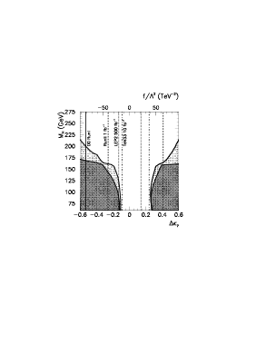
FIG. 2.: Excluded region in the $\Delta\kappa_{\gamma}\times M_{H}$ plane for an integrated luminosity of 100 pb^-1, and for scenarios $(ii)$ (clear shadow) and $(iii)$ (dark shadow). The present and future bounds on $\Delta\kappa_{\gamma}$ are also shown (see text for details).

$M_{H}$ (GeV)		100	150	200	250
$\ell\,\nu\,\gamma\,\gamma$	RunI	($-41$ — 74)	($-83$ — 113)	($<-200$ — $>200$)	$<-200$— $>200$
	RunII	($-13$ — 36)	($-22$ — 46)	($-57$ — 135)	($-195$ — $>200$)
	TeV33	($-3.8$ — 8)	($-4.8$ — 20)	($-28$ — 60)	($-45$ — 83)
$j\,j\,\gamma\,\gamma$	RunI	($-20$ — 49)	($-26$ — 64)	($-96$ —$>100$)	($<-100$ — $>100$)
	RunII	($-8.4$ — 26)	($-11$ — 31)	($-36$ — 81)	($-64$ — $>100$)
	TeV33	($-4.2$ — 6.5)	($-4.5$ — 12)	($-19$ — 40)	($-28$ — 51)

TABLE I.: Allowed range of $f/\Lambda^{2}$ in TeV^-2 at 95% CL, assuming the scenario $(i)$ ($f_{BB}=f_{WW}\gg f_{B},f_{W}$) for the different final states, and for different Higgs boson masses for an integrated luminosity of 100 pb^-1.

REFERENCES

- [1] K. Hagiwara, H. Hikasa, R. D. Peccei and D. Zeppenfeld, Nucl. Phys. B282, 253 (1987).
- [2] C. J. C. Burguess and H. J. Schnitzer, Nucl. Phys. B228, 464 (1983); C. N. Leung, S. T. Love and S. Rao, Z. Phys. 31, 433 (1986); W. Buchmüller and D. Wyler, Nucl. Phys. B268, 621 (1986).
- [3] A. De Rujula, M. B. Gavela, P. Hernandez and E. Masso, Nucl. Phys. B384, 3 (1992); A. De Rujula, M. B. Gavela, O. Pene and F. J. Vegas, Nucl. Phys. B357, 311 (1991).
- [4] K. Hagiwara, S. Ishihara, R. Szalapski and D. Zeppenfeld, Phys. Lett. B283, 353 (1992); idem, Phys. Rev. D48, 2182 (1993); K. Hagiwara, T. Hatsukano, S. Ishihara and R. Szalapski, Nucl. Phys. B496, 66 (1997).
- [5] For a review see: T. Yasuda, report FERMILAB–Conf–97/206–E, and hep–ex/9706015.
- [6] F. Abe et al., CDF Collaboration, Phys. Rev. Lett. 74, 1936 (1995); idem 74, 1941 (1995); idem 75, 1017 (1995); idem 78, 4536 (1997).
- [7] S. Abachi et al., DØ Collaboration, Phys. Rev. Lett. 75, 1023 (1995); idem 75, 1028 (1995); idem 75, 1034 (1995); idem 77, 3303 (1996); idem 78, 3634 (1997); idem 78, 3640 (1997).
- [8] B. Abbott et al., DØ Collaboration, Phys. Rev. Lett. 79, 1441 (1997).
- [9] For a review see: Z. Ajaltuoni et al., “Triple Gauge Boson Couplings”, in Proceedings of the CERN Workshop on LEPII Physics, edited by G. Altarelli, T. Sjöstrand, and F. Zwirner, CERN 96–01, Vol. 1, p. 525 (1996).
- [10] T. Barklow et al., Summary of the Snowmass Subgroup on Anomalous Gauge Boson Couplings, to appear in the Proceedings of the 1996 DPF/DPB Summer Study on New Directions in High-Energy Physics, June 25 — July 12 (1996), Snowmass, CO, USA.
- [11] D. Amidei et al., Future Electroweak Physics at the Fermilab Tevatron: Report of the TeV–2000 Study Group, preprint FERMILAB-PUB-96-082 (1996).
- [12] K. Hagiwara, R. Szalapski and D. Zeppenfeld, Phys. Lett. B318, 155 (1993).
- [13] B. Abbott et al., DØ Collaboration, FERMILAB-CONF-97/325-E, contribution to the Lepton-Photon Conference, Hamburg, July 1997.
- [14] K. Hagiwara, and M. L. Stong, Z. Phys. C62, 99 (1994); B. Grzadkowski, and J. Wudka, Phys. Lett. B364, 49 (1995); G. J. Gounaris, J. Layssac and F. M. Renard, Z. Phys. C65, 245 (1995); G. J. Gounaris, F. M. Renard and N. D. Vlachos, Nucl. Phys. B459, 51 (1996).
- [15] S. M. Lietti, S. F. Novaes and R. Rosenfeld, Phys. Rev. D54, 3266 (1996); F. de Campos, S. M. Lietti, S. F. Novaes and R. Rosenfeld, Phys. Lett. B389, 93 (1996).
- [16] A. Stange, W. Marciano, and S. Willenbrock, Phys. Rev. D49, 1354 (1994); Phys. Rev. D50, 4491 (1994).
- [17] J. F. Gunion, H. E. Haber, G. Kane, S. Dawson, The Higgs Hunter’s Guide (Addison–Wesley, 1990).
- [18] R. Keiss, Z. Kunszt, and W. J. Stirling, Phys. Lett. B253, 269 (1991); J. Ohnemus and W. J. Stirling, Phys. Rev. D47, 336 (1992); U. Baur, T. Han, N. Kauer, R. Sobey, and D. Zeppenfeld, Phys. Rev. D56, 140 (1997).
- [19] V. Barger, T. Han , D. Zeppenfeld, and J. Ohnemus, Phys. Rev. D41, 2782 (1990).
- [20] T. Stelzer and W. F. Long, Comput. Phys. Commun. 81, 357 (1994).
- [21] H. Murayama, I. Watanabe and K. Hagiwara, KEK report 91-11 (unpublished).
- [22] A. D. Martin, W. J. Stirling, R. G. Roberts Phys. Lett. B354, 155 (1995).
- [23] O. Helene, Nucl. Instr. and Meth. 212, 319 (1983).