1 Introduction.

Our aim is to study the various ways to describe the $\rho^{0}$ meson in order to find an optimum modelling able to account most precisely for the known features of the physics involving this meson. This is mainly motivated by the fact that a precise knowledge of its properties is of fundamental importance in several fields of particle physics. It is important to emphasise that our philosophy is to look for the simplest models as these are the most useful in application to other systems, due to their ease of implementation. Naturally, such models should, as much as possible, respect basic general principles such as gauge invariance and unitarity. One must keep in mind that any parameters quoted for a given model are relevant only to that model. Indeed, a study of the model-dependence of resonance parameters is one of the principal goals of this work. It should also be noted that while each of these models is related to some underlying effective field theory through an effective Lagrangian, the models we are using here are simple amplitudes arising from an assumption of almost complete $s$-channel resonance saturation. The appropriateness of this assumption away from the resonance region can only be judged by quantitative studies of higher order (e.g., loop) effects in the corresponding effective field theories. While this is clearly a very important task, it is not our concern here and will not be considered further.

For this purpose, we study the strong interaction corrections to one-photon mediated processes in the low energy region where QCD is non-perturbative. To do this we shall look at two related processes, $e^{+}e^{-}\rightarrow\pi^{+}\pi^{-}\;$and $e^{+}e^{-}\rightarrow\mu^{+}\mu^{-}\;$. The effect of the strong interaction is obvious in the first reaction and provides a large enhancement to the production of pions in the vector meson resonance region [2, 3, 4, 5]. This enhancement, relative to what would be expected for a structureless, pointlike pion, is reflected in the deviation of the pion form factor, $F_{\pi}(q^{2})$, from $1$, and is primarily associated with the $\rho$ meson (where $q_{\mu}$ is the four momentum of the virtual photon). This form factor is successfully modelled in the intermediate energy region using the vector meson dominance (VMD) model [6]. VMD assumes that the photon interacts with physical hadrons through vector mesons and it is these mesons that give rise to the enhancement, through their resonant (possessing a complex pole) propagators of the form

$$D_{\mu\nu}(q^{2})=\frac{-g_{\mu\nu}}{q^{2}-{m}_{V}^{2}+i{m}_{V}\Gamma_{V}(q^{2})},$$ (1)

where ${m}_{V}$ and $\Gamma_{V}$ are the (real valued) mass and the momentum-dependent width. (Here we have included only that part of the propagator which survives when coupled to conserved currents.)

Traditionally, VMD assumes that all photon–hadron coupling is mediated by vector mesons. However, from an empirical point of view, one has the freedom, motivated by Chiral Perturbation Theory (ChPT) to include other contributions to such interactions. For instance, in a fit to $F_{\pi}(q^{2})$ [7], it was shown that a non-resonant photon–hadron coupling can be accommodated merely by shifting the mass and width of the $\rho^{0}$ by about 10 MeV. Thus, the values extracted from $F_{\pi}(q^{2})$ for the $\rho$ mass, $m_{\rho}$, and width, $\Gamma_{\rho}$, are model-dependent and in quoting values for them, the model used should be clearly stated. We note in passing that to define vector meson masses and widths in a process-independent way, one should refer to the location of the corresponding complex pole in the S-matrix. One should, however, bear in mind that alternate, and more traditional definitions of the mass and width not tied to the location of the S-matrix pole (for example a definition of $m_{\rho}^{2}$ as that value of $q^{2}$ for which the $P$–wave $\pi\pi$ phase shift passes through $90^{\circ}$) are in general specific to the process employed in the definition. The process-dependence of such alternate mass and width definitions has in fact led a number of authors to advocate using the S-matrix pole position to provide a process-independent definition of the $Z^{0}$ mass and width in the Standard Model[8].

Naturally, VMD can be applied to many other systems. We can consider the process $\eta^{\prime}/\eta\rightarrow\pi^{+}\pi^{-}\gamma$ taking place through a combination of resonant (such as $\eta^{\prime}/\eta\rightarrow\rho\gamma\rightarrow\pi^{+}\pi^{-}\gamma$) and non-resonant channels. In this manner an acceptable fit to data can be achieved with a range of combinations for the $\rho$ parameters and non-resonant terms [7, 9]. Recent interest in this process has centred on the non-resonant term, which, if it arises from anomalous box and triangle diagrams, provides a possible test of QCD [10, 11, 12]. However, to determine the size of any non-resonant contribution, the resonant meson parameters need to be well fixed [7, 9], and thus $F_{\pi}(q^{2})$ well understood. This is one of the main aims of this paper.

We thus turn our attention to $e^{+}e^{-}\rightarrow\mu^{+}\mu^{-}\;$. In modelling the strong interaction correction to the photon propagator, VMD assumes that the strong interaction contribution is saturated by the spectrum of vector meson resonances [13]. Therefore, in principle, we can extract information on the vector meson parameters (independently of the $e^{+}e^{-}\rightarrow\pi^{+}\pi^{-}\;$fit) without having to worry about non-resonant processes. However, as the vector mesons enter in $e^{+}e^{-}\rightarrow\mu^{+}\mu^{-}\;$with an extra factor of $\alpha$ compared with $e^{+}e^{-}\rightarrow\pi^{+}\pi^{-}\;$, their contributions are considerably suppressed, making their extraction difficult. For this reason, we shall perform a simultaneous fit to both sets of data, in order to impose the best possible constraint on the vector meson parameters, and see if existing muon data are already precise enough in order to constrain the $\rho^{0}$ parametrisation.

Another way to constrain the descriptions of the $\rho^{0}$ meson is to compare the strong interaction $\pi\pi$ phase obtained using the various VMD parametrisations determined in fitting $e^{+}e^{-}\rightarrow\pi^{+}\pi^{-}\;$with the corresponding phase [14] obtained using $\pi\pi$ scattering data and the general principles of quantum field theory, as well as the near–threshold predictions of ChPT. This happens to be more fruitful and conclusive in showing how VMD should be dealt with in order to reach an agreement with a large set of data and with the basic principles of quantum field theory.

The hadronic dressing of the photon propagator (the one-photon irreducible self-energy $\Pi^{\rm had}(q^{2})$) is also of interest for another reason. The anomalous magnetic moment of the muon can now be measured to such accuracy [15] that the strong interaction correction is important [16]. This needs to be completely understood if one is to look for physics beyond the Standard Model in this quantity. At present the correction is inferred from $\sigma(e^{+}e^{-}\rightarrow$ hadrons) using dispersion theory and the optical theorem or estimated with hadronic models (which, being non-perturbative, are difficult to use). The process $e^{+}e^{-}\rightarrow\mu^{+}\mu^{-}\;$allows for a direct examination of the strong interaction modification to the photon propagator. Ideally we would obtain the low energy corrections to the photon propagator experimentally, and be able to use QCD perturbatively for higher energies (though the threshold above which we can ignore non-perturbative effects is difficult to determine [17]). The $\phi$ meson has already been seen in $e^{+}e^{-}\rightarrow\mu^{+}\mu^{-}\;$[2, 5]. It is only noticeable around the pole region where, due to its small width (4.4 MeV), it produces a sharp peak easily seen in the available data. The large width of the $\rho$ further suppresses the $\rho$ and $\omega$ contributions.

The outline of the present work is as follows. In section 2 we describe the various formulations of the VMD assumption and the unitarisation procedure; we also discuss the phase definition relevant for our purpose. The fit procedure is sketched in section 3 and implemented in section 4. Comparison with the isospin 1 $P$–wave $\pi\pi$ phase shift deduced from $\pi\pi$ scattering theory is the subject of section 5, while in section 6 we give the near–threshold parameter values that are deduced from our fits of the $e^{+}e^{-}\rightarrow\pi^{+}\pi^{-}\;$cross section and they are compared to predictions and to other experimental determinations. The results obtained are discussed in section 7 where we present our optimal fit for the $\rho^{0}$ parameters and the model which accounts for its properties the most appropriately. Finally, we summarise our conclusions in section 8.

2 Vector meson models

We shall now provide a description of the various models we will use to fit the data for both $e^{+}e^{-}\rightarrow\pi^{+}\pi^{-}\;$and $e^{+}e^{-}\rightarrow\mu^{+}\mu^{-}\;$. The cross-section for $e^{+}e^{-}\rightarrow\pi^{+}\pi^{-}\;$is given by (neglecting the electron mass)

$$\sigma=\frac{\pi\alpha^{2}}{3}\frac{(q^{2}-4m_{\pi}^{2})^{3/2}}{(q^{2})^{5/2}}|F_{\pi}(q^{2})|^{2},$$ (2)

where the form factor, $F_{\pi}(q^{2})$ is determined by the specific model. Similarly, $F_{\mu}(q^{2})$ is defined to be the form factor for the muon, and the cross-section for $e^{+}e^{-}\rightarrow\mu^{+}\mu^{-}\;$is given by,

$$\sigma=\frac{4\pi\alpha^{2}}{3q^{2}}\sqrt{1-\frac{4m_{\mu}^{2}}{q^{2}}}\left(1+\frac{2m_{\mu}^{2}}{q^{2}}\right)|F_{\mu}(q^{2})|^{2}.$$ (3)

It is worth noting that these standard definitions of $F_{\pi}(q^{2})$ and $F_{\mu}(q^{2})$ contain all non-perturbative effects, including for example the photon vacuum polarisation, since Eqs. (2) and (3) are written assuming a perturbative photon propagator.

We shall use VMD, the Hidden Local Symmetry model of Ref. [18] (hereafter refered to as HLS) and what we will refer to as the WCCZW model (a phenomenological modification of the general framework of Ref. [19], based on work by Birse[20]), as well as modifications of these models, which cover or underlie a large class of effective Lagrangians describing the interactions of photons, leptons and pseudoscalar and vector mesons. Birse [20] has shown that typical effective theories involving vector mesons based on a Lagrangian approach, such as “massive Yang-Mills” and “hidden gauge” (i.e., HLS-type) are equivalent. We therefore consider our following examination to be reasonably comprehensive. Numerical approaches to the strong interaction in the vector meson energy region [21], which are not based on an effective Lagrangian involving meson degrees of freedom do not yet possess the required calculational accuracy for our task.

2.1 VMD

The simplest model is VMD itself. As has been discussed in detail elsewhere [6, 22, 23] VMD has two equivalent formulations, which we shall call VMD1 and VMD2. The VMD1 model has a momentum-dependent coupling between the photon and the vector mesons and a direct coupling of the photon to the hadronic final state. The resulting form factor is (to leading order in isospin violation and $\alpha=e^{2}/4\pi$):

$$F_{\pi}^{\rm VMD1}(q^{2}) = 1-g^{\rm VMD1}_{\rho\gamma}(q^{2})\frac{g_{\rho\pi\pi}}{[q^{2}-m^{2}_{\rho}+im_{\rho}\Gamma_{\rho}(q^{2})]}$$ (4)

$$-g^{\rm VMD1}_{\omega\gamma}(q^{2})\frac{1}{[q^{2}-m^{2}_{\omega}+im_{\omega}\Gamma_{\omega}(q^{2})]}Ae^{i\phi_{1}}.$$

The $\omega$ enters into the isospin 1 $e^{+}e^{-}\rightarrow\pi^{+}\pi^{-}\;$interaction with an attenuation factor specified by the pure real $A$ and the Orsay phase, $\phi$ [24]; these can be extracted from experiment For VMD2 we have,

$$F_{\pi}^{\rm VMD2}(q^{2})=-g^{\rm VMD2}_{\rho\gamma}\frac{g_{\rho\pi\pi}}{[q^{2}-m^{2}_{\rho}+im_{\rho}\Gamma_{\rho}(q^{2})]}-g^{\rm VMD2}_{\omega\gamma}\frac{1}{[q^{2}-m^{2}_{\omega}+im_{\omega}\Gamma_{\omega}(q^{2})]}Ae^{i\phi_{2}}.$$ (5)

The form factor for the muon, however, in both representations (i=1, 2) is given by

$$F_{\mu}^{\rm VMDi}=1+\sum_{V}e^{2}[g_{V\gamma}^{\rm VMDi}(q^{2})]^{2}\frac{1}{q^{2}-{m}_{V}^{2}+i{m}_{V}\Gamma_{V}(q^{2})}\frac{1}{q^{2}},$$ (6)

which is consistent with previous expressions for the $\phi$-meson [2, 25]. In higher order (i.e., in all but the minimal VMD picture) there will also be contributions from non–resonant processes (such as two–pion loops), but these are expected to be small near resonance and the non–resonant background is, in any case, fitted in extractions of resonance parameters from the experimental data. The photon–meson coupling, $eg_{V\gamma}$ is fixed in VMD2 by [25]

$$\Gamma_{V\rightarrow e^{+}e^{-}}=\frac{4\pi\alpha^{2}}{3{m}_{V}^{3}}g^{2}_{V\gamma}.$$ (7)

The (dimensionless) universality coupling, $g_{V}$, is then defined by

$$g_{V\gamma}^{\rm VMD2}={m}_{V}^{2}/g_{V}$$ (8)

for VMD2 [22, 24]. This coupling (and universality) has been most closely studied for the $\rho$ meson. A gauge-like argument [6, 26] suggests that the $\rho$ couples to all hadrons with the same strength $g_{V}$ (universality) [22]. However, experimentally, universality is observed to be not quite exact [27], so we introduce the quantity $\epsilon$ (to be fitted) through

$$g_{\rho\gamma}^{\rm VMD2}=\frac{{m}_{\rho}^{2}}{g_{\rho\pi\pi}}(1+\epsilon)$$ (9)

where $g_{\rho\pi\pi}$ and $\epsilon$ are to be extracted from the fit to $e^{+}e^{-}\rightarrow\pi^{+}\pi^{-}\;$. For VMD1, it can be seen that the photon-meson coupling results from replacing the mass term in Eq. (8) by $q^{2}$[6, 26]. In this case Eq (9) should be replaced by

$$g_{V\gamma}^{\rm VMD1}=\frac{q^{2}}{g_{\rho\pi\pi}}(1+\epsilon)~{}~{}.$$ (10)

One can easily see that in VMD1 the hadronic correction to the photon propagator goes like $q^{4}$ and so maintains the photon pole at $q^{2}=0$. For VMD2, it is not obvious [28] that gauge invariance is maintained until one considers the inclusion of a bare photon mass term in the VMD Lagrangian that exactly cancels the hadronic correction at $q^{2}=0$. This argument [29] assumes a $\rho-\gamma$ coupling of the form $em_{\rho}^{2}/g_{\rho}$ and a bare photon mass ($e^{2}m_{\rho}^{2}/g_{\rho}^{2}$) (the calculation is presented in detail in Ref. [6]). In the presence of a finite $\epsilon$, as in Eq. (9), gauge invariance is similarly preserved by including a photon mass term ($e^{2}m_{\rho}^{2}(1+\epsilon)^{2}/g_{\rho}^{2}$) leading to a massless photon as expected [30].

The presence of a finite $\epsilon$ does affect the charge normalisation condition $F_{\pi}(0)=1$, but this is merely an artifact of the simple $\rho$ propagators we are considering. A more sophisticated version, such as used by Gounaris and Sakurai [31] which fully accounts for below threshold behaviour, maintains $F_{\pi}(0)=1$ in the presence of $\epsilon\neq 0$. One could, alternatively, include an $s$ dependence to $\epsilon$ such that $\epsilon(0)=0$. In any case, the phenomenological significance for the physical $\rho$ (for the data region we are fitting) is negligible, we achieve an excellent fit to the data with the simple form we use but are not advocating its use outside this fitting region, namely above the two-pion threshold.

The choice of the detailed form of the momentum-dependent width, $\Gamma_{V}(q^{2})$, allows one certain amount of freedom. As the complex poles of the amplitude are field-choice and process-independent properties of the S-matrix [32] one could, on the one hand, expand the propagator as a Laurent series in which the non-pole terms go into the background [33]. Alternatively, one could use the $l-$wave momentum-dependent width to account for the branch point structure of the propagator above threshold ($q^{2}=4m_{\pi}^{2}$) [7, 34, 31]. This form for the momentum dependent width arises naturally from the dressing of the $\rho$ propagator in an appropriate Lagrangian based model (see Sec. 5.1 of Klingl et al. for a detailed treatment [27]) and, for such models, is given by

$$\Gamma_{\rho}(q^{2})=\Gamma_{\rho}\left[\frac{p_{\pi}(q^{2})}{p_{\pi}(m_{\rho}^{2})}\right]^{3}\left[\frac{m_{\rho}^{2}}{q^{2}}\right]^{\lambda/2},$$ (11)

introducing the fitting parameters $\Gamma_{\rho}$ (the width of the $\rho^{0}$ meson at $q^{2}=m_{\rho}^{2}$) and $\lambda$, which generalises the usual $l$–wave expression [7] to model the fall–off of the $\rho$ mass distribution; the usual case (i.e. $\lambda=1$) is associated with a $\rho$ coupling to pions of the form $g_{\rho\pi\pi}\rho^{\mu}(\pi^{+}\partial_{\mu}\pi^{-}-\pi^{-}\partial_{\mu}\pi^{+})$, with $g_{\rho\pi\pi}$ independent of $q^{2}$, as shown in Ref. [27]. Note that the parameters $\lambda$, $m_{\rho}$ and $\Gamma_{\rho}$ are model-dependent (as we see in the tables of results, different models yield different values for these parameters). Note that in Eq. (11) we have defined the pion momentum in the centre of mass system

$$p_{\pi}(q^{2})=\frac{1}{2}\sqrt{q^{2}-4m_{\pi}^{2}}.$$ (12)

Before closing this section, let us remark that the pion form factor associated with VMD1 (Eq. (4)) fulfills automatically the condition $F_{\pi}(0)=1$ whatever the value of the universality violating parameter $\epsilon$ (see Eq. (10)). This is not the case for the pion form factor associated with VMD2 (Eq. (5)), as can be seen from Eqs. (5) and (9). Here, we will concern ourselves exclusively with fitting data in the above threshold region and simply note it is a relatively straightforward matter to generalise the VMD models considered to satisfy this condition. Detailed considerations of this issue are left for future work.

While of course VMD1 and VMD2 are equivalent in the limit of exact universality if one keeps all diagrams, (i.e., if one works to infinite order in perturbation theory), in any practical calculation one cannot do that and so, in practice, these two expressions of VMD can give different predictions in general, even if exact universality is imposed. Moreover, if one releases (as we do) this last constraint, equivalence of VMD1 and VMD2 is not guaranted, even in principle.

2.2 The HLS Model

The Hidden Local Symmetry (HLS) model [6, 18] introduces a parameter $a$ for the $\rho$ meson within a dynamical symmetry breaking model framework. This $a$ relates the constant $g_{\rho\pi\pi}$ to the universality coupling $g_{\rho}$ via

$$g_{\rho\pi\pi}=\frac{ag_{\rho}}{2}.$$ (13)

The resulting form factor for the pion is

$$F_{\pi}(q^{2})=-\frac{a}{2}+1-g_{\rho\gamma}\frac{g_{\rho\pi\pi}}{(q^{2}-m_{\rho}^{2}+im_{\rho}\Gamma_{\rho}(q^{2}))}-g_{\omega\gamma}\frac{1}{q^{2}-m^{2}_{\omega}+im_{\omega}\Gamma_{\omega}(q^{2})}Ae^{i\phi}.\\$$ (14)

The original HLS model preserved isospin symmetry and so did not include the $\omega$. Isospin breaking has recently been studied in a generalisation of the HLS model [35], however, here we have for simplicity employed the same $\omega$ terms as used for VMD. The relations equivalent to Eqs. (8) and (9) for the $\rho$ meson are now

$$g_{\rho\gamma}=\frac{a}{2}\frac{m_{\rho}^{2}}{g_{\rho\pi\pi}}=\frac{m_{\rho}^{2}}{g_{\rho}}\ .$$ (15)

We see that setting $a=2$ reproduces VMD2 in the limit of exact universality. However, we wish to keep $a$ as a free parameter which we can fit to the data. Note that in the HLS model universality violation and the existence of a non–resonant coupling $\gamma\pi^{+}\pi^{-}$ are related. Note also that universality violation can be introduced in the HLS model without violating the constraint $F_{\pi}(0)=1$, in a natural way.

The muon form factor for the HLS model is exactly the same as for VMD2 (see Eqs. (6) and (15)).

2.3 WCCWZ Lagrangian

Birse has recently discussed [20] the pion form factor arising from the WCCWZ Lagrangian [19] in which the vector and axial vector fields transform homogeneously under non-linear chiral symmetry. The scheme imposes no constraints on the couplings of the spin 1 particles beyond those of approximate chiral symmetry. Birse’s version of the form factor is (isospin violation is not considered)

$$F_{\pi}(q^{2})=1-\frac{g_{1}f_{1}}{f_{\pi}^{2}}\frac{q^{4}}{q^{2}-m^{2}_{\rho}+im_{\rho}\Gamma_{\rho}(q^{2})}+\frac{f_{2}}{f_{\pi}^{2}}q^{2},$$ (16)

where the first two terms on the RHS are those arising from the WCCWZ Lagrangian. The $q^{4}$ piece grows at large $q^{2}$ in a way incompatible with QCD predictions (for a discussion of matching the asymptotic prediction to a low energy model see Geshkenbein [36]). The $f_{2}$ contribution has been added by Birse to modify this high energy behaviour toward that expected in QCD. To this end, Birse sets

$$f_{2}=g_{1}f_{1}=\frac{f_{\pi}^{2}}{m^{2}_{\rho}}$$ (17)

and recovers the universality limit of the form factor in which VMD1 and VMD2 are equivalent (in the zero width approximation). Note that a $q^{2}$-dependence of the non-resonant background is what one would, in general, obtain from the WCCWZ framework, implemented in its most general form, which relies only on the symmetries of QCD. In constructing a phenomenological implementation we have, however, simplified the most general form, adding what amounts to a minimal $q^{2}$-dependence to the background term of VMD1. The resulting form factor, which we will refer to as the WCCWZ model, is then

$$F_{\pi}(q^{2})=1+bq^{2}-\frac{g_{\rho\gamma}^{\rm WCCWZ}(q^{2})g_{\rho\pi\pi}}{q^{2}-m^{2}_{\rho}+im_{\rho}\Gamma_{\rho}(q^{2})}-g_{\omega\gamma}\frac{Ae^{i\phi}}{q^{2}-m_{\omega}^{2}+im_{\omega}\Gamma_{\omega}(q^{2})},$$ (18)

where we keep $b$ as an independent parameter to be fit.

The WCCWZ model, thus, has one more free parameter than VMD1. We have added the $\omega$ contribution as above for all other models. The muon form factor is exactly the same as for VMD1 (see Eq. (6)).

It is important to note that the WCCWZ model allows one to have a non–resonant term which can be mass dependent, cf., VMD2 which carries only resonant contributions or VMD1 or the HLS models which both exhibit only constant non–resonant contributions to the pion form factor. The expression in Eq. (18) exhibits an unphysical high energy behaviour; however, as we are only interested in the pion form factor at low energies (below 1 GeV), this feature is not relevant. Of course, one can consider that such a polynomial structure at low energies represents an approximation in the resonance region to a function going to zero at high energies .

The model VMD2 contains only resonant contributions, whereas VMD1, HLS and WCCWZ also contain a non–resonant part. For VMD1 and HLS, this term is constant (i.e., pointlike) as in standard lowest order QED. We shall frequently refer to this term as a direct $\gamma\pi\pi$ contribution or coupling. In the case of WCCWZ, this non–resonant term also contains a $q^{2}$–dependent piece which clearly indicates a departure from a point–like coupling; nevertheless, we shall also refer to it as a direct $\gamma\pi\pi$ coupling for convenience.

2.4 Elastic Unitarity

When $\lambda\neq 1$ the pion form factor described above in the VMD, HLS and WCCWZ models does not in general exactly fulfill unitarity. This is because one employs simultaneously a bare, undressed $\rho^{0}\pi^{+}\pi^{-}$ coupling (given by the tree–level coupling, $g_{\rho\pi\pi}$) and a dressed $\rho^{0}$ propagator, as signalled by the presence of a momentum–dependent width in Eq. (11) (see, e.g., Ref. [27]). To see why this generally creates a problem with unitarity, consider the $\pi\pi\rightarrow\pi\pi$ $P$–wave $I=1$ strong interaction amplitude. It is most convenient here to employ the $N/D$ formalism for the amplitude T (see, e.g., Ref. [38]).

It has been known for some time that the $I=l=1$ $\pi\pi$ amplitude is consistent with being purely elastic from threshold up to $\simeq 1$ GeV [39, 40, 41]. Therefore, in this region, we can write

$$S=1+2ip_{\pi}T=\exp{[2i\delta^{1}_{1}]}$$ (19)

from which it follows that

$$T=\displaystyle\frac{\exp{[i\delta^{1}_{1}]}~{}\sin\delta^{1}_{1}}{p_{\pi}}=\displaystyle\frac{N}{D}$$ (20)

where $p_{\pi}$ has been defined in Eq. (12). In the region where the $\rho^{0}$ meson essentially saturates the $I=l=1$ $\pi\pi$ wave, the $D$ function may be approximated by the inverse $\rho^{0}$ propagator ($s\equiv q^{2}$),

$${D}(s)=s-m_{\rho}^{2}+im_{\rho}\Gamma_{\rho}(s)~{}~{}~{}.$$ (21)

$D$ in Eq. (20), is an analytic function of $s$, having as sole singularity in the physical sheet a cut along the real axis ($s\geq 4m_{\pi}^{2}$). Correspondingly, the singularities of the $N$ function on the physical sheet are all located on the real axis at negative values of $s$ (for example, singularities produced by exchanges in the $t$ and $u$ channels projected out onto the $P$–wave). Moreover $N$ is real on the real axis above threshold ($4m_{\pi}^{2}$). It should also be noted that the $N$ and $D$ functions in Rel. (20), are defined up to a multiplicative arbitrary function $f(s)$, meromorphic in the complex $s$–plane. The choice used in Eq. (21) corresponds to a particular choice of $f(s)$. Put simply, the content of Eq. (21) is that the phase of $D$ is well approximated by the phase of the $\rho^{0}$ propagator in the vector meson resonance region.

As a consequence of unitarity and analyticity, $N$ is connected with the discontinuity of $D$ across the physical region ($s\geq 4m_{\pi}^{2}$) through

$$\lim_{\varepsilon\rightarrow 0}~{}~{}[{D}(s-i\varepsilon)-{D}(s+i\varepsilon)]=2ip_{\pi}{N}(s),$$ (22)

which gives [7],

$$N(s)=-\frac{m_{\rho}\Gamma_{\rho}(s)}{p_{\pi}}.$$ (23)

As the $N$ function is closely connected with the $\rho\pi^{+}\pi^{-}$ vertex, this last relation implies some dressing of the vertex coupling. This relation illustrates the effect of the parameter $\lambda$, whose role is simply to model the contributions from the left–hand singularities of the scattering amplitude. Then using Eqs. (21 – 23), it is easy to check that $|S|=1$ is automatically satisfied in the physical region below $\simeq 1$ GeV, as required by unitarity, and that

$$\tan{\delta^{1}_{1}}=\displaystyle\frac{m_{\rho}\Gamma_{\rho}(s)}{m_{\rho}^{2}-s}~{}~{}.$$ (24)

Thus from Eq. (24) we can conclude that $\delta^{1}_{1}$ can be well approximated by the negative of the $\rho$ propagator phase, if one considers resonant contributions only.

One can then show[7] that unitarity can be restored to the model treatments above by replacing the coupling $g_{\rho\pi\pi}$ in Eqs. (4), (5), (14) and (18) with

$$G_{\rho}(q^{2})=\displaystyle\sqrt{6\pi\frac{m_{\rho}q}{p_{\pi}^{3}(q^{2})}\Gamma_{\rho\rightarrow\pi^{+}\pi^{-}}(q^{2})}$$ (25)

where $q\equiv\sqrt{q^{2}}$. This replacement leads to the unitarised versions of our VMD models. The connection between this “dressed” vertex function and $g_{\rho\pi\pi}$ gives (cf., Eq. (4.16) of Ref. [27])

$$g_{\rho\pi\pi}=\sqrt{6\pi\frac{m_{\rho}^{2}}{p_{\pi}^{3}(m_{\rho}^{2})}\Gamma_{\rho}},$$ (26)

from which we see that

$$g_{\rho\pi\pi}=G_{\rho}(m_{\rho}^{2}).$$ (27)

It should be noted that the left hand side of Eq. (25) becomes constant – and then coincides with $g_{\rho\pi\pi}$ – if and only if $\lambda=1$ (see Eq. (11)). Therefore, if $\lambda\equiv 1$ Eqs. (4), (5), (14) and (18) are already unitarised and the singularities of $N$ (see Eq. (23)) are simply a branch point going from $s=0$ to $-\infty$, where $s=0$ is also a pole.

Strictly speaking, one should similarly unitarise the $\omega$ contribution. However, since the $\omega$ is very narrow, its contributions are significant only over a very limited range of $q^{2}$. Hence, it is sufficient to employ a constant $\omega\pi\pi$ coupling (or equivalently, constant $A$) in Eqs. (4), (5), (14) and (18). The value of $A$ may be determined from the branching fraction of $\omega\rightarrow\pi^{+}\pi^{-}$, as was done in Ref. [7] or fitted. Therefore, the only actual free parameter in the $\omega$ contribution is the Orsay phase, $\phi$. This will in no way affect the description of the $\rho^{0}$ itself, which is our main concern. Finally, unitarisation clearly does not affect the expressions for the muon form factor.

The unitarised version of VMD2 coincides with the phenomenological model called M₂ in Refs. [7, 9]. Here, however, we shall fit $g_{\rho\gamma}$ and then BR$(\rho^{0}\rightarrow e^{+}e^{-})$, which was previously simply fixed at its PDG [42] value . The unitarised version of the HLS model is close to the phenomenological model M₃ of Ref. [9].

We note that the non–resonant term introduced by VMD1 and HLS models is constant at leading order whereas M₁ of Refs. [7, 9] has a $q^{2}$–dependent non–resonant piece. In this respect the WCCWZ model is close to M₁.

2.5 Phase of $F_{\pi}(q^{2})$ and Phase of the $\pi\pi\rightarrow\pi\pi$ Amplitude

From general properties of field theory (mainly, unitarity and $T$–invariance), it can be shown [43] that for $s\equiv q^{2}$ real above threshold, we have

$$F_{\pi}(s)=\exp{[2i\delta_{1}^{1}]}~{}~{}F_{\pi}^{*}(s)~{}~{}~{},$$ (28)

up to the first open inelastic threshold. Using Eq. (19) and Eq. (20) – which defines the $N/D$ formalism–, this relation gives [43]

$$F_{\pi}(s)=\frac{1}{D(s)}~{}~{},$$ (29)

where $D(s)$ has been defined by its general properties in the preceding section. In order that $F_{\pi}(0)=1$, the $D$ function should fulfill $D(0)=1$. The functions $D$ appearing here and in Eq (20) can be chosen identical without any loss of generality. It is obvious from Eq. (29) that $F_{\pi}(s)$ carries the same phase as $1/D(s)$ and as the $\pi\pi\rightarrow\pi\pi$ amplitude.

The identification of the function $D$ in Eq. (20) with a resonance propagator, namely the $\rho^{0}$ meson (see Eq. (21)), would be motivated in the present case by the fact that the amplitude is dominated by a single resonance (the $\rho^{0}$ meson itself) [39, 40, 41]. This does not mean that higher mass resonances, which surely exist [4, 44], have a (strictly) zero contribution in our mass range, but simply that their magnitude is negligible compared to that of the $\rho$ meson. In this case, the Breit-Wigner parametrisation is flexible enough in order to absorb these small contributions into a correspondingly small change of the parameter values with respect to their (unknown) “true” values. This is also valid for a possible small non-resonant hadronic contribution to the amplitude.

As far as hadronic contributions to the pion form factor are concerned, there are also contributions from the $\omega$ and $\phi$ mesons. Because of their small width, we can add their contributions to $F_{\pi}(s)$; this will produce departures from Eq. (29), however always in very limited invariant mass interval. Moreover, they do not contribute to the $I=l=1$ $\pi\pi$ phase shift for obvious reasons.

Putting aside the question of $\omega$ and $\phi$ mesons for the reasons just given, it remains to recall that there is a direct $\gamma\pi\pi$ contribution to the form factor present in the models VMD1, HLS, and WCCWZ, whereas VMD2 has no such contribution. These additional direct contributions, which are constant for VMD1 and HLS models, modify the total phase near threshold where the hadronic ($\rho^{0}$) contribution is small in magnitude. Therefore, it is appropriate to take the full phase of $F_{\pi}(s)$, rather than the phase of the $\rho^{0}$ propagator only, which allows us to extract the exact behaviour of the $\pi\pi\rightarrow\pi\pi$ phase ($\delta_{1}^{1}$) in the threshold region.

3 Simultaneous Fits of $e^{+}e^{-}\rightarrow\pi^{+}\pi^{-}$ and $\mu^{+}\mu^{-}$ Data

Fitting the $e^{+}e^{-}$ data from threshold to about 1 GeV involves three well-known resonances, $\rho^{0}$, $\omega$ and $\phi$. As the last two are narrow, their parametrisation is relatively simple. But, due to its broadness, the $\rho^{0}$ meson has given rise to long standing problems of parametrisation (see Refs. [7, 34, 31] and previous references quoted therein). Moreover, as we have mentioned, one can ask whether experimental data require the existence of a non–resonant $\gamma\pi^{+}\pi^{-}$ coupling. The conclusion of Refs. [7, 9] is that data on $F_{\pi}(q^{2})$ alone are insufficient to answer this question. This is also relevant to the test of QCD proposed by Chanowitz [10, 11].

In addition to the mass and width, in the context of the class of models having widths of the form given in Eq. (11), one requires

only one additional parameter, $\lambda$, to define the $\rho$ shape. The resulting fit turns out to depend not only on the non-resonant coupling, but also on whether unitarisation is used or not. One approach [45] to this problem is to perform a simultaneous fit of all $e^{+}e^{-}\rightarrow\pi^{+}\pi^{-}$ data [4] and $e^{+}e^{-}\rightarrow\mu^{+}\mu^{-}$ data [46]. Indeed, if the data are precise enough, we could see a non–resonant coupling in $e^{+}e^{-}\rightarrow\pi^{+}\pi^{-}$, which will (of course) be small in $e^{+}e^{-}\rightarrow\mu^{+}\mu^{-}$. Therefore, from first principles, a simultaneous fit to both data allows us to decouple the $\rho$ from any non–resonant $\gamma\pi^{+}\pi^{-}$ coupling. Naturally, to be of any use in this, the $e^{+}e^{-}\rightarrow\mu^{+}\mu^{-}\;$data would have to be very good. Until recently relatively precise measurements were available only for the region around the $\phi$ mass [2, 5]. However, a new data set [46] collected by the olya collaboration is available and covers a large invariant mass interval from 0.65 GeV up to 1.4 GeV. We shall see shortly whether it is precise enough to constrain the $\rho$ parameters. Thus, the data sets which will be used for our fits are those collected by dm1, olya and cmd which are tabulated in [4] (for $e^{+}e^{-}\rightarrow\pi^{+}\pi^{-}\;$) and only the olya data of [46] for $e^{+}e^{-}\rightarrow\mu^{+}\mu^{-}\;$; these data sets do not cover the $\phi$ peak region.

4 Results of $e^{+}e^{-}$ data analysis

In all of the previously described models, except for WCCWZ, the fit to $e^{+}e^{-}\rightarrow\pi^{+}\pi^{-}$ and $e^{+}e^{-}\rightarrow\mu^{+}\mu^{-}$ data depends on only five parameters. The first four are the three $\rho$ meson parameters (${m}_{\rho}$, $\Gamma_{\rho}$ and $\lambda$) and the Orsay phase ($\phi$). These are common to both VMD and HLS. In the VMD models an additional parameter, $\epsilon$, has been introduced in order to account for universality violation (see Eqs. (9) and (10)), while in the HLS model this parameter is replaced by $a$ (see Eq. (15)). These last parameters allow us to fit the branching fraction $\rho^{0}\rightarrow e^{+}e^{-}$ within each model in a consistent way. The WCCWZ model depends on one additional parameter, $b$, which permits a more flexible form for the non–resonant contribution, as compared with the VMD1 or HLS models. Let us note that introducing $e^{+}e^{-}\rightarrow\mu^{+}\mu^{-}\;$in our fit procedure together with $e^{+}e^{-}\rightarrow\pi^{+}\pi^{-}\;$does not require further free parameters.

Generally speaking, the parameter named $A$ in the VMD models above determines the branching ratio Br$(\omega\rightarrow\pi^{+}\pi^{-})$ and should be set free since its value is strongly influenced by the data on $e^{+}e^{-}\rightarrow\pi^{+}\pi^{-}\;$we are fitting. However, in order to minimise the number of fit parameters at the stage when different models are still considered, we fix its value from the corresponding world average value [42] of Br$(\omega\rightarrow\pi^{+}\pi^{-})$. We shall set $A$ free for our last fit, in order to get an optimum estimate of Br$(\omega\rightarrow\pi^{+}\pi^{-})$; this will be done only for the model which survives all selection criteria.

Finally the fits have been performed for both the standard VMD, HLS and WCCWZ models and their unitarised versions, for both $e^{+}e^{-}\rightarrow\pi^{+}\pi^{-}$ data alone and simultaneously with $e^{+}e^{-}\rightarrow\mu^{+}\mu^{-}$. As all measurements in the region of the $\phi$ resonance for each of these final states are not published as cross sections [2, 5], they are not taken into account in our fits. When fitting the data, we take into account the statistical errors given in [4] for each $e^{+}e^{-}\rightarrow\pi^{+}\pi^{-}\;$data set. dm1 and cmd claim negligible systematic errors (2.2% for dm1 and 2% for cmd, while the statistical errors are typically 6% or greater); these errors can thus be neglected with respect to the quoted statistical errors. olya claims smaller statistical errors but larger systematic errors: these two errors have comparable magnitudes from the $\rho^{0}$ peak to the $\phi$ mass. We do not expect a dramatic influence from neglecting these systematic errors, except that this would somewhat increase the $\chi^{2}$ value at minimum and hence worsen slightly the fit quality.

The results are displayed in Table 1 (non–unitarised models) and in Table 2 (unitarised models). We show the fitted parameters in the upper section of each table, while in the lower part we provide the corresponding values for derived parameters of relevance.

Parameter	VMD1	VMD2	HLS	PDG
$\epsilon$	$0.210^{+0.016}_{-0.018}$	$0.163^{+0.007}_{-0.008}$	–	–
HLS $a$	–	–	$2.399^{+0.028}_{-0.012}$	–
$m_{\rho}$ (MeV)	$751.4^{+3.7}_{-2.8}$	776.74$\pm$2.2	$755.1^{+4.9}_{-2.8}$	$769.1\pm 0.9$
$\Gamma_{\rho}$ (MeV)	$146.0\pm 2.2$	$145.10^{+2.1}_{-1.9}$	$143.32^{+1.8}_{-2.0}$	151.0 $\pm$ 2.0
$\phi$ (degrees)	$113.8^{+5.2}_{-6.9}$	$106.3\pm 4.5$	$120.6^{+4.6}_{-5.7}$	–
$\lambda$	$4.49^{+0.35}_{-0.43}$	$1.61^{+0.34}_{-0.31}$	$3.92^{+0.34}_{-0.72}$	–
$\chi^{2}/{\rm dof}$ ($\pi\pi$)	63/77	148/77	64/77	–
$\chi^{2}/{\rm dof}$ ($\pi\pi+\mu\mu$)	105/115	194/115	108/115	–
$g_{\rho\gamma}$ (GeV2)	$0.113\pm 0.003$	$0.119\pm 0.002$	$0.115\pm 0.003$	0.120 $\pm$ 0.003
$g_{\omega\gamma}$ (GeV2)	–	–	–	0.036 $\pm$ 0.001
$g_{\rho\pi\pi}^{2}/4\pi$	$2.91\pm 0.05$	$2.76\pm 0.03$	$2.84\pm 0.05$	–
$\Gamma(\rho\rightarrow e^{+}e^{-})$ (keV)	$6.72^{+0.38}_{-0.33}$	$6.74\pm 0.20$	$6.34^{+0.45}_{-0.27}$	$6.77\pm 0.32$

Table 1: Results from fits to $F_{\pi}(q^{2})$ and $F_{\mu}(q^{2})$ without unitarisation for the VMD1, VMD2, and HLS models. Shown for comparison are the Particle Data Group quoted values [42].

Parameter	VMD1	VMD2	HLS	WCCWZ
$\epsilon$	$0.167\pm 0.008$	$0.215\pm 0.010$	–	$0.142\pm 0.014$
HLS $a$	–	–	$2.364\pm 0.015$	–
WCCWZ $b$ (GeV-2)	–	–	–	$-0.319^{+0.139}_{-0.117}$
$m_{\rho}$ (MeV)	$774.67\pm 0.65$	$780.37\pm 0.65$	$775.15\pm 0.65$	$770.89^{+1.75}_{-1.51}$
$\Gamma_{\rho}$ (MeV)	$147.11\pm 1.60$	$155.44\pm 1.95$	$147.67\pm 1.47$	$140.6^{+3.2}_{-2.9}$
$\phi$ (degrees)	$94.7\pm 4.3$	$98.8\pm 4.4$	$105.1\pm 4.3$	$101.7\pm 5.3$
$\lambda$	$1.038^{+0.080}_{-0.085}$	$0.567\pm 0.055$	$1.056\pm 0.042$	$1.623^{+0.231}_{-0.269}$
$\chi^{2}/{\rm dof}$ ($\pi\pi$)	65/77	81/77	65/77	61/76
$\chi^{2}/{\rm dof}$ ($\pi\pi+\mu\mu$)	104/115	128/115	111/115	103/114
$g_{\rho\gamma}$ (GeV2)	$0.118\pm 0.001$	$0.122\pm 0.001$	$0.114\pm 0.001$	$0.133\pm 0.007$
$g_{\rho\pi\pi}^{2}/4\pi$	$2.81\pm 0.03$	$2.94\pm 0.04$	$3.08\pm 0.03$	$2.08\pm 0.04$
$\Gamma(\rho\rightarrow e^{+}e^{-})$ (keV)	$6.70\pm 0.11$	$6.99\pm 0.16$	$6.23\pm 0.11$	$8.62\pm 0.46$

Table 2: Results from fits to $F_{\pi}(q^{2})$ and $F_{\mu}(q^{2})$ for the unitarised VMD1, VMD2, HLS and WCCWZ models.

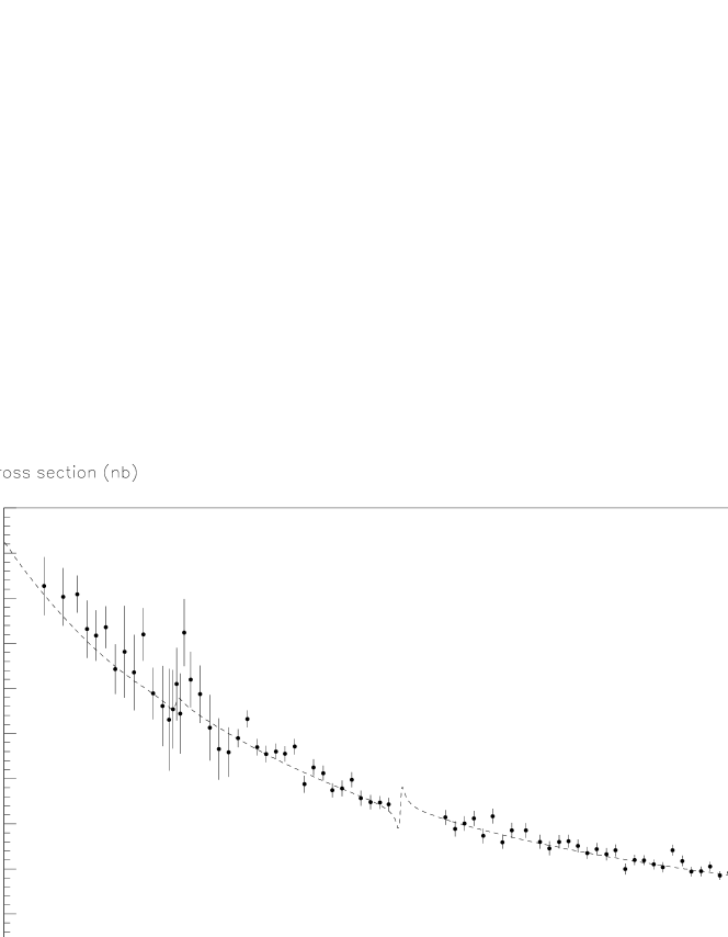
Figure 1: The $e^{+}e^{-}\rightarrow\mu^{+}\mu^{-}$ cross section. The data are shown together with the fit from unitarised VMD2. Other models give similar descriptions.

We find that, disappointingly, the new muon data[46] places no practical constraint on the $\rho$ parameters extracted from $F_{\pi}(q^{2})$. Indeed, the central values for the fit parameters at minimum $\chi^{2}$ are practically the same when fitting only $\pi\pi$ than $\pi\pi+\mu\mu$ data, the errors become slightly larger in the second case (because of the magnitude of the errors in the resonance region with the $\mu\mu$ final state). The errors quoted in Tables 1 and 2 are those obtained when fitting only $\pi\pi$ data up to 1 GeV/c. Thus the single existing data set on the muon final state is not precise enough for our purposes. To improve the situation we require more accurate muon data below $\simeq 1$ GeV/c. This is illustrated by Fig. 1 which shows the muon data together with one of the best fits (namely unitarised VMD2).

Another striking conclusion is that it is generally possible to achieve a very good fit to the pion data whichever model is used, unitarised or not; the single exception to this being non-unitarised VMD2 (which is the usual model for $\rho$ physics). Correspondingly, the significant model dependence of the extracted $\rho$ mass should be noted. We do not give results in case of the non–unitarised WCCWZ model, as in this case the solution converges to $b\simeq 0$ and then coincides with VMD1. We do not present pion data curves for VMD1 and HLS as they show results indistinguishable from Fig. 4 of Ref. [7] which is probably the best possible fit ($\chi^{2}$/dof=61/77). Fig. 2 shows the fit obtained using non-unitarised VMD2; one clearly sees that the model fails to describe the mass region below the $\omega$ mass, while the region from the $\omega$ to the $\phi$ mass is quite correctly reproduced. It is doubtful that taking into account higher mass mesons could cure this problem. On the other hand, Fig. 3 shows the fit obtained using unitarised VMD2 which is of good quality throughout the mass range. Its quality is better than that of M₂ (see Fig. 3 of Ref. [7]) simply because $g_{\rho\gamma}$ (actually, $\epsilon$) is treated here as a free parameter, as it should be.

For the non-unitarised HLS model, the $\rho$ mass and widths appear similar to those obtained in the fit by Bernicha et al. [33], (${m}_{\rho}=757.5\pm 1.5$ MeV and $142.5\pm 3.5$ MeV respectively), which used propagators with constant widths defined in terms of the complex pole locations. The reason can be traced back to the fact that the HLS model mimics quite well a Laurent expansion when there is no mass dependence in the numerator of the $\rho$ contribution as in Eq. (14). The unitarised fits (shown in Table 2), however, all show much higher $\rho$ masses than do the non–unitarised fits.

The values obtained for the widths $\Gamma(\rho\rightarrow\pi^{+}\pi^{-})$ and $\Gamma(\rho\rightarrow e^{+}e^{-})$ and the Orsay phase, $\phi$, are in the expected range. The value for $g_{\rho\gamma}$ is approximately three times that of $g_{\omega\gamma}$ as expected from SU(3) symmetry and ideal mixing [47], and $g_{\rho\pi\pi}^{2}/4\pi$ is always at the expected value (about 3) except for the unitarised WCCWZ model which provides a much smaller value. Moreover, the smallness of the statistical error on $g_{\rho\gamma}$ should be noted,i.e., the uncertainty is essentially all due to model dependence.

The value for $\lambda$ deviates from 1 [see the discussion surrounding Eq. (11)] quite substantially for the standard VMD1 and HLS models, although the unitarised versions return a more standard value. As $\lambda$ is a priori an effective parameter which accounts for higher order effects in the perturbation expansion and/or dynamical left–hand singularities, this is not yet grounds for rejection of the non–unitarised versions of the models. On the other hand, unitarised VMD2 provides, as expected, a value for $\lambda$ close to that found using M₂ in Ref. [7]. We also note that universality ($\epsilon=0$ or $a=2$) is broken significantly in all fits at the level of $\simeq 20\%$. Finally, the effective parameter $b$ introduced in the unitarised WCCWZ model stays relatively small and allows one to obtain a more conventional mass for the $\rho^{0}$ meson[42].

It should be noted that, fixing $\lambda$ to 1 in the non–unitarised versions of VMD1 and HLS, we essentially recover the solutions given in Table 2, as remarked in subsection 2.4; the $\chi^{2}$ value is practically as good. The situation is completely different for VMD2, for which $\lambda$ is found significantly different from 1. As there is no general requirement based on unitarity and analyticity which constrains the value of $\lambda$, nothing can be concluded from this observation. It is however interesting that unitarisation of the VMD1 and HLS models returns $\lambda\simeq 1$; comparing for instance the results for the HLS model given in Table 2 with the corresponding results for model M₃ in Ref. [9], clearly shows that this is a consequence of having released $\Gamma(\rho^{0}\rightarrow e^{+}e^{-})$ in the fits.

As far as one relies only on the statistical quality of fits for the cross section $e^{+}e^{-}\rightarrow\pi^{+}\pi^{-}$, the existing data do not allow one to determine the most suitable way to implement vector meson dominance, except to discard the non–unitarised version of VMD2 which is clearly disfavoured by the data. On the other hand, the possible values for the $\rho^{0}$ mass cover a wide mass range: from 750 MeV to 780 MeV. The single firm conclusion which can be drawn from the above analysis is that, whichever is the VDM parametrisation chosen, unitarised or not, one always observes a small but statistically significant signal of universality violation: $\epsilon\simeq 0.20$ (instead of 0) or $a\simeq 2.4$ (instead of 2).

The question, therefore, remains as to whether it is possible to find other criteria to distinguish between the various ways of building effective Lagrangians involving the vector mesons.

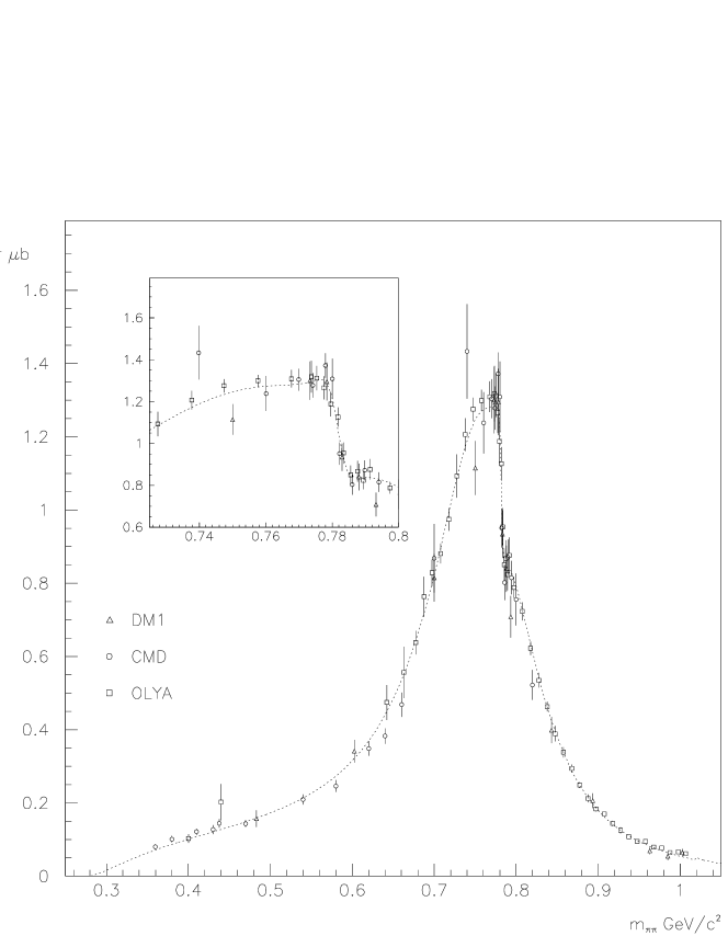
Figure 2: $e^{+}e^{-}\rightarrow\pi^{+}\pi^{-}$ cross section. The data are shown together with the fit curve obtained using VMD2 not unitarised.

Figure 3: $e^{+}e^{-}\rightarrow\pi^{+}\pi^{-}$ cross section. The data are shown together with the fitted curve obtained using unitarised VMD2.

5 Comparison with $\pi\pi$ Phase shift Analysis

Until now, we have focussed on the various ways of implementing the VMD assumption when describing the $e^{+}e^{-}\rightarrow\pi^{+}\pi^{-}$ cross section. As is clear from Section  2, the way to express VMD is not unique. A representative set of possible models has been given in the previous section. We say “representative” in the sense that it is difficult to imagine a class of models very different from the four models studied in both unitarised and non–unitarised forms.

The previous section illustrates that essentially all of the known formulations of VMD are able to provide a quite satisfactory description of the $e^{+}e^{-}$ data. This was a conclusion previously reached in Refs. [7, 9] with models referred to in that work as M₁, M₂ and M₃. As the $e^{+}e^{-}\rightarrow\pi^{+}\pi^{-}$ cross section is not sufficient to differentiate between the various realisations of VMD, comparison with other data and/or information is helpful.

The $e^{+}e^{-}\rightarrow\pi^{+}\pi^{-}$ cross section depends only on $|F_{\pi}(q^{2})|$, i.e., the magnitude of $F_{\pi}$. We have at our disposal a number of models which give equally good fits to this cross-section. Hence we can now examine the ability of each of our versions of the VMD hypothesis to reproduce the $I=l=1$ $\pi\pi$ phase shift data, as we have $\arg{[F_{\pi}(q^{2})]}\equiv\delta_{1}^{1}$, as noticed in Section 2.5.

As previously noted the resonant part of the form factor also contains in general some small isospin zero contributions (e.g., from the $\omega$ and $\phi$). Below 1 GeV, the dominant isospin 1 contribution to strong interactions is the $\rho^{0}$. This was the conclusion previously reached when analysing $\pi\pi$ data [39, 40, 41]. Moreover, it has been shown [44] recently in $\tau$ decay to pion pairs, that the influence of possible higher mass vector isovector mesons ($\rho(1450)$ and $\rho(1700)$) is negligible below $\simeq 1$ GeV. As $\tau$ decays and $e^{+}e^{-}$ annihilation are connected through CVC [48], which has been shown in [49], the conclusion of aleph gives support to neglecting these states in our invariant mass range.

Thus, there is an apparent elasticity of the $P$–wave isovector $\pi\pi$ scattering up to $\simeq 900\div 1000$ MeV. Then , we can limit the relevant resonant contribution to the $I=l=1$ $\pi\pi$ phase shift to the single $\rho$ meson propagator. For VMD2, this means that the opposite of the $\rho^{0}$-propagator phase coincides with the phase $\delta^{1}_{1}$ of the $I=l=1$ $\pi\pi$ partial wave (see Eq. (24)). When dealing with all other models, there is a nonresonant direct $\gamma\pi\pi$ contribution to the pion form factor which also contributes. It is the concern of the present section to check to which extent, the phase of the form factors defined in Section 2 (together with the numerical values obtained from fit to $e^{+}e^{-}\rightarrow\pi^{+}\pi^{-}\;$and listed in Tables 1 and 2) gives an appropriate description of $\delta^{1}_{1}$, as it is determined and/or measured in $\pi\pi$ scattering.

$\pi\pi$ scattering is an important physical process, where the basic concepts of S–matrix theory can be applied with some precision; these basic requirements include unitarity, analyticity and crossing symmetry. In the case of the $\pi\pi$ system, crossing symmetry puts stringent constraints on the partial waves by mean of the Roy equations[50] or dispersion relations. Methods based on these general principles are well known (see, e.g., Ref. [51] and references therein) and have been applied [14] in order to fit and/or reconstruct the $I=l=1$ $\pi\pi$ phase shift $\delta^{1}_{1}$ at low energy (i.e. from threshold up to about 1 GeV). These methods and most of their results are presently encompassed by ChPT [52, 53, 54, 55].

Therefore it is of some interest to compare the phase shifts predicted from the versions of VMD obtained after fitting to the $e^{+}e^{-}\rightarrow\pi^{+}\pi^{-}$ data to the values of $\delta^{1}_{1}$ as tabulated by Ref. [14] (see their Table 1). In this way, it is possible to check the consistency of the information deduced assuming each VMD formulation with the results of Ref. [14] which were derived under completely independent assumptions (namely, unitarity, analyticity and crossing symmetry). One should note that our model errors (those produced by the errors on the fitted parameters) have a small effect on the predicted phase; indeed, the accuracy on the predicted phase is 1.5% at 600 MeV and 0.6% at 800 MeV. From a practical point of view, Ref. [14] does not quote errors. Therefore, we shall unfortunately not be able to express this comparison in terms of statistical quality factors.

Figure 4: $\pi^{+}\pi^{-}$ phase shift $\delta^{1}_{1}$. In both figures, the points are those from Ref. [14]. In (a) curves displayed correspond to non–unitarised models (parameter values taken from Table 1); full line is VMD1, dotted line is HLS and dashed line is VMD2. In (b) the curves displayed correspond to unitarised models (parameter values taken from Table 2); the uppermost curve (dotted) is HLS, the lowest curve (full line) is VMD1; in between, the two curves corresponding to VMD2 and WCCWZ almost superimpose at this scale.

In Fig. 4, we have plotted the curves predicted from our analysis and the phases from Ref. [14]. The non–unitarised versions of VMD1 and HLS can clearly be rejected as failing to support the identification of the $\delta^{1}_{1}$ phase shift with the phase of $F_{\pi}(q^{2})$. Non–unitarised VMD2 looks in better agreement with expectation; however, recall that non–unitarised VMD2 is in poor agreement with $e^{+}e^{-}$ data (see Table 1 above). These remarks are even clearer from Fig. 5, where the difference between the model phases and the data point phase of [14] is plotted. Hence, we conclude that all non–unitarised forms of VMD are disfavored by the data.

Instead, Fig. 4 exhibits remarkably good agreement of all unitarised versions of VMD with the data from Ref. [14] over the full invariant mass range (from the two–pion threshold up to 1 GeV). Taking into account the simplicity of our expressions for $F_{\pi}(q^{2})$, this is already remarkable. The difference between the various predictions for the phase shift and the data of Ref. [14] is presented in Fig. 5(b) for the unitarised models. Clearly, VMD1 fails to describe Froggatt–Petersen phase over the whole invariant mass range, at a finer level of accuracy. Both WCCWZ and VMD2 have a systematic disagreement with the Froggatt–Petersen phase, (it is larger at low energy for WCCWZ than for VMD2). Finally, the HLS model exhibits a quite remarkable agreement with the expected phase up to about 700 MeV, i.e. where the Froggatt–Petersen reconstruction is expected to be highly accurate; in this region the distance to expectation grows slowly, up to only 0.5 degrees near 700 MeV.

Given that the pole location for the $\rho$ in the complex $s$–plane is an input into the phase shift analysis (set at a mass of 767 MeV and a width of 137 MeV and not allowed to vary), the disagreement of about 6 degrees near the $\rho$ mass for the HLS model should not be considered presently as particularly significant and, correspondingly, the fact that the point where the phase goes through $\pi/2$ in Ref. [14] (780 MeV) is close to the mass given by VMD2 (780.4 MeV) should also not be regarded as especially remarkable.

Finally, the relative difficulty for our unitarised models to match the phase above $800\div 900$ MeV (see Figs. 4b and 5b) can also be partly attributed to higher vector mesons which definitely exist [4, 44] and may indeed contribute at a small level in this mass region. However, such additional contributions should not be significant below the $\rho$ peak. One should also notice that the phase shift of [14] is not expected to be as accurate in this invariant mass region as it should be below the $\rho$ mass peak. For all these reasons, the matching of phases in the region $800\div 900$ MeV cannot be considered as constraining as the matching in the region $300\div 600$ MeV.

Figure 5: $\pi^{+}\pi^{-}$ phase shift $\delta^{1}_{1}$. The plots display the difference between the phase shift of Ref. [14] and our phase shifts. In (a) curves displayed correspond to non–unitarised models (parameter values taken from Table 1); full line is VMD1, dotted line is HLS and dashed line is VMD2. In (b) the curves displayed correspond to unitarised models (parameter values taken from Table 2); uppermost curve (dotted) is HLS, lowest curve (full line) is VMD1 and middle curves are (dashed line) VMD2 and (dashed–dotted) WCCWZ .

Figure 6: Function $\sin{\delta^{1}_{1}}/p_{\pi}^{3}$ deduced from $\pi^{+}\pi^{-}$ phase shifts; the function is given in units of $m_{\pi}^{-3}$. The dots correspond to the points of Ref. [14]. Full line is VMD1, dashed line is VMD2, dotted line is HLS (the best description of expected phase) and dashed–dotted is WCCWZ.

Another way to carry on the comparison of the $F_{\pi}(q^{2})$ phases with the Froggatt–Petersen phase shift, is to superimpose the various model predictions for $\sin{\delta^{1}_{1}}/p_{\pi}^{3}$. This function is connected with the isospin 1 $P$–wave scattering length $a_{1}^{1}$ through:

$$a_{1}^{1}=\displaystyle\lim_{q^{2}\rightarrow 4m_{\pi}^{2}}\frac{\sin{\delta^{1}_{1}(q^{2})}}{p_{\pi}^{3}(q^{2})}$$ (30)

and has the characteristic of highly magnifying differences due to the phases in the low energy region (up to, say, 600 MeV). The curves corresponding to the various unitarised models are shown in Fig. 6 together with the points reconstructed using the phase as given in Ref. [14]. Note that erratic behaviour of the values deduced from Ref. [14] at the very beginning of the curve is entirely due to rounding errors only. The general success of the HLS model in matching the low energy $\pi\pi$ phase data is especially remarkable. In terms of angles, in the low energy region the distance to the data points does not exceed a few hundredths of a degree. Instead VMD1 finds 0.02^∘, WCCWZ 0.03^∘ and VMD2 0.06^∘, where the prediction is rather 0.1^∘. In Fig. 7 we present, for all unitarised models, the measured cross section for $e^{+}e^{-}\rightarrow\pi^{+}\pi^{-}$ and the previous fit function behaviours in the low energy region. They are equally as good with the possible exception of VMD2. From this, we conclude that the difference in ability to describe the $\delta^{1}_{1}$ phase shift is due to the existence and the magnitude of a direct $\gamma\pi^{+}\pi^{-}$ coupling within models when fitting $e^{+}e^{-}$ data.

Figure 7: $e^{+}e^{-}\rightarrow\pi^{+}\pi^{-}$ cross section in nb with fits using various unitarised VMD models. Data point and curves are given from threshold to 500 MeV.

The success of the HLS model in reproducing the correct phase values and behaviour is remarkable. This can be partly attributed to the fact that its $\gamma\pi\pi$ coupling is connected with universality violation, while for VMD1, this term is fixed in absolute magnitude to the pion charge. Another reason is connected with the fact that in the HLS model, $g_{\rho\gamma}$ is constant while it is proportional to $q^{2}$ in VMD1 and WCCWZ. This actually produces a too large drop of the resonant contribution to the phase at low invariant mass which is not supported by the data, as it is illustrated in Fig. 6.

On the other hand, the WCCWZ model, while differing from all other models by having a conventional $\rho$ mass and an additional $q^{2}$ dependent term, does not match the phase shift better than VMD1 or VMD2. We may therefore conclude that the extra term in WCCWZ is not consistent with appropriate low-energy behaviour when WCCWZ is constrained to fit the broad energy range ($0.28$ to $1.0$ GeV) rather than near threshold only.

Figs. 4, 6 and 7 demonstrate that, within the class of models considered, a good fit to all experimental data can only be obtained by including an explicit direct $\gamma\pi^{+}\pi^{-}$ coupling term in the model. For the HLS model, the magnitude of this direct coupling is quite well-fixed by data and is approximately $-e/6$ (in contrast to the common form of VMD, VMD2, for which such a term is absent).

Indeed, Fig. 7, clearly shows that the four unitarised models fit practically as well the cross section $e^{+}e^{-}\rightarrow\pi^{+}\pi^{-}\;$in the low energy region. Therefore, their relative ability to account here for the phase $\delta^{1}_{1}$ does not originate from sharp differences in fitting $e^{+}e^{-}\rightarrow\pi^{+}\pi^{-}\;$in the same region. The phase corresponding to the HLS model matches accurately $\delta^{1}_{1}$ [14] from threshold to about 700 MeV, as illustrated by Figs. 4 and 6; this phase coincides with that of $F_{\pi}(q^{2})$. Instead, VMD1 having a $\gamma\pi^{+}\pi^{-}$ coupling of magnitude fixed to $e$, fails to describe accurately this low energy region. VMD2 exhibits a systematic disagreement, which can be traced back to the lack of an explicit $\gamma\pi\pi$ coupling, more important at low energies; it should be remarked that VMD2 is, however, the closest (after HLS) to the data points; this is related to the fact that VMD2 actually corresponds to the HLS model with $a=2$ while the data prefer a slightly different value ($a\simeq 2.4$).

The behaviour of WCCWZ with respect to HLS clearly shows that data considered from threshold to about the $\phi$ mass are more consistent with the existence of a constant nonresonant coupling. Another interesting result is that, from Table 2, it is clear that we can perform the fits with the HLS model fixing $\lambda=1$ without any significant change in the fit quality or in the parameter values. The fact that $\lambda\simeq 1$ is preferred by the data at the fit level is interesting in a number of regards; indeed, $\lambda=1$ is one of the most common ways to parametrise the $\rho$ width; it is also the value obtained for the width for an interaction term in the Lagrangian of the form [27] $\rho^{\mu}(\pi^{+}\partial_{\mu}\pi^{-}-\pi^{-}\partial_{\mu}\pi^{+})$ with constant dressed coupling. We discuss in Section 7, whether a departure of $\lambda$ from 1, even if not significant at the fit level (see Table 2), should be considered. In closing this section we note that no non–unitarised model appropriately reproduces the $\pi\pi$ phase shift [14], and that, among all unitarised models we have examined, only the HLS model of Bando et al. agrees well with the $\pi\pi$ phase shift predictions [14].

6 ChPT and constraints in the near-threshold region

In the preceding sections, we have analysed various realisations of VMD using $e^{+}e^{-}$ data and a $\pi\pi$ phase shift analysis, over the full invariant mass range where data and/or information is available. It is also of interest to examine in detail the consequences of the various VMD models for the magnitude of $F_{\pi}$ in the near threshold region.

From a general perspective (such as that of ChPT, for example), the VMD Lagrangians are rather simple and should not be expected a priori to be able to provide an accurate representation of the full physics of QCD over the whole of the low-energy regime below $1\ {\rm GeV}^{2}$. In particular, it is known that the effects of $\rho$ exchange first show up in the usual Gasser and Leutwyler effective chiral Lagrangian, ${\cal L}_{\rm eff}$, (relevant to processes involving only external $\pi$ legs[53, 56, 57]) as contributions to the fourth order low-energy constants (LEC’s), $L_{k}^{r}$, appearing in ${\cal L}_{\rm eff}$[58]. This means that, very near threshold, other contributions, not generated by $\rho$ exchange, are also, in principle, present in $\pi\pi$ scattering and $F_{\pi}$. The models VMD1, HLS and WCCWZ allow for such a possibility, though in a form much simpler than would necessarily be expected on general principles. The fact that we allow some phenomenological freedom in the treatment of the $s$-dependence of the $\rho$ width, however, means that some of the more complicated $s$-dependence of the non-resonant contribution may be able to be reproduced by a slight adjustment of the parameter $\lambda$. Such a readjustment, of course, has no effect at the $\rho$ peak.

The physical spectral function near threshold in the vector isovector channel, which is measured experimentally in $e^{+}e^{-}\rightarrow\pi^{+}\pi^{-}$ and in $\tau$ decays[44], is very well described near threshold by ChPT[56, 57, 59]. At next-to-leading (two-loop) order in the chiral expansion, the ChPT expression for $F_{\pi}(q^{2})$[60], however, contains two new sixth order LEC’s not constrained by other experimental data, so an improved prediction is not possible at present. However, one can use the form of the two-loop prediction[60],

$$F_{\pi}(q^{2})=1+{\frac{1}{6}}\langle r^{2}\rangle_{V}^{\pi}q^{2}+c_{\pi}q^{4}+f^{U}_{V}(q^{2}/m_{\pi}^{2})+{\cal O}(q^{6}),$$ (31)

(where $f^{U}_{V}$ is a known function, whose explicit form may be found in Ref. [61]) to analyse the near-threshold data and obtain an optimal model-independent fit for the parameters $\langle r^{2}\rangle_{V}^{\pi}$ and $c_{\pi}$. The results are[61]

$$\langle r^{2}\rangle_{V}^{\pi} = 0.431\pm 0.020\pm 0.016\ {\rm fm}^{2}$$

$$c_{\pi} = 3.2\pm 0.5\pm 0.9\ {\rm GeV}^{-4}$$ (32)

where the first error is statistical and the second error theoretical. Note that, although the data analysed is that of the NA7 collaboration[62], the statistical error is roughly a factor of 2 larger than quoted in Ref. [62]. According to the authors of Ref. [61] this larger error reflects the presence of the additional fit parameter, $c_{\pi}$. We will accept the results of the analysis of Ref. [61] since the form of the fit function used, being obtained from ChPT, is the most general one possible, compatible with QCD, to this order in the chiral expansion. As such, the analysis is as model-independent as possible, to this order. Using these results we obtain an experimental value for the threshold value of $F_{\pi}$. In quoting this result below we have added all errors in quadrature. Note that the next-to-leading order contributions appearing in this experimental fit are in agreement with those appearing in the 1-loop ChPT expression for $F_{\pi}(q^{2})$ [57]. This is of interest since, in the case of the one-loop expression, the relevant LEC, $L_{9}^{r}$, is also constrained by other experimental data. Although it is conventional to fix $L_{9}^{r}$ using $\langle r^{2}\rangle_{V}^{\pi}$ as input, fixing it independently through a quantity like the combination $r_{A}/h_{V}$ appearing in the amplitude for the process $\pi^{+}\rightarrow e^{+}\nu_{e}e^{+}e^{-}$ leads to compatible values. As a result, the 1-loop expression for $F_{\pi}$ may be thought of as a prediction.

We now compare the results of the various unitarised models, as fitted to $e^{+}e^{-}$ cross-section data, for $F_{\pi}(4m_{\pi}^{2})$, with the experimental value, obtained as described above

$$\left\{\begin{array}[]{lll}\left[F_{\pi}(4m_{\pi}^{2})\right]_{\rm VMD1}&=&1.174\pm 0.001\\[5.69046pt] \left[F_{\pi}(4m_{\pi}^{2})\right]_{\rm WCCWZ}&=&1.149\pm 0.010\\[5.69046pt] \left[F_{\pi}(4m_{\pi}^{2})\right]_{\rm HLS}&=&1.176\pm 0.001\\[5.69046pt] \left[F_{\pi}(4m_{\pi}^{2})\right]_{\rm VMD2}&=&1.393\pm 0.001\\[5.69046pt] \left[F_{\pi}(4m_{\pi}^{2})\right]_{\rm Expt}&=&1.17\pm 0.01\\[5.69046pt] \end{array}\right.$$ (33)

We see that each of these unitarised VMD models is close to the ChPT result with the exception of VMD2.

In order to quantify our comparison of the low energy phase behaviour we have computed the scattering lengths $a_{1}^{1}$ following from the various unitarised models. For this purpose, Eq. (30) has been used with the corresponding phase of each $F_{\pi}$, following our remarks in Section 2.5; the results are:

$$\left\{\begin{array}[]{lll}a_{1}^{1}(\mbox{VMD1})&=&0.006\pm 0.007\\[5.69046pt] a_{1}^{1}(\mbox{VMD2})&=&0.023\pm 0.002\\[5.69046pt] a_{1}^{1}(\mbox{HLS})&=&0.043\pm 0.003\\[5.69046pt] a_{1}^{1}(\mbox{WCCWZ})&=&0.013\pm 0.002\\[5.69046pt] \end{array}\right.$$ (34)

in units of $m_{\pi}^{-3}$. These values can be compared with experimental results from $K_{e4}$ data [63, 64] using a Roy equation fit ($a_{1}^{1}=0.038\pm 0.002$). The result of Ref. [36] ($a_{1}^{1}=0.10$) disagrees with these results and that treatment violates basic assumptions of ChPT as illustrated in Ref.  [65]. The Current Algebra prediction [66] is $a_{1}^{1}=0.030$ and the ChPT result [54] predicts $a_{1}^{1}=0.037\pm 0.001$ at the two loop order (at ${\cal O}(p^{4})$). A recent preliminary ChPT calculation [67] predicts that the expected value for $a_{1}^{1}$ should increase at order ${\cal O}(p^{6})$ and give a value in the range $0.038\div 0.040$. The range given for this prediction reflects the existing uncertainties in the low energy constants (LEC’s).

The question with the above estimates of the scattering length $a_{1}^{1}$ is twofold : 1) to what extent is the interpolation of each model into the low energy regime and subsequent extraction of $a_{1}^{1}$ meaningful and reliable? 2) is it possible to improve each estimate?

Assuming that the interpolation to low energies is meaningful, which seems legitimate in view of the preceding section (at least for the HLS model), the answer to the “reliability” issue is connected with the fit quality for each case, which is well summarised by the line $\chi^{2}/{\rm dof}(\pi\pi)$ in Table 2. As noted earlier, the best fit quality reached with the existing $e^{+}e^{-}\rightarrow\pi^{+}\pi^{-}$ data [4] corresponds to $\chi^{2}/{\rm dof}=61/77$. This value was already achieved in Refs. [7, 9] with their model M₁; we get it here with the WCCWZ model which is a six parameter fit while M₁ was a five parameter fit (as our present models VMD1, VMD2, HLS). From a statistical point of view, a $\chi^{2}/{\rm dof}=61/76$ is unlikely to be reliably improved and should be considered close to perfection and hence, $a_{1}^{1}(\mbox{WCCWZ})$ cannot be significantly improved. Taking into account the systematic disagreement with the phase of Ref. [14] revealed by Fig. 6, we cannot consider this estimate as reliable.

Unitarised VMD2 gives a very good (even if not perfect) fit to the pion form factor ($\chi^{2}/{\rm dof}=81/77$); however, from Fig. 7, it appears to have some difficulty accommodating all data points as well as the three other VMD models in the low energy region; this can be attributed to the lack of a non–resonant term which is present in the other models.

Finally, VMD1 and the HLS model provide both a near optimum fit ($\chi^{2}/{\rm dof}=65/77$) to the pion form factor, and so cannot be dramatically improved. We thus believe that, numerically, the extrapolation is reliable and cannot be significantly improved. We shall nevertheless examine the consequences of fixing $\lambda=1$ in the next section.

To summarise this section, we can say that among the unitarised versions of the VMD assumption, each of VMD1, WCCWZ and HLS provide a good extrapolation for the magnitude of $F_{\pi}$ all the way down to threshold, while only the HLS model provides additionally a good extrapolation of the phase $\delta^{1}_{1}$. From the discussion above, we can give our extracted value for the scattering length, $a^{1}_{1}=0.043\pm 0.003$, which compares well with the previous measurement [63, 64] (their separation is $1.4\sigma$).

As a consequence of these observations we conclude that, of the models considered, only the unitarised HLS model, with $a\simeq 2.4$, provides a successful representation of $F_{\pi}$ in both magnitude and phase which is valid in the whole region from threshold to the $\phi$ mass.

7 Discussion

The previous analysis of the $e^{+}e^{-}$ data [4] and its comparison with the phase shift $\delta^{1}_{1}$ of Froggatt–Petersen [14], lead us to conclude that the VMD1, VMD2, WCCWZ and HLS unitarised models provide a good description of a very large set of experimental data, as illustrated by Table 2 and by Fig. 4. However, a finer check on the low energy behaviour (see Fig. 6) highly favors the HLS model over all other ways to formulate the VMD assumption. This conclusion is enforced if one includes the known information in the near–threshold region provided by experiments and ChPT (values for $F_{\pi}(4m_{\pi}^{2})$ and $a_{1}^{1}$).

This agreement is reached by allowing the HLS $a$ parameter to slighly depart from its universality value: $a\simeq 2.4$ instead of $a=2$. Relying on this model, we find that universality is violated at a level of 20%. As a direct consequence of this, we observe a non–resonant direct coupling $\gamma\pi^{+}\pi^{-}$, with strength $-0.182\pm 0.008$. The corresponding term in VMD1 is 1 (due to the pion electric charge), while it is 0 for the widely accepted VMD2. Universality violation does not prevent the HLS model fulfilling the constraint $F_{\pi}(0)=1$ in a quite natural way.

Even if the influence of this direct term is the largest near threshold, it contributes a significant improvement up to 1 GeV, because of interferences. This becomes even clearer if one notes that VMD2 is qualitatively equivalent to the HLS model by simply removing the constant term in its expression for $F_{\pi}$ (see section 2). Therefore, we have the first suggestive evidence for a non–zero point–like $\gamma\pi^{+}\pi^{-}$ coupling.

The origin of the shortcomings of the VMD1, VMD2 and WCCWZ models are readily understood. For VMD2, universality violation (required by the data) produces an $F_{\pi}$ which, extrapolated to $q^{2}=0$, has $F_{\pi}(0)-1\equiv\delta>0$. Not surprisingly, near threshold then, the fitted VMD2 model exceeds data by almost exactly $\delta$. For VMD1 and WCCWZ, the problem is the near-threshold phase. In a conventional effective field theory formulation[19], however, the direct pion-photon coupling term in $F_{\pi}$ (unavoidably present) has a non-zero phase via $\pi\pi$ rescattering. The truncated version represented by VMD1 and WCCWZ does not allow for this possibility and the models turn out to be insufficiently flexible to fully compensate for this deficiency by an adjustment of the parameters of the $\rho$ contribution.

An interesting issue is also the observed inequivalence of VMD1 and VMD2. One may argue that this could be a shortcoming due to having neglected mass dependence in the $\rho-\gamma$ coupling produced by loop effects. Following Ref. [27], we have checked that this is not the case, mainly because universality violation is clearly preferred by the data.

Another interesting issue is the value found for $\lambda$ ($1.06\pm 0.08$) in the unitarised HLS model. The departure from 1 is not statistically significant as far as fits of $e^{+}e^{-}$ data alone are concerned and hence the question of whether one can set $\lambda=1$ should be considered. Because of unitarisation (see subsection 2.4), there is no reason why one could not observe departures from 1, which could effectively account for neglected contributions ($t-$ and $u-$channel exchanges, non-resonant strong interaction among pions, higher mass resonances, etc…). The fit value for $\lambda$ shows that these neglected effects are small enough not to spoil the analytical shape generally expected for the $\rho^{0}$ mass–distribution as is obvious from Table 2. However, if all consequences of fixing $\lambda=1$ were acceptable, this will allow us to provide a 4 parameter fit to the pion form factor (the smallest possible set): 3 of these parameters describe the $\rho$ mass and couplings to $\pi^{+}\pi^{-}$ and $e^{+}e^{-}$, and the Orsay phase which is tightly connected with the omega isospin violating contribution.

We have done the fit with the HLS model, fixing $\lambda=1$ in order to get the full set of parameters needed to check accurately the near–threshold results of the preceding section. We have also left free the parameter $A$ which governs the magnitude of Br$(\omega\rightarrow\pi^{+}\pi^{-})$, as it is mainly influenced by $e^{+}e^{-}\rightarrow\pi^{+}\pi^{-}\;$data. As expected, the fit quality is practically unchanged ($\chi^{2}/{\rm dof}=66/77$). We have obtained for $F_{\pi}(4m_{\pi}^{2})=1.177\pm 0.001$, in good agreement with the ChPT expectation and the value reconstructed from other experimental data [61, 62] ($1.17\pm 0.01$). We have also obtained $a^{1}_{1}=0.041\pm 0.003$ using the full phase of $F_{\pi}(q^{2})$, which is in better agreement with the two–loop calculation of [54] ($0.037\pm 0.001$). Moreover, our result is in fairly good agreement with [65] which predicts $a^{1}_{1}=0.040\pm 0.003$, relying on Roy equation techniques. This is consistent with the $\pi\pi$ $P$–wave being nearly purely resonating with only a small background from threshold to 900 MeV. It therefore appears legitimate to fix $\lambda=1$ in our fitting procedure with the unitarised HLS model.

We give as final results those obtained in this last kind of fit with the HLS model [18]:

$$\left\{\begin{array}[]{lll}m_{\rho}(\mbox{MeV})&=&775.1\pm 0.7\\[5.69046pt] \Gamma_{\rho\rightarrow\pi^{+}\pi^{-}}(\mbox{MeV})&=&147.9\pm 1.5\\[5.69046pt] \Gamma_{\rho\rightarrow e^{+}e^{-}}(\mbox{keV})&=&6.3\pm 0.1\\[5.69046pt] \rm{Br}(\omega\rightarrow\pi^{+}\pi^{-})&=&(2.3\pm 0.4)\%\\[5.69046pt] F_{\pi}(4m_{\pi}^{2})&=&1.177\pm 0.001\\[5.69046pt] a_{1}^{1}(m_{\pi}^{-3})&=&0.041\pm 0.003\\[5.69046pt] \phi&=&104.7^{\circ}\pm 4.1^{\circ}\\[5.69046pt] a(\rm{HLS})&=&2.37\pm 0.02\\[5.69046pt] \lambda&=&1~{}~{}(\rm{fixed})\end{array}\right.$$ (35)

Concerning $F_{\pi}(4m_{\pi}^{2})$ the value above is in good agreement with ChPT predictions [57] and the previously quoted experimental value. Our value for $a_{1}^{1}$ compares well with the determination given in [64], which relies on $K_{e4}$ data and the use of Roy equations [50], and with the ChPT calculation of [54] and the Roy equation result [65]. Taking into account the uncertainties on the low energy constants (LEC’s), ChPT at order $p^{6}$ appears consistent [67] with $a_{1}^{1}=0.040$, in good agreement with our extracted value.

A final remark concerning the HLS model is of relevance. As said above, it predicts that the strength of direct $\gamma\pi\pi$ coupling (let us call it provisionally $c$) is tighly connected with universality violation (and then to a small violation of the KSFR relation) by

$$c=\displaystyle 1-\frac{g_{\rho\gamma}g_{\rho\pi\pi}}{m_{\rho}^{2}}$$ (36)

This relation is found to give $c=-0.182\pm 0.008$ when the constraint $c\equiv 1-a/2$ is forced. As a matter of check, we have rerun our fit procedure by decoupling $c$ from $g_{\rho\gamma}$ and $g_{\rho\pi\pi}$. This corresponds exactly to the model M₃ of [9], however leaving free $g_{\rho\gamma}$ as it should. We have, of course, obtained a very good fit ($\chi^{2}/{\rm dof}=66/76$), fixing also $\lambda=1$, which provides $c=-0.171\pm 0.018$, in fairly good agreement with the HLS model result. In other words, the HLS model is able to provide a meaning to the direct coupling $c$ in terms of only the $\rho^{0}$ parameters (see Eq.(36) just above). This (non obvious) correlation was, of course, completely missed in [9], and can be considered as a remarkable success of the HLS model. Finally, the failure of VMD1 and WCCWZ tends also to support the conclusion that $g_{\rho\gamma}$ is more consistent with a constant value, than carrying a $q^{2}$ dependence. Indeed, this $q^{2}$ dependence produces a too strong suppression of the $\rho$ contribution when going down to threshold.

The question is now how to compare the other $\rho^{0}$ parameters given above to the corresponding existing measurements [42]. The main problem with an object as broad as the $\rho^{0}$ meson is that its shape and, correspondingly, its observed parameters are highly influenced by phase space effects and by the production mechanism (creation amplitude). This explains the wide spectrum of values reported in the Review of Particle Physics [42]. Generally, phase space effects are perfectly known and departures from expectations have a physical meaning, as in the decay $\eta^{\prime}\rightarrow\pi^{+}\pi^{-}\gamma$ (see Ref. [9, 68] for instance). In hadronic and in photoproduction experiments, one has to rely on expressions for the production amplitudes $\pi N\rightarrow\rho N$ and $\gamma N\rightarrow\rho N$, which are actually guesses to a large extent; Ref. [34] illustrates the dependence of the $\rho$ mass on several (and all reasonable) guesses for the $\pi N\rightarrow\rho N$ amplitude. In the case of $e^{+}e^{-}$ annihilations, we also work under assumptions which can be discussed (see Ref. [7, 9] for instance) mainly about the transition $\gamma\rightarrow\rho^{0}$ and the possible existence of a constant $\gamma\pi^{+}\pi^{-}$ coupling. One of the original motivations of the present work was indeed to rely on both $e^{+}e^{-}\rightarrow\pi^{+}\pi^{-}$ and $e^{+}e^{-}\rightarrow\mu^{+}\mu^{-}$ data in order to get rid of a possible $\gamma\pi^{+}\pi^{-}$ coupling. We have shown that the single existing data set with $\mu\mu$ final state is not precise enough in the $\rho^{0}$ region in order to achieve this program. However, it happens that the existing information on $\delta_{1}^{1}$, obtained in a completely independent way, allows us to single out the influence of the $\gamma\rightarrow\rho^{0}$ transition and those of the $\gamma\pi^{+}\pi^{-}$ coupling. The quality of the comparison between the phases of the HLS model on the one hand and the data points of Ref. [14] on the other hand shows that these two sources of errors are well controlled.

The fit values obtained for our free parameters and given in Eq. (35) are calibrated by a fit on $e^{+}e^{-}\rightarrow\pi^{+}\pi^{-}\;$data, i.e. they optimise only $|F_{\pi}(q^{2})|$. The expression deduced for $\arg{[F_{\pi}(q^{2})]}$ automatically matches all known information on the phase $\delta^{1}_{1}$ without any further tuning, as illustrated in Sections 5 and 6. Therefore, we conclude that our results in Eq. (35) are little affected by systematic errors due to modelling. The single remaining freedom in defining the $\rho^{0}$ parameters is the definition used for mass and width. What we have quoted corresponds to the most usual Breit–Wigner definition.

Moreover, ChPT predictions [54, 57] near the two–pion threshold allow us to check even more accurately the quality of the information deduced from $e^{+}e^{-}$ data. We can therefore conclude that the HLS model carries information reliable enough to lessen to a large extent the dependence of the $\rho^{0}$ parameters on the production mechanism.

An improvement over the results given in Eq. (35) would require comparison with other independent data and an updating of the Froggatt–Petersen spectrum [14], using more recent data and a more accurate $\rho$ pole position [33]. Moreover, the accuracy of the existing data on $e^{+}e^{-}\rightarrow\pi^{+}\pi^{-}\;$and $e^{+}e^{-}\rightarrow\mu^{+}\mu^{-}\;$is limited by large systematic uncertainties. One can expect a dramatic improvement from the new experiment with the cmd2 detector, now in progress at Novosibirsk, aiming to reach a statistical accuracy of 3% per point and an overall systematic uncertainty better than 1% [69].

Finally, our results suggest a HLS-like model might also prove useful in parametrising hadronic spectral functions measured in $\tau$ decay where, to this point, VMD2-like parametrisations have typically been used [44].

8 Summary and Conclusions

We have studied a variety of vector meson dominance models in both non–unitarised and unitarised forms. They depend on a few parameters (mass of the $\rho$ meson, its coupling constants to $\pi\pi$ and $e^{+}e^{-}$, the shape parameter $\lambda$ and the Orsay phase needed in order to describe the $\rho-\omega$ mixing). We have fitted these to both $e^{+}e^{-}\rightarrow\pi^{+}\pi^{-}$ and $e^{+}e^{-}\rightarrow\mu^{+}\mu^{-}$. In order to study the behaviour of each solution, we have studied how they match the $\pi\pi$ phase shift obtained under general model independent assumptions from threshold up to 1 GeV. We have also examined the value they provide for threshold parameters ($F_{\pi}$ at threshold and the scattering length $a^{1}_{1}$), which can be estimated accurately from ChPT.

This represents the largest set of independent data and cross–checks done so far. It happens that, of the models considered, only the unitarised HLS model is able to account for all examined effects. We also find that the standard value $\lambda=1$, corresponding to a point-like $\rho\pi\pi$ coupling, is well accepted by the data for $\rho$ parametrisation.

Unlike the standard formulation of VMD, fits with this model return a significant non–resonant contribution to the electromagnetic pion form factor. This was found to have a value $\simeq-e/6$. This term is governed by a small universality violation which changes the HLS parameter $a$ from 2 to 2.4. All other models considered, even if they are able to describe $e^{+}e^{-}$ annihilations quite well, are unable to account satisfactorily for the other available information. It should be mentioned that, within the class of models considered, our results tend to favor a constant $g_{\rho\gamma}$ over a $q^{2}$ dependent one.

We give the values for the $\rho^{0}$ mass and for its partial widths to $\pi^{+}\pi^{-}$ and $e^{+}e^{-}$, obtained using the HLS model with $\lambda=1$. This corresponds to describing the resonance mass spectrum through the usual Breit–Wigner expression ($\lambda=1$). We also obtain an estimate of Br$(\omega\rightarrow\pi^{+}\pi^{-})$.

As such, we conclude that, of the models considered, the HLS model with $a\simeq 2.4$ is the most favoured version for implementing the VMD ansatz. Thus, it is interesting to consider whether the success of its predictions for the magnitude and phase of $F_{\pi}(q^{2})$, could be obtained in a way which does not need the assumption that the $\rho$ is a dynamical gauge boson of a hidden local gauge symmetry. Hence, looking for other models able to describe, as successfully as the HLS model, the same large set of data is useful in order to know whether the conceptual motivation for this model should be interpreted as having any underlying significance.

Acknowledgements

We would like to thank J.-L. Basdevant, S. Gardner, M. Knecht, J. Petersen, J. Stern and A.W. Thomas for helpful discussions. This work is supported by the Australian Research Council and the US Department of Energy under grant DE–FG02–96ER40989. It is also supported by Natural Sciences and Engineering Council of Canada.

References

- [1]
- [2] J.E. Augustin et al., Phys. Rev. Lett. 30 (1973) 462.
- [3] D. Benaksas et al., Phys. Lett. B39 (1972) 289.
- [4] L.M. Barkov et al., Nucl. Phys. B256 (1985) 365.
- [5] L. M. Kurdadze et al., Sov. Journ. of Nucl. Phys. 35 (1982) 201; I.B. Vasserman et al., Phys. Lett. B99 (1981) 62.
- [6] H.B. O’Connell, B.C. Pearce, A.W. Thomas and A.G. Williams, Prog. Part. Nucl. Phys. 39 (1997) 201.
- [7] M. Benayoun et al., Zeit. Phys. C58 (1993) 31.
- [8] A. Sirlin, Phys. Rev. Lett. 67 (1991) 2127; R.G. Stuart, Phys. Rev. Lett. 70 (1993) 3193, Phys. Rev. D52 (1995) 1655.
- [9] M. Benayoun et al., Zeit. Phys. C65 (1995) 399.
- [10] M. Chanowitz, Phys. Rev. Lett. 35 (1975) 977.
- [11] M. Chanowitz, Phys. Rev. Lett. 44 (1980) 59.
- [12] J. Wess and B. Zumino, Phys. Lett. B37 (1971) 95.
- [13] W. Weise, Phys. Rep. 13 (1974) 53.
- [14] C.D. Froggatt and J.L. Petersen, Nucl. Phys. B129 (1977) 89.
- [15] B.L. Roberts, Zeit. Phys. C56 (1992) S101; V.W. Hughes, Frontiers of High Energy Spin Physics, ed. T. Hasegawa et al. pp. 717-722 (Universal Academy Press, Tokyo, 1992).
- [16] T. Kinoshita, B. Nižić and Y. Okamoto, Phys. Rev. D31 (1985) 2108; S. Eidelman and F. Jegerlehner, Zeit. Phys. C67 (1995) 585; D.H. Brown and W.A. Worstell, Phys. Rev. D54 (1996) 3237; B. Krause, Phys. Lett. B390 (1997) 392.
- [17] C.D. Roberts, Nucl. Phys. A605 (1996) 475.
- [18] M. Bando,T. Kugo, S. Uehara, K. Yamawaki and T. Yanagida, Phys. Rev. Lett. 54 (1985) 1215.
- [19] S. Weinberg, Phys. Rev. 166 (1968) 1568; S. Coleman, J. Wess and B. Zumino, Phys. Rev. 177 (1969) 2239; C. Callan, S. Coleman, J. Wess and B. Zumino, ibid. 2247.
- [20] M. Birse, Zeit. Phys. A355 (1996) 231.
- [21] K. Mitchell, P. Tandy, C. Roberts and R. Cahill, Phys. Lett. B335 (1994) 282; M.R. Frank and P.C. Tandy, Phys. Rev.C49 (1994) 478; M.R. Frank, Phys. Rev. C51 (1995) 987.
- [22] H.B. O’Connell, A.G. Williams, M. Bracco and G. Krein, Phys. Lett. B370 (1996) 12.
- [23] H.B. O’Connell, B.C. Pearce, A.W. Thomas and A.G. Williams, Phys. Lett. B354 (1995) 14.
- [24] K. Maltman, H.B. O’Connell and A.G. Williams, Phys. Lett. B376 (1996) 19.
- [25] J.P. Perez-y-Jorba and F.M. Renard, Phys. Rep. 31 (1977) 1.
- [26] J.J. Sakurai, Currents and Mesons, University of Chicago Press, 1969.
- [27] F. Klingl, N. Kaiser and W. Weise, Zeit. Phys. A356 (1996) 193.
- [28] J.J. Sakurai, Ann. Phys. 11 (1960) 1.
- [29] N.M. Kroll, T.D. Lee and B. Zumino, Phys. Rev. 157 (1967) 1376.
- [30] C.J. Burden, J. Praschifka and C.D. Roberts, Phys. Rev. D46 (1992) 2695.
- [31] G. Gournaris and J. Sakurai, Phys. Rev. Lett. 21 (1968) 244.
- [32] R. Eden et al., The Analytic S Matrix, Cambridge University Press, 1966.
- [33] A. Bernicha, J. Pestieau and G. Lopez Castro, Phys. Rev. D50 (1994) 4454.
- [34] J. Pisut and M. Roos, Nucl. Phys. B6 (1968) 325.
- [35] M. Hashimoto, Phys. Rev. D54 (1996) 5611; Phys. Lett. B381 (1996) 465.
- [36] B.V. Geshkenbein, Zeit. Phys. C45 (1989) 351.
- [37] P.L. Chung et al., Phys. Lett. B205 (1988) 545.
- [38] G.F. Chew, S–Matrix Theory of Strong Interactions, W.A. Benjamin, New York, 1962.
- [39] P. Estabrooks and A.D. Martin, Nucl. Phys. B79 (1974) 301.
- [40] J.P. Baton et al., Phys. Lett. B33 (1970) 525.
- [41] S.D. Protopescu et al., Phys. Rev. D7 (1973) 1279.
- [42] R.M. Barnett et al., Review of Particle Physics, Phys. Rev. D54 (1996) 1.
- [43] S. Gasiorowicz, “Elementary Particle Physics”, John Wiley and Sons, New York, 1966, Chapter 26 (“Form Factors”).
- [44] R. Barate et al., Zeit. Phys. C76 (1997) 15.
- [45] S. Iwao and M. Shako, Lett. Nuovo Cim. 9 (1974) 693.
- [46] L.M. Kurdadze et al., Sov. Journ. of Nucl. Phys. 40 (1984) 286; B. Shwartz, “Investigation of the reaction at Energies up to 1400 MeV”, PhD Thesis, Novosibirsk, 1983.
- [47] G. Dillon and G. Morpurgo, Zeit. Phys. C64 (1994) 467.
- [48] Y.S. Tsai, Phys. Rev. D4 (1971) 2821.
- [49] F.J. Gilman and S.H. Rhie, Phys. Rev. D31 (1985) 1066; J.H. Kühn and A. Santamaria, Zeit. Phys. C48 (1990) 445; S.I. Eidelman and V.N. Ivanchenko, Phys. Lett. B257 (1991) 437.
- [50] S.M. Roy, Phys. Lett. B36 (1971) 353.
- [51] J.L. Basdevant, C.D. Froggatt and J.L. Petersen, Nucl. Phys. B72 (1974) 413.
- [52] J. Gasser and H. Leutwyler, Phys. Lett. B125 (1983) 325.
- [53] J. Gasser and H. Leutwyler, Ann. Phys. (NY) 158 (1984) 142.
- [54] M. Knecht et al. Nucl. Phys. B457(1995) 513.
- [55] M. Knecht et al., Nucl. Phys. B471 (1996) 445.
- [56] J. Gasser and H. Leutwyler, Nucl. Phys. B250 (1985) 465.
- [57] J. Gasser and H. Leutwyler, Nucl. Phys. B250 (1985) 517.
- [58] G. Ecker, J. Gasser, A. Pich and E. de Rafael, Nucl. Phys. B321 (1989) 311.
- [59] E. Golowich and J. Kambor, Nucl. Phys. B447 (1995) 373.
- [60] J. Gasser and U.-G. Meissner, Nucl. Phys. B357 (1991) 90.
- [61] G. Colangelo, M. Finkemeier and R. Urech, Phys. Rev. D54 (1996) 4403.
- [62] S. R. Amendolia et al., Nucl. Phys. B277 (1986) 168.
- [63] M.M. Nagels et al., Nucl. Phys. B147 (1979) 189.
- [64] L. Rosselet et al., Phys. Rev. D15 (1977) 574.
- [65] J.L. Basdevant et al., Nucl. Phys. B98 (1975) 285.
- [66] S. Weinberg, Phys. Rev. Lett. 17 (1966) 616.
- [67] J. Bijnens et al., hep-ph/9707291, July 1997.
- [68] A. Abele et al., Phys. Lett. B402 (1997) 195.
- [69] B.I. Khazin, Proceedings of the XXVIIth International Conference on High Energy Physics, 1994, Glasgow, Scotland UK, Vol II, p.419.