SNUTP 97-105

Radiative Muon Capture
in Heavy Baryon Chiral Perturbation Theory
Shung-ichi Ando and Dong-Pil Min
Department of Physics and Center for Theoretical Physics,
Seoul National University, Seoul 151-742, Korea

The radiative muon capture(RMC) on a proton is analyzed by means of heavy baryon chiral perturbation theory. The emitted photon energy spectrum is calculated and compared with the experimental data by taking the spin sum on the muonic atom states. We find that one-loop order corrections to the tree order amplitude modify the photon spectrum by less than five percent. This calculation supports that the theory is under a quantitative control as far as the chiral perturbation expansion is concerned and indicates that the discrepancy between the pseudo-scalar coupling constant required by the RMC experiment and the one deduced from ordinary muon capture, the value of which is also supported by chiral perturbation calculations, will remain unexplained from the theoretical side.

Key wards; $\mu^{-}+p\rightarrow\nu n\gamma$, heavy baryon chiral perturbation theory, pseoudo-scalar coupling

PACS: 24.40.-s, 12.39.Fe, 13.60.-r

The induced pseudo-scalar coupling constant $g_{P}$ was determined from the ordinary muon capture (OMC) reaction on a proton $(p+\mu\rightarrow n+\nu)$[1] to be $g_{P}=8.7\pm 1.9$. Despite its large error bar, this value is clearly consistent with the theoretical prediction by Bernard et al. [2] using heavy baryon chiral perturbation theory (HBChPT), $g_{P}(q^{2}=-0.88m_{\mu}^{2})=8.44\pm 0.16$. This is also comparable to the value that Fearing et al. [3] evaluated by means of HBChPT in their work on OMC, $g_{P}(-0.88m_{\mu}^{2})=8.21\pm 0.09$. Together with the PCAC prediction $g_{P}^{PCAC}(-0.88m_{\mu}^{2})=8.42$, all theoretical investigations agree with the experimental result on OMC. However, the momentum transfer involved in OMC is far from the pion pole, $q^{2}=m_{\pi}^{2}$, where the pseudo-scalar coupling should play important role in the reaction amplitude, accounting for the large error bar.

Since RMC involves a momentum transfer closer to the pion mass, it is considered to be more suitable to measure the constant $g_{P}$ and lower the error bar. For this purpose, the photon energy spectrum from the radiative muon capture (RMC) ($p+\mu\rightarrow n+\nu+\gamma$) has been measured in TRIUMF [4] and compared to the model prediction of [5]. Surprisingly, the experimentally detected photon spectrum could be explained only if the pseudo-scalar coupling constant is enhanced in the model by a factor of 1.5 relative to the value given by PCAC [6] or that determined in OMC. A calculation to tree order, recently reported by Meissner et al.[7], further confirms this discrepancy.

The purpose of this paper is to see whether or not this discrepancy can be eliminated by higher order terms in the treatment of the strong interaction sector of the process. It is natural to ask whether any important Feynman diagrams have been ignored in the phenomenological model, in particular in light of the direct chiral perturbation calculation of the pseudo-scalar coupling constant by Bernard et al. [2] which agrees with the PCAC prediction. Experiments are currently being planned[8] to increase the precision.

In this work, we shall calculate the RMC amplitude and the photon energy spectrum using the HBChPT up to the next-to-next to the leading order (${\rm N^{2}LO}$), that is, to one-loop order. We shall also investigate the photon energy spectrum by taking various ansätze on the spin states of the muonic atom.

Heavy baryon chiral perturbation theory(HBChPT)[9] provides a systematic way of making, in the presence of nucleons, a chiral perturbation expansion in powers of $Q/\Lambda_{\chi}$, where $Q$ is a typical momentum scale and/or the pion mass and $\Lambda_{\chi}$ is the chiral symmetry scale, $\Lambda_{\chi}\sim 1{\rm GeV}$. Since the momentum transfer involved in RMC can be of the order of the muon mass, $m_{\mu}\sim 0.1\Lambda_{\chi}$, the chiral expansion is expected to converge sufficiently rapidly.

The Feynman graphs contributing to RMC can be classified into two classes as shown in Fig. 1:

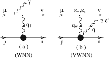
Figure 1: Diagrams for three and four point Greens functions.

(a) the first corresponds to those graphs where the photon line is attached to the lepton, therefore, leaving the nucleon line to form the 3-point vertex of $WNN$ (weak current-nucleon-nucleon), (b) the second corresponds to the graphs where the photon is attached to the nucleon line and the vertex with the exchanged pion coupled to the weak boson, which is schematically a 4-point vertex of $VWNN$ (electro-magnetic current-weak current-nucleon-nucleon). Indeed, those two vertex graphs shown as blobs in Fig. 1 can be expressed in terms of Green’s functions as follows,

$$J^{f}_{\beta}(q_{J},k) = -\chi^{\dagger}_{n}S_{N}^{-1}(k^{\prime})\prod^{3}_{i=1}\int\frac{d^{4}x_{i}}{(2\pi)^{4}}{\rm exp}\left[-i(q_{J}\cdot x_{1}-k^{\prime}\cdot x_{2}+k\cdot x_{3})\right]$$ (1)

$$\times\langle 0|T\ W^{f}_{\beta}(x_{1})N(x_{2})\bar{N}(x_{3})|0\rangle S_{N}^{-1}(k)\chi_{p},$$

$$M^{ef}_{\alpha\beta}(q,q_{W},k) = -i\chi^{\dagger}_{n}S_{N}^{-1}(k^{\prime})\prod^{4}_{i=1}\int\frac{d^{4}x_{i}}{(2\pi)^{4}}{\rm exp}\left[-i(-q\cdot x_{1}+q_{W}\cdot x_{2}-k^{\prime}\cdot x_{3}+k\cdot x_{4})\right]$$ (2)

$$\times\langle 0|T\ V^{e}_{\alpha}(x_{1})W^{f}_{\beta}(x_{2})N(x_{3})\bar{N}(x_{4})|0\rangle S_{N}^{-1}(k)\chi_{p},$$

where $e$,$f$ and $\alpha$,$\beta$ are the iso-spin and Lorentz indices, respectively, and $T$ stands for the time ordering on the currents and fields appearing on its right. Note that the vacuum expectation value in the above equations is the Green’s function. The four-momenta carried by proton, neutron, neutrino, muon are denoted by the particle symbols, $p$, $n$, $\nu$, $\mu$, respectively, whereas the four-momentum of the photon by $q$. The momentum transfers described in Fig. 1 can be written as $q_{W}=\mu-\nu$ and $q_{J}=q_{W}-q$. Here $\chi_{p}$ ($\chi_{n}$) is a two-component spinor of the proton (neutron) with the normalization condition $\chi^{\dagger}\chi=E+m_{N}$, and $S_{N}^{-1}(k)$ is the inverse of the heavy nucleon propagator to be derived below. In the above, $k$ ($k^{\prime}$) denotes the residual momentum of the proton (neutron) so that

$$p^{\mu} = m_{N}v^{\mu}+k^{\mu},$$ (3)

$$n^{\mu} = m_{N}v^{\mu}+k^{\prime\mu},$$ (4)

with the velocity four-vector $v_{\mu}=(1,\vec{0})$. $m_{N}$ is the physical nucleon mass. The heavy nucleon field $N$ is defined from the nucleon field $\Psi_{N}$ as

$$N=e^{im_{N}v\cdot x}P_{+}\Psi_{N},$$ (5)

where $P_{+}$ is the projection operator defined by $P_{+}=\frac{1}{2}(1+v\cdot\gamma)$.

The Green’s functions in Eqs.(1) and (2) are to be obtained from the effective chiral lagrangian with nucleons and pions, the expression of which reads

$${\cal L}={\cal L}_{0}+{\cal L}_{1}+{\cal L}_{2}+\cdots,$$ (6)

where ${\cal L}_{0}$ is the leading order lagrangian given in [10] and ${\cal L}_{1}$ is of the $1/m_{N}$ correction (NLO) which will be specified below. ${\cal L}_{2}$ is the next-to-next leading order (${\rm N^{2}LO}$) effective lagrangian. The ellipses stand for higher order lagrangians irrelevant for our calculation. ${\cal L}_{1}$ reads[10]

$${\cal L}_{1} = \frac{1}{2m_{N}}\bar{N}\left[-D^{2}+(v\cdot D)^{2}+2g_{A}\{v\cdot\Delta,S\cdot D\}\right.$$ (7)

$$+b_{1}{\rm Tr}(\chi_{+})+b_{2}(\chi_{+}-\frac{1}{2}{\rm Tr}(\chi_{+}))+(g_{A}^{2}+b_{3})(v\cdot\Delta)^{2}+b_{4}\Delta\cdot\Delta$$

$$\left.-[S^{\mu},S^{\nu}]\left(2(1+b_{5})\Delta_{\mu}\Delta_{\nu}+i(1+b_{6})f^{+}_{\mu\nu}+i(1+b_{7})v^{S}_{\mu\nu}\right)\right]N,$$

where we have adopted the notations $D_{\mu}$, $\Delta_{\mu}$, $\chi_{+}$, $f^{+}_{\mu\nu}$ and $v^{S}_{\mu\nu}$ as defined in Ref.[10], except for an additional multiplication factor 1/2 for our $f^{+}_{\mu\nu}$. $g_{A}$ is the axial-vector current coupling constant, and $b_{i}$ are the low energy constants that cannot be fixed by the theory, but will be determined from experiments. We should note that for RMC, only the two constants $b_{6}$ and $b_{7}$ are relevant. They are determined from the anomalous magnetic moments of nucleon as $b_{6}=\kappa_{V}=3.71$ , $b_{7}=\kappa_{S}=-0.12$, where $\kappa_{V}$ and $\kappa_{S}$ are the iso-vector and iso-scalar anomalous magnetic moment, respectively. The ${\rm N^{2}LO}$ lagrangian ${\cal L}_{2}$ containing low energy constants and an anomaly term reads

$${\cal L}_{2}=i\alpha_{9}^{(2)}{\rm Tr}(L_{\mu\nu}\nabla^{\mu}U\nabla^{\nu}U^{\dagger}+R_{\mu\nu}\nabla^{\nu}U^{\dagger}\nabla^{\nu}U)+\alpha_{10}^{(2)}{\rm Tr}(L_{\mu\nu}UR_{\mu\nu}U^{\dagger})+{\cal L}_{WZ}$$ (8)

$$+\frac{1}{4m_{N}^{2}}\bar{N}\left[iD^{\alpha}v\cdot DD_{\alpha}-2i[S^{\alpha},S^{\beta}]D_{\alpha}v\cdot DD_{\beta}+ig_{A}[2D\cdot\Delta S\cdot D-2D^{\alpha}S\cdot\Delta D_{\alpha}\right.$$

$$+2S\cdot D\Delta\cdot D+2v\cdot DS\cdot\Delta v\cdot D-2\{S\cdot D,\{v\cdot D,v\cdot\Delta\}\}-i\epsilon^{abcd}D_{a}\Delta_{b}D_{c}v_{d}]$$

$$+i[-v^{\alpha}D^{\beta}+v^{\beta}D^{\alpha}-2v^{\alpha}[S^{\beta},S\cdot D]+2v^{\beta}[S^{\alpha},S\cdot D]+2g_{A}(v^{\alpha}S^{\beta}-v^{\beta}S^{\alpha})v\cdot\Delta]B_{\alpha\beta}$$

$$\left.+iB_{\alpha\beta}[v^{\alpha}D^{\beta}-v^{\beta}D^{\alpha}-2v^{\alpha}[S^{\beta},S\cdot D]+2v^{\beta}[S^{\alpha},S\cdot D]-2g_{A}(v^{\alpha}S^{\beta}-v^{\beta}S^{\alpha})v\cdot\Delta]\right]N$$

$$+\frac{1}{(4\pi f_{\pi})^{2}}\bar{N}\left[c_{3}v^{\alpha}[D^{\beta},f_{\alpha\beta}^{+}]+c_{4}[S^{\alpha},S^{\beta}]\{v\cdot D,f_{\alpha\beta}^{+}\}+c_{8}g_{A}v^{\alpha}S^{\beta}[v\cdot\Delta,f_{\alpha\beta}^{+}]\right.$$

$$\left.+c_{12}[S^{\alpha},S^{\beta}]\{v\cdot D,v_{\alpha,\beta}^{S}\}+c_{13}g_{A}S^{\alpha}[D_{\alpha},f_{\alpha\beta}^{-}]+ic_{14}g_{A}S^{\alpha}[D_{\alpha},\chi_{-}]\right]N,$$

with

$$B_{\alpha\beta}=i\frac{b_{6}}{2}f^{+}_{\alpha\beta}+i\frac{b_{7}}{2}v^{S}_{\alpha\beta}$$ (9)

where ${\cal L}_{WZ}$ is the Wess-Zumino lagrangian[14]. Note that we have eight low-energy constants, among which seven of them are needed for this work: $\alpha_{9}^{(2)}+\alpha_{10}^{(2)}=1.43\times 10^{-3}$ determined from a rare pion process[11], $c_{3}=5.34$ ($c_{13}=2.37$) from the iso-vector vector (axial-vector) radius, $c_{14}=-1.37$ from the Goldberger-Treiman discrepancy[2, 3], $c_{8}=-3.27$ from the $\Delta$ contribution to $E^{(-)}_{0+}$[12], $c_{4}=-22.27$ and $c_{12}=-0.79$ from the $\rho$, $\omega$ and $\Delta$ contributions to $P^{0,-}_{3}$[13]. In short, the constants are completely determined for calculating up to the ${\rm N^{2}LO}$ order in chiral perturbation expansion.

We are now in a position to calculate the relevant Feynman graphs. The chiral power counting rule for A-nucleon processes is that for a Feynman graph with $V_{i}$ vertices of type $i$, $L$ loops, and $C$ separately connected pieces, the power index of $Q$ is given by $\eta=4-A-2C+2L+\sum_{i}V_{i}\Delta_{i}$ with $\Delta_{i}=d_{i}+n_{i}/2-2$, where $n_{i}$ is the number of nucleon lines and $d_{i}$ is the number of derivatives or powers of $m_{\pi}$ at the $i-$type vertex. In the presence of an external gauge field, $\Delta_{i}$ is constrained by chiral symmetry to be $\Delta_{i}\geq-1$[15]. Thus the leading order of matrix elements $J$ is $O(1)$ and that of $M$ is $O(Q^{-1})$. However, the leading order amplitudes of Fig. 1(a) and Fig. 1(b) are of the same chiral order, because the muon propagator in Fig. 1(a) is of order $Q^{-1}$ since it carries the photon momentum in the denominator.

Now we split the weak-current into the $V-A$ form so that the $J$ and $M$ can be written

$$J = J_{V}-J_{A},$$ (10)

$$M = M_{V}-M_{A},$$ (11)

The most general forms of $J$ turn out to be, (with $v_{\mu}=(1,\vec{0})$)

$$\left.\begin{array}[]{c}J^{0}_{V}(q_{J},k=0)=f_{1}^{V},\ \ \vec{J}_{V}(q_{J},k=0)=i\,\vec{\sigma}\times\hat{q}_{J}f_{2}^{V}+\hat{q}_{J}f_{3}^{V},\\ J^{0}_{A}(q_{J},k=0)=\vec{\sigma}\cdot\hat{q}_{J}f_{3}^{A},\ \ \vec{J}_{A}(q_{J},k=0)=\vec{\sigma}f_{1}^{A}+\hat{q}_{J}\vec{\sigma}\cdot\hat{q}_{J}f_{2}^{A},\end{array}\right.$$ (12)

where as is done in what follows, the initial and final state nucleon spinors are omitted. $f^{V}_{i}$ and $f^{A}_{i}$ denote the nucleon vector and axial-vector form factors, respectively. They read as, up to ${\rm N^{2}LO}$,

$$f_{1}^{V} = 1+\frac{c_{3}}{(4\pi f_{\pi})^{2}}q_{J}^{2}-\frac{1+17g_{A}^{2}}{18(4\pi f_{\pi})^{2}}q_{J}^{2}+\frac{1}{(4\pi f_{\pi})^{2}}\left[\frac{2}{3}(1+2g_{A}^{2})m_{\pi}^{2}-\frac{1+5g_{A}^{2}}{6}q_{J}^{2}\right]f_{0}(q_{J})$$ (13)

$$+\frac{1}{4m_{N}^{2}}(-\frac{3}{2}+\kappa_{V})q_{J}^{2},$$

$$f_{2}^{V} = \frac{1}{2m_{N}}(1+\kappa_{V})|\vec{q}_{J}|+\frac{g_{A}^{2}}{64\pi f_{\pi}^{2}m_{\pi}}q_{J}^{2}|\vec{q}_{J}|+\left(\frac{g_{A}}{4\pi f_{\pi}}\right)^{2}\frac{\pi(4m_{\pi}^{2}-q_{J}^{2})}{4m_{\pi}}m_{0}(\vec{q}_{J})|\vec{q}_{J}|,$$ (14)

$$f_{3}^{V} = \frac{1}{2m_{N}}|\vec{q}_{J}|,$$ (15)

$$f_{1}^{A} = g_{A}\left[1+\left(\frac{c_{13}}{(4\pi f_{\pi})^{2}}-\frac{1}{8m_{N}^{2}}\right)q_{J}^{2}\right],$$ (16)

$$f_{2}^{A} = g_{A}\left[\frac{c_{13}}{(4\pi f_{\pi})^{2}}+\Delta_{\pi}(q_{J})\left(1-\frac{2m_{\pi}^{2}c_{14}}{(4\pi f_{\pi})^{2}}+\frac{1}{8m_{N}^{2}}q_{J}^{2}\right)\right]|\vec{q}_{J}|^{2},$$ (17)

$$f_{3}^{A} = \frac{g_{A}}{2m_{N}}[1+\Delta_{\pi}(q_{J})q_{J}^{2}]|\vec{q}_{J}|,$$ (18)

with

$$f_{0}(q) = \int^{1}_{0}dx{\rm ln}[1-x(1-x)\frac{q^{2}}{m_{\pi}^{2}}],$$ (19)

$$m_{0}(\vec{q}) = 1-\int^{1}_{0}dx\frac{1}{\sqrt{1+x(1-x)\vec{q}^{2}/m_{\pi}^{2}}}.$$ (20)

The common factor $2m_{N}$ is omitted in the above equations, and $g_{A}=1.25$. The convergence of the form factors $f_{i}^{V(A)}$ is found to be quite good as is discussed in Ref.[2, 3, 10].

Under the Coulomb gauge, the renormalized inverse propagators for our calculation can be written simply as

$$S_{N}^{-1}(k) = v\cdot k+\frac{1}{2m_{N}}[k^{2}-v\cdot k^{2}],$$ (21)

$$\Delta_{\pi}^{-1}(q) = q^{2}-m_{\pi}^{2}.$$ (22)

We choose the coordinate frame such that the neutrino lies in the $z$-direction and the photon in the $x$-$z$ plane, respectively, i.e., $\hat{\nu}=(0,0,1)$ and $\hat{q}=({\rm sin}\theta,0,{\rm cos}\theta)$, where $\theta$ is the angle between the neutrino and the photon. Then we can decompose $M$ into so-called reduced amplitudes for each muon spin states lying along $z$-axis, $m_{s}=\pm 1/2$ [16],

$$M = -\vec{\epsilon}_{T}\cdot\vec{M}_{T}\ \delta_{m_{s},1/2}+\epsilon_{L,3}\ M_{L}\ \delta_{m_{s},-1/2},$$ (23)

where $\epsilon^{\beta}_{T}=\epsilon^{\beta}_{(1/2)}$ and $\epsilon^{\beta}_{L}=\epsilon^{\beta}_{(-1/2)}$ with $\epsilon^{\beta}_{(m_{s})}\equiv\bar{u}_{\nu}\gamma_{5}(1-\gamma^{\beta})u_{\mu}^{(m_{s})}$.

Then generally one can decompose them into different spin operators as specified in Tables 1 and 2,

$$-\vec{\epsilon}_{T}\cdot\vec{M}_{A,T}=\sum_{i=1}^{6}A_{i}{\cal O}_{a,i},\ \ \ M_{A,L}=\sum_{i=7}^{10}A_{i}{\cal O}_{a,i},$$ (24)

$$-\vec{\epsilon}_{T}\cdot\vec{M}_{V,T}=\sum_{i=1}^{9}B_{i}{\cal O}_{b,i},\ \ \ M_{V,L}=\sum_{i=10}^{13}B_{i}{\cal O}_{b,i},$$ (25)

where ${\cal O}_{a,i}$ and $A_{i}$ (${\cal O}_{b,i}$ and $B_{i}$) are operators and corresponding form factors, respectively. The Ward-Takahashi (WT) identity was found to be quite useful in reducing redundancy in the form factors. Summation runs over all possible effective operators.

$i$	${\cal O}_{b,i}$	$A_{i}^{LO}$	$A_{i}^{NLO}$	$|m_{\mu}A_{i}^{loop}|_{max}$
$1$	$i\hat{q}\cdot\vec{\epsilon}^{*}\times\vec{\epsilon}_{T}$	$0$	$-\frac{g_{A}}{2m_{N}}(1+\kappa_{V})$	$0.030$
$2$	$\vec{\sigma}\cdot\vec{\epsilon}^{*}\ \vec{\epsilon}_{T}\cdot\hat{q}$	$0$	$-\frac{g_{A}}{2m_{N}}(1+\kappa_{S})$	$0.207$
$3$	$\vec{\sigma}\cdot\hat{q}\ \vec{\epsilon}^{*}\cdot\vec{\epsilon}_{T}$	$-g_{A}\Delta_{\pi}(q_{J})E_{\gamma}$	$\frac{g_{A}}{2m_{N}}(1+\kappa_{S})$	$0.232$
$4$	$\vec{\sigma}\cdot\hat{q}_{W}\ \vec{\epsilon}^{*}\cdot\vec{\epsilon}_{T}$	$g_{A}\Delta_{\pi}(q_{J})E_{\nu}$	$0$	$0.001$
$5$	$\vec{\sigma}\cdot\hat{q}\ \vec{\epsilon}^{*}\cdot\hat{q}_{W}\ \vec{\epsilon}_{T}\cdot\hat{q}$	$0$	$0$	$0.001$
$6$	$\vec{\sigma}\cdot\hat{q}_{W}\ \vec{\epsilon}^{*}\cdot\hat{q}_{W}\ \vec{\epsilon}_{T}\cdot\hat{q}$	$0$	$0$	$0.001$
$7$	$i\vec{\epsilon}^{*}\cdot\hat{q}\times\hat{q}_{W}$	$0$	$\frac{-g_{A}}{2m_{N}}(1+\kappa_{V})$	$0.033$
			$\times(1+\Delta_{\pi}(q_{W})m_{\mu}E_{\nu})$
$8$	$\vec{\sigma}\cdot\vec{\epsilon}^{*}$	$-g_{A}\Delta_{\pi}(q_{W})m_{\mu}$	$\frac{-g_{A}}{2m_{N}}\left[(1+\kappa_{S})\right.$	$0.219$
			$\times(1+\Delta_{\pi}(q_{W})m_{\mu}E_{\nu})y$
			$\left.-(1-\Delta_{\pi}(q_{W})m_{\mu}E_{\gamma})\right]$
$9$	$\vec{\sigma}\cdot\hat{q}\ \vec{\epsilon}^{*}\cdot\hat{q}_{W}$	$g_{A}\Delta_{\pi}(q_{J})E_{\gamma}(1+$	$\frac{-g_{A}}{2m_{N}}(1+\kappa_{S})$	$0.184$
		$2\Delta_{\pi}(q_{W})m_{\mu}E_{\nu})$	$\times(1+\Delta_{\pi}(q_{J})m_{\mu}E_{\nu})$
$10$	$\vec{\sigma}\cdot\hat{q}_{W}\ \vec{\epsilon}^{*}\cdot\hat{q}_{W}$	$-g_{A}\Delta_{\pi}(q_{J})E_{\nu}(1+$	$0$	$0.015$
		$2\Delta_{\pi}(q_{W})m_{\mu}E_{\nu})$

Table 1: Operators and form factor $A_{i}$ for the $M_{A}$: where $E_{\gamma}$ ($E_{\nu}$) is the photon (neutrino) energy. And $y={\rm cos}\theta$, $\theta$ is the angle between the neutrino and photon.

$i$	${\cal O}_{a,i}$	$B_{i}^{NLO}$	$|m_{\mu}B_{i}^{loop}|_{max}$
$1$	$\vec{\epsilon}^{*}\cdot\vec{\epsilon}_{T}$	$-\frac{1}{2m_{N}}$	$0.080$
$2$	$\vec{\epsilon}^{*}\cdot\hat{q}_{W}\ \vec{\epsilon}_{T}\cdot\hat{q}$	$0$	$\sim 10^{-4}$
$3$	$i\vec{\sigma}\cdot(\vec{\epsilon}^{*}\times\vec{\epsilon}_{T})$	$\frac{1}{2m_{N}}(1+\kappa_{V})$	$0.007$
$4$	$i\vec{\sigma}\cdot(\hat{q}\times\hat{q}_{W})\ \vec{\epsilon}^{*}\cdot\vec{\epsilon}_{T}$	$0$	$0.003$
$5$	$i\vec{\sigma}\cdot(\vec{\epsilon}^{*}\times\hat{q}_{W})\ \vec{\epsilon}_{T}\cdot\hat{q}$	$0$	$0.003$
$6$	$i\vec{\sigma}\cdot(\vec{\epsilon}^{*}\times\hat{q})\ \vec{\epsilon}_{T}\cdot\hat{q}$	$0$	$0.009$
$7$	$-i\vec{\sigma}\cdot(\vec{\epsilon}_{T}\times\hat{q})\ \vec{\epsilon}^{*}\cdot\hat{q}_{W}$	$0$	$0.003$
$8$	$-i\vec{\sigma}\cdot(\vec{\epsilon}_{T}\times\hat{q}_{N})\ \vec{\epsilon}^{*}\cdot\hat{q}_{W}$	$0$	$0.010$
$9$	$i\vec{\sigma}\cdot(\hat{q}\times\hat{q}_{W})\vec{\epsilon}^{*}\cdot\hat{q}_{W}\vec{\epsilon}_{T}\cdot\hat{q}$	$0$	$\sim 10^{-4}$
$10$	$\vec{\epsilon}^{*}\cdot\hat{q}_{W}$	$\frac{1}{2m_{N}}$	$0.029$
$11$	$i\vec{\sigma}\cdot(\hat{q}\times\hat{q}_{W})\ \vec{\epsilon}^{*}\cdot\hat{q}$	$0$	$0.020$
$12$	$i\vec{\sigma}\cdot\vec{\epsilon}^{*}\times\hat{q}_{W}$	$-\frac{1}{2m_{N}}(1+\kappa_{V})$	$0.014$
$13$	$i\vec{\sigma}\cdot\vec{\epsilon}^{*}\times\hat{q}$	$-\frac{1}{2m_{N}}(1+\kappa_{V})$	$0.010$

Table 2: Operators and form factor $A_{i}$ for the $M_{V}$: Operators are identical to those occurred in Ref.[16]

Some LO and NLO contributions in $A_{i}$ in Table 1 contain the pion propagator taken at $q_{W}$, which make the difference between RMC and OMC. We present the results in Tab. 1 and 2 calculated in Coulomb gauge. The formulae for the matrix elements are quite lengthy and uninstructive; we leave their explicit expressions to a forthcoming paper[17]. For the contribution of ${\rm N^{2}LO}$ we give the values of their maximum among the entire range of photon energies. Among the contributions of this order, the most important one comes from the intermediate excitation of a $\Delta$ contributing to the term proportional to $c_{4}$. We have multiplied by $m_{\mu}$ in the last column of Table 1 to make the numbers dimensionless. One can see that at their maximum, some of them are comparable with the $1/m_{N}$ corrections. However, in the total spectrum, their correction is less than five percent as is shown in Fig. 2.

Figure 2: Photon spectrum of contributions of each order.

Figure 3: Photon spectrum for different spin states of muonic atom.

We are now ready to discuss the results of our work. We start by looking at the role of the pion propagators. The momentum transfer, $q_{J}$, is always space-like, i.e., $q_{J}^{2}\simeq-\vec{q}_{J}^{2}$, due to the on-shellness of the incoming and outgoing nucleons. This is the reason why $\Delta_{\pi}(q_{J})$ is suppressed with the important contribution coming from $f_{1}^{V}$ and $f_{1}^{A}$ instead of from $f_{2}^{A}$ and $f_{3}^{A}$ in Eqs.(13,16,17,18). On the other hand, $q_{W}^{2}$ increases almost linearly with $E_{\gamma}$ and becomes time-like when $E_{\gamma}$ is greater than $\sim 50$ MeV, since $q_{W}^{\ 2}\simeq 2m_{\mu}E_{\gamma}-m_{\mu}^{2}$. Note that this is the region where the photon energy spectrum is established in the experiment. Hence $\Delta_{\pi}(q_{W})$ is enhanced in a high photon energy region while $\Delta_{\pi}(q_{J})$ is always suppressed. Consequently the LO distribution comes mainly from the three terms $f_{1}^{V,LO}$, $f_{1}^{A,LO}$ and $A_{8}^{LO}$. In particular, the contribution from $A_{8}^{LO}$, the so-called Kroll-Ruderman (KR) term, carries about thirty five to sixty percents of the photon spectrum for $E_{\gamma}\geq 60MeV$.

In Fig. 2 the spin averaged photon energy spectra for the LO, NLO and ${\rm N^{2}LO}$ contributions are plotted. We find that the result of the phenomenological model [5] can be more or less reproduced by the LO and NLO contributions. For the experimentally measured region of the photon energy, the NLO contribution remains within 20 % of the LO contribution.

To summarize, we found that the next-order correction to the ${\rm NLO}$ description is negligible and does not remove the discrepancy present at that order: The further correction to the spectrum does not change appreciably the results of the previous theoretical calculations[5, 6].

This may seem disappointing in the sense that the persistent puzzle is not resolved by our higher order calculation. On the other hand, our calculation is tightly under control and the fact that the next-order terms to the ${\rm NLO}$ contribution are negligible implies that our theoretical treatment has converged. It is then legitimate to ask what mechanisms other than strong-interaction dynamics could be the cause of the discrepancy. As an illustration of such alternative mechanisms, we have considered the effects of various spin states in which the muonic atom could be formed. The possible photon spectra for these spin states are given in Figure 3. It is interesting to see that if one assumed only the triplet state of the atom to be occupied, then one would reproduce the observed photon energy spectrum. While we are not claiming that this could account for the discrepancy, such non-strong interaction mechanisms could not be ruled out. Given the theoretical confidence in calculating higher-order chiral corrections, it seems imperative that the presently available experiment be re-scrutinized or that more refined measurements be made before concluding that the constant $g_{P}$ is so drastically deviating from the Goldberger-Treiman value.

This work is supported in part by the Korea Science and Engineering Foundation through Center for Theoretical Physics of Seoul National University, and in part by Korea Ministry of Education (BSRI-97-2418). We are very grateful to Mannque Rho for his helpful remarks and suggestions, and to Harold Fearing for suggesting this problem.

References

• [1] G. Bardin et al., Phys. Lett. B104(1981)320
• [2] V. Bernard, N. Kaiser and Ulf-G. Meissner, Phys. Rev. D50(1994)6899
• [3] H. W. Fearing et al., TRIUMF report TRI-PP-97-5, Mainz report MKPH-T-97-7, hep-ph/9702394.
• [4] G. Jonkmans et al., Phys. Rev. Lett. 77(1996)4512
• [5] H. W. Fearing, Phys. Rev. C21 (1980) 1951;
• [6] G. I. Opat, Phys. Rev. 134 (1964) B428; D. S. Beder, Nucl. Phys. A258(1976)447; M. Gmitro and A. A. Ovchinnikova, Nucl. Phys. A356(1981)323; D. S. Beder and H. W. Fearing, Phys. Rev. D35(1987)2130; Phys. Rev. D39(1989)3493
• [7] T. Meissner, F. Myhrer and K. Kubodera, nucl-th/9707019
• [8] M. D. Hasinoff, TRIUMF report TRI-PP-96-66(1996); D. S. Armstrong and T. P. Gorringe, TRIUMF-research proposal, Expt 766
• [9] S. Weinberg, Physica96A(1979)327; J. Gasser and H. Leutwyler, Ann. Phys. 158 (1984) 142; H. Georgi, Phys. Lett. B240(1990)447; E. Jenkins and A. Manohar, Phys. Lett. B255 (1991) 558
• [10] T.-S. Park, D.-P. Min and M. Rho, Phys. Rep. 233(1993)341; Nucl. Phys. A596 (1996) 515
• [11] Dynamics of the Standard Model, by J. F. Donoghue, E. Golowich and B. R. Holstein, Cambrige University Press (1992)
• [12] V. Bernard, N. Kaiser and Ulf-G. Meissner, Phys. Lett. B383(1996)116
• [13] V. Bernard, N. Kaiser and Ulf-G. Meissner, Z. Phys. C70(1996)483
• [14] J. Wess and B. Zumino, Phys. Lett. B37(1971)95
• [15] M. Rho, Phys. Rev. Lett. 66(1991)1275
• [16] T. R. Hemmert et al., Mainz report, MKPH-T-96-10, nucl-th/9608042.
• [17] S. Ando and D.-P. Min, in preparation