Abstract

We investigate whether the universe was homogeneously in the false vacuum state at the critical temperature of a weakly first-order phase transition such as the electroweak phase transition in terms of a series of numerical simulations of a phenomenological Langevin equation, whose noise term is derived from the effective action but the dissipative term is set so that the fluctuation-dissipation relation is met. The correlation function of the noise terms given by a non-equilibrium field theory has a distinct feature if it originates from interactions with a boson or with a fermion. The spatial correlation function of noises from a massless boson damps with a power-law, while the fermionic noises always damp exponentially above the inverse-temperature scale. In the simulation with one-loop effective potential of the Higgs field, the latter turns out to be more effective to disturb the homogeneous field configuration. Since noises of the both types are present in the electroweak phase transition, our results suggest that conventional picture of a phase transition, namely, nucleation of critical bubbles in a homogeneous background does not apply or the one-loop approximation breaks down in the standard model.

I Introduction

In modern cosmology our universe has presumably experienced a number of phase transitions in the early stage of its evolution. Among them those at the grand unification scale, which may be related with inflation and/or formation of topological defects, are very speculative in that we know neither the symmetry-breaking pattern nor the initial state before the transition which must be highly non-thermal due to the rapid cosmic expansion then. In contrast, the dynamics of the electroweak phase transition (EWPT) in the standard model is a much more solid subject of study because we have a perturbative expression of the effective potential with only one undetermined degree of freedom, namely, the Higgs mass, $M_{H}$, [2] [3] [4] and we may well assume the thermal state before the transition since the relevant particle interaction rates are much larger than the cosmic expansion rate by that time.

Nevertheless the dynamics of EWPT is not fully understood yet, mainly because, although one-loop effective potential of the Higgs field, $\phi$, shows it is of first order, the potential barrier between the two minima at the critical temperature, $T_{c}$, is so shallow that it has been doubted if the conventional picture of nucleation of critical bubbles in the homogeneous false-vacuum background really works. Whether the transition is of first order with super-cooling is a very important cosmological issue to judge if electroweak baryogenesis [5] is possible.

Much work has already been done on this topic. For example, Gleiser, Kolb, and Watkins [6] considered the role of subcritical bubbles of the correlation volume as a noise effect in a weakly first-order phase transition, and Gleiser and Kolb [7] concluded that for the Higgs mass larger than 57GeV, the universe is not in the false vacuum state uniformly with $\phi=0$ but in a mixture of $\phi=0$ and the true vacuum $\phi\equiv\phi_{+}(T_{c})$. See also Gleiser and Ramos [8]. Gleiser [9] and Borrill and Gleiser [10] have confirmed occurrence of such “phase mixing” by numerical simulation of a phase transition, solving a simple phenomenological Langevin equation of the form

$$\Box\phi(\mbox{\boldmath${x}$},t)+\eta\dot{\phi}(\mbox{\boldmath${x}$},t)+V^{\prime}_{\rm eff}(\phi,T_{c})=\xi(\mbox{\boldmath${x}$},t)\>,$$ (1)

at the critical temperature $T=T_{c}$. Here an overdot denotes time derivation, $V_{\rm eff}(\phi,T_{c})$ is an effective potential, and $\xi(\mbox{\boldmath${x}$},t)$ is a random Gaussian noise with the correlation function

$$\langle\,\xi(\mbox{\boldmath${x}$}_{1},t_{1})\xi(\mbox{\boldmath${x}$}_{2},t_{2})\,\rangle={\cal D}\delta(\mbox{\boldmath${x}$}_{1}-\mbox{\boldmath${x}$}_{2})\delta(t_{1}-t_{2})\>,$$ (2)

satisfying the fluctuation-dissipation relation ${\cal D}=2\eta T_{c}$. Later Shiromizu et al. [11] treated the size of a subcritical bubble as a statistical variable and discussed its typical size is smaller than the correlation length. They concluded that for any experimentally allowed value of the Higgs mass, or $M_{H}~{}\raisebox{-4.30554pt}{$\stackrel{{\scriptstyle\textstyle>}}{{\sim}}$}~{}60$GeV [12], the phase mixing does occur already at the critical temperature. Furthermore, in the Monte-Carlo lattice simulations of the Euclidean four dimensional theory or the reduced three dimensional model of the finite-temperature electroweak theory, analytical cross-over behavior is observed for most values of the Higgs mass permitted from the experiment [13] [14].

On the other hand, Dine et al. [4] calculated root-mean-square amplitude of the Higgs field on the correlation scale, or the inverse-mass length scale at $\phi=0$ at the critical temperature and concluded that for the Higgs boson with $M_{H}\simeq 60$GeV it is much smaller than the distance between the two minima and the fraction of the asymmetric phase of the Universe is negligible ($e^{-12}$) so that subcritical fluctuations do not affect the dynamics of EWPT. Bettencourt [15] confirmed their conclusion by estimating the probability that the mean value of $\phi$ averaged over a correlation volume is larger than the distance to the maximum of the effective potential separating the two minima and finding that it is extremely small. Finally in response to Shiromizu et al.[11], Enqvist et al.[16] treated both the amplitude and the spatial size of subcritical fluctuations as statistical variables and discussed that subcritical bubbles, if they exist at all, resemble the critical bubbles and that the usual description of a first-order phase transition applies. Their analysis, however, has a problem that it suffers from severe divergence and they had to introduce cut off ad hoc.

Thus a number of independent analyses have drawn different conclusions about how EWPT proceeds. In the present paper we attempt to elucidate why such discrepancy has arisen with the help of numerical simulations of a phenomenological Langevin equation which is better motivated than (1) and (2) from a non-equilibrium field theory. In fact the origin of the discrepancy is quite simple: it only reflects at which spatial scale one estimates the amplitude of fluctuations. We try to approach the problem step by step.

The rest of the paper is organized as follows. We start with a re-analysis of the simple Langevin equation (1) with white noise (2) in Sec. II. First we consider a non-selfinteracting massive scalar model and show that numerical calculations of (1) and (2) on a lattice can reproduce the finite-temperature spatial correlation function of a massive scalar field correctly as long as we take the lattice spacing comfortably smaller than the correlation length or the Compton wave length. We then solve the same equation but with an effective potential in the standard model as was done by Borrill and Gleiser [10]. We find not only the behavior of the correlation function but also the limit on $M_{H}$ above which phase mixing occurs change drastically depending on the lattice spacing. In order to obtain a sensible bound on $M_{H}$, therefore, we should choose a reasonable value of the lattice spacing with the help of a fundamental theory. This issue is discussed in Sec. III and a new phenomenological Langevin equation is proposed. In Sec. IV we report the results of numerical simulations of the dynamics of the field based on this equation. In Sec. V we give an intuitive explanation for the numerical results by using a simple Boltzmann equation. Finally Sec. VI is devoted to summary and discussion.

II Re-analysis of the simple Langevin equation

In this section we elucidate the origin of the discrepancy in the previous literatures. For this purpose, we first solve the simple Langevin equation (1) in the case only the mass term is present in the potential, namely,

$$(\Box+m^{2})\,\phi(\mbox{\boldmath${x}$},t)+\eta\dot{\phi}(\mbox{\boldmath${x}$},t)=\xi(\mbox{\boldmath${x}$},t)\>,$$ (3)

where $\xi(\mbox{\boldmath${x}$},t)$ is a random Gaussian noise satisfying (2) with ${\cal D}=2\eta T$.

After discretizing the system on a lattice, we follow the time evolution from the initial condition, $\phi(\mbox{\boldmath${x}$},0)=0$ and $\dot{\phi}(\mbox{\boldmath${x}$},0)=0$, on each lattice point. The dimensionless variables $\tilde{\mbox{\boldmath${x}$}}\equiv T\mbox{\boldmath${x}$},\,\tilde{t}\equiv Tt,\,\Phi\equiv T^{-1}\phi,\,\tilde{\eta}\equiv T^{-1}\eta,\,\tilde{\xi}\equiv T^{-3}\xi$, and $\mu\equiv T^{-1}m$ are introduced for numerical calculations, but we omit the tildes below. We arrange three different lattices for comparison. One has the total lattice points, $N=32^{3}$, grid spacing, $\delta x=1.0$, time step, $\delta t=0.1$, and total run time, $t=500$, another has $N=40^{3},\,\delta x=0.8,\,\delta t=0.1$, and $t=500$, and the other has $N=64^{3},\,\delta x=0.5,\,\delta t=0.1$, and $t=500$. Using the second order staggered leapfrog method, the discretized master equation reads

$$\dot{\Phi}_{\mbox{\boldmath${i}$},n+1/2} = \frac{1}{1+\frac{1}{2}\eta\,\delta t}\left[\,\left(\,1-\frac{1}{2}\eta\,\delta t\,\right)\dot{\Phi}_{\mbox{\boldmath${i}$},n-1/2}+\delta t\left(\,\nabla^{2}\Phi_{\mbox{\boldmath${i}$},n}-\mu^{2}\Phi_{\mbox{\boldmath${i}$},n}+\xi_{\mbox{\boldmath${i}$},n}\,\right)\,\right]\>,$$ (4)

$$\Phi_{\mbox{\boldmath${i}$},n+1} = \Phi_{\mbox{\boldmath${i}$},n}+\delta t\,\dot{\Phi}_{\mbox{\boldmath${i}$},n+1/2}\>,$$ (5)

$$\nabla^{2}\Phi_{\mbox{\boldmath${i}$},n} \equiv \sum_{s=x,y,z}\frac{\Phi_{i_{s}+1_{s},n}-2\,\Phi_{i_{s},n}+\Phi_{i_{s}-1_{s},n}}{(\delta x)^{2}}\>,$$ (6)

where ${i}$ represents spatial index and $n$ temporal one, and $\mu$ is set to be $0.125$. The correlation of the noise is given on the lattice by

$$\left\langle\,\xi_{\mbox{\boldmath${i}$}_{1},n_{1}}\xi_{\mbox{\boldmath${i}$}_{2},n_{2}}\,\right\rangle=2\eta\frac{1}{\delta t}\delta_{n_{1},n_{2}}\frac{1}{(\delta x)^{3}}\delta_{\mbox{\boldmath${i}$}_{1},\mbox{\boldmath${i}$}_{2}}\>.$$ (7)

Since it is white both spatially and temporally, we have only to generate Gaussian white noise on each grid,

$$\xi_{\mbox{\boldmath${i}$},n}=\sqrt{\frac{2\eta}{\delta t(\delta x)^{3}}}\,{\cal G}_{\mbox{\boldmath${i}$},n}\>,$$ (8)

where ${\cal G}_{\mbox{\boldmath${i}$},n}$ is a Gaussian random number with a vanishing mean and a unit dispersion. The periodic boundary condition is imposed. Under the above conditions we take the ensemble average over five different noises for each case. The correlation function $C(r),\equiv\left\langle\,\Phi(\mbox{\boldmath${x}$})\Phi(\mbox{\boldmath${y}$})\,\right\rangle$ with $r=|\mbox{\boldmath${x}$}-\mbox{\boldmath${y}$}|$, is numerically obtained by calculating all the combinations of the product $\Phi(\mbox{\boldmath${x}$})\Phi(\mbox{\boldmath${y}$})$ satisfying $r-0.5\leq|\mbox{\boldmath${x}$}-\mbox{\boldmath${y}$}|<r+0.5$.

On the other hand, the analytic expression of the equal-time correlation function of a non-selfinteracting scalar field with mass $m$ at temperature $T$ is given by

$$\left\langle\,\phi(\mbox{\boldmath${x}$})\phi(\mbox{\boldmath${y}$})\,\right\rangle = \frac{1}{\beta}\sum_{n=-\infty}^{\infty}\int\frac{d^{3}\mbox{\boldmath${k}$}}{(2\pi)^{3}}\frac{1}{\omega_{n}^{2}+k^{2}+m^{2}}\,e^{i\mbox{\boldmath${k}$}\,\cdot\,(\mbox{\boldmath${x-y}$})}$$ (9)

$$= \frac{m}{4\pi^{2}r}\left[\,K_{1}(mr)+2\sum_{n=1}^{\infty}\frac{r}{\sqrt{r^{2}+n^{2}\beta^{2}}}\,K_{1}\left(\,m\sqrt{r^{2}+n^{2}\beta^{2}}\,\right)\,\right]\>,$$ (10)

where $r=|\mbox{\boldmath${x}$}-\mbox{\boldmath${y}$}|$, $\beta=1/T$, $\omega_{n}=2\pi n/\beta$, and $K_{j}$ is the modified Bessel function of the $j$-th order. This correlation function damps exponentially above the inverse-mass scale.

Both numerical and analytic results are depicted in Fig. 1 in the dimensionless unit . We find that the correlation functions obtained from numerical calculation damp in a manner independent of the lattice spacings and also that they coincide with the analytic formula (10), namely, exponentially damp with the correlation length of the inverse-mass. Thus for the case of the massive non-selfinteracting scalar field, not only the simple Langevin equation (1) with the random noise (2) but also its numerical solution on a lattice can reproduce its actual finite-temperature behavior.

Next we consider an interacting scalar field borrowing the one-loop improved effective potential, $V_{EW}$, of the Higgs field in the electroweak theory following Borrill and Gleiser [10]. The master equation is given by

$$\Box\phi(\mbox{\boldmath${x}$},t)+\eta\dot{\phi}(\mbox{\boldmath${x}$},t)+V^{\prime}_{EW}(\phi,T_{c})=\xi(\mbox{\boldmath${x}$},t)\>,$$ (11)

where $\xi(\mbox{\boldmath${x}$},t)$ is again a random Gaussian noise with no correlation. $V_{EW}$ is given in [2][3][4] as

$$V_{EW}(\phi,T)=D(T^{2}-T_{2}^{2})\phi^{2}-ET\phi^{3}+\frac{1}{4}\lambda_{T}\phi^{4}\>,$$ (12)

where

$$D = \frac{1}{24}\left[\,6\left(\frac{M_{W}}{\sigma}\right)^{2}+3\left(\frac{M_{Z}}{\sigma}\right)^{2}+6\left(\frac{M_{t}}{\sigma}\right)^{2}\,\right]=0.169\>,$$ (13)

$$E = \frac{1}{12\pi}\left[\,6\left(\frac{M_{W}}{\sigma}\right)^{3}+3\left(\frac{M_{Z}}{\sigma}\right)^{3}\,\right]=0.00965\>,$$ (14)

for $M_{W}=80.6$ GeV, $M_{Z}=91.2$ GeV, $M_{t}=174$ GeV, and $\sigma=246$ GeV [12]. We also find

$$T_{2} = \left[\frac{M_{H}^{2}-8B\sigma^{2}}{4D}\right]^{\frac{1}{2}},$$ (15)

$$M_{H}^{2} = (2\lambda_{0}+12B)\sigma^{2},$$ (16)

$$B = \frac{1}{64\pi^{2}\sigma^{4}}(6M_{W}^{4}+3M_{Z}^{4}-12M_{t}^{4})=-0.00456$$ (17)

and the temperature-corrected Higgs self coupling is given by

$$\lambda_{T}=\lambda_{0}-\frac{1}{16\pi^{2}}\left[\,\sum_{B}g_{B}\left(\frac{M_{B}}{\sigma}\right)^{4}\ln\left(\frac{M_{B}^{2}}{c_{B}T^{2}}\right)-\sum_{F}g_{F}\left(\frac{M_{F}}{\sigma}\right)^{4}\ln\left(\frac{M_{F}^{2}}{c_{F}T^{2}}\right)\,\right]\>,$$ (18)

where the sum is performed over bosons and fermions with their degrees of freedom $g_{B(F)}$ and $\ln c_{B}=5.41,\ln c_{F}=2.64$ . The Higgs field, $\phi$, appearing in the potential (12) in the actual electroweak theory is of course the amplitude of an $SU(2)$ doublet complex scalar field. But in solving the Langevin equation (11), we neglect the gauge-nonsinglet nature of the field for simplicity and constrain its dynamics along the real-neutral component to treat $\phi$ as if it was a real singlet field as in Borrill and Gleiser [10]. Thus this should not be regarded as the simulation of the actual Higgs field, although our results would be suggestive to it.

Introducing dimensionless variables, $\tilde{\mbox{\boldmath${x}$}}\equiv(2D)^{1/2}T_{2}\mbox{\boldmath${x}$}$, $\tilde{t}\equiv(2D)^{1/2}T_{2}t$, $\Phi\equiv(2D)^{-1/4}T_{2}^{-1}\phi$, $\tilde{\eta}\equiv(2D)^{-1/2}T_{2}^{-1}\eta$, $\tilde{\xi}\equiv(2D)^{-5/4}T_{2}^{-3}\xi$, $\theta\equiv T/T_{2}$, and $V_{EW}(\phi)\equiv(2D)^{3/2}T_{2}^{4}U(\Phi)$, Eqs. (11) and (12) reduce to

$$\tilde{\Box}\Phi(\tilde{x})+\frac{\partial U(\Phi)}{\partial\Phi}+\eta\dot{\Phi}(\tilde{\mbox{\boldmath${x}$}^{\prime}},\tilde{t})=\tilde{\xi}(\tilde{x})\;,$$ (19)

and

$$U(\Phi)=\frac{1}{2}(\theta^{2}-1)\Phi^{2}-\frac{\alpha}{3}\theta\Phi^{3}+\frac{\tilde{\lambda}}{4}\Phi^{4}\>.$$ (20)

Here dimensionless parameters are defined as $\alpha=(2D)^{-3/4}(3E)=0.065,\,\tilde{\lambda}=(2D)^{-1/2}\lambda_{T}=1.72\lambda_{T}$. Hereafter we omit the tildes. The effective potential is depicted in Fig. 2. For $\theta>\theta_{1}\equiv(1-\alpha^{2}/4\lambda)^{-1/2}$ there is only one minimum at $\Phi=0$. At $\theta=\theta_{1}$ appears the inflection point $\Phi=\alpha\theta_{1}/2\lambda$. As the temperature further drops, another minimum, which is metastable, appears and at the critical temperature, $\theta_{c}\equiv(1-2\alpha^{2}/9\lambda)^{-1/2}$, the two minima, $\Phi=0$, and $\Phi_{+}\equiv\frac{\alpha\theta}{2\lambda}\left[\,1+\sqrt{1-4\lambda(1-1/\theta^{2})/\alpha^{2}}\,\right]$, are degenerate. Below $\theta=\theta_{c}$, the symmetric state $\Phi=0$ becomes metastable in turn and at $\theta_{2}\equiv 1$ disappears the local maximum at $\Phi_{-}\equiv\frac{\alpha\theta}{2\lambda}\left[\,1-\sqrt{1-4\lambda(1-1/\theta^{2})/\alpha^{2}}\,\right]$. This is a typical model which represents a first-order phase transition.

We investigate whether the universe is in a homogeneous state of the false vacuum at the onset of the phase transition or the critical temperature following Borrill and Gleiser [10]. Taking the initial condition as

$$\Phi(0,{\mbox{\boldmath${x}$}})=0,~{}~{}~{}~{}~{}\dot{\Phi}(0,{\mbox{\boldmath${x}$}})=0\>,$$ (21)

for all ${x}$ , we follow the evolution of the field to trace the fraction of the symmetric phase, $f_{0}(t)$, which is defined by the fractional volume of the lattice space with $\Phi\leq\Phi_{-}$, while the fraction of the asymmetric phase, $f_{+}(t)\equiv 1-f_{0}(t)$, is that with $\Phi\geq\Phi_{-}$. As in the non-selfinteracting case, the system is discretized and the second-order staggered leapfrog method is used. The noises are also generated in the same way. We have confirmed in all the cases of our interest the change of $\eta$ affects only the relaxation time scale but properties of the final configuration are insensitive to it [10]. So hereafter we report the results with $\eta=1$. Contrary to Borrill and Gleiser [10], we perform numerical calculations with various values of the grid spacing, which turn out to affect the final configuration greatly as seen below.

First, as often assumed in the literatures [4] [15], we adopt so-called “correlation length” or the curvature scale of the potential at $\Phi=0$, $r\equiv(U^{\prime\prime}[\Phi])^{-1/2}$, as the coarse-graining scale, namely, the lattice spacing. We thus set $\delta x=(\theta_{c}^{2}-1)^{-1/2}$ and arrange a lattice with $N=64^{3}$, $\delta t=0.1$, and $t=1500\>.$ For several $\lambda$’s, the fraction of the symmetric phase, $f_{0}(t)$ is depicted in Fig. 3. For $\lambda=0.06$ ($\delta x\simeq 7.9$) corresponding to the Higgs mass $M_{H}\simeq 60$GeV [12], the phase mixing does not occur. The result shows that if the Higgs mass is not too large, the phase mixing does not occur, which is consistent with the results of [4] [15]. In Fig. 4 we have depicted the correlation function, $\left\langle\Phi(\mbox{\boldmath${x}$})\Phi(\mbox{\boldmath${y}$})\right\rangle$, at $t=1500$, which does not necessarily approach zero for large separation due to the fact that the average value of $\Phi$ is not equal to zero. In this figure we have also depicted theoretical curves Eq. (10) with $m=(U^{\prime\prime}[\Phi=0])^{1/2}$ in a dimensionless unit, namely,

$$\left\langle\,\Phi(\mbox{\boldmath${x}$})\Phi(\mbox{\boldmath${y}$})\,\right\rangle=\frac{m\sqrt{2D}}{2\pi^{2}}\,\sum_{n=1}^{\infty}\frac{1}{\sqrt{r^{2}+2Dn^{2}/\theta_{c}^{2}}}\,K_{1}\left(\,m\sqrt{(r^{2}+2Dn^{2}/\theta_{c}^{2})}\,\right)\,\>.$$ (22)

The former damps much more mildly than the analytic counterpart (22), motivating us to study the case with the smaller lattice spacing as has been done in [10].

Next we investigate the dependence of results on the grid spacing $\delta x$. Two lattices are arranged, one with $N=64^{3}$, $\delta t=1.0$, $t=1500$ and, $\delta x=1.0$, and the other with the same properties except for $\delta x=0.5$. The results are depicted in Figs. 5(a) and 5(b). The former case reproduces Borrill and Gleiser’s result. Comparing both results, we find that the smaller the lattice spacing becomes, the phase mixing occurs for the smaller values of $\lambda$ corresponding to the lighter Higgs mass. This result can be understood as follows. Taking lattices is equivalent to cutting off the momentum. As is seen in Eq. (8), the smaller lattice spacing we take, the larger momentum dominates and the more easily the phase mixing occurs. The correlation function are depicted in Figs. 6(a) and 6(b). In the former case with $\delta x=1.0$, it has a similar curve to the analytic one (22) except for the offset, while in the latter with $\delta x=0.5$ the correlation damps more rapidly.

In order to examine dependence of the lattice spacing further, we have also performed numerical simulations with $N=64^{3},\delta t=0.1,t=3000$, and $\lambda$ fixed at $0.06$. As is seen in Fig. 7, the results depend on the lattice spacings very much. $\delta x\simeq 6.0$ is critical and if we take $\delta x$ smaller, the phase mixing is manifest. Therefore unless we specify the lattice spacing from a physical argument, we cannot draw any quantitative conclusion about whether two phases are mixed or not. From the analogy with the non-selfinteracting massive scalar field analyzed in the beginning of this section, many people have adopted the Compton wavelength or the inverse-mass scale at $\Phi=0$ as the coarse-graining scale. In the present case, however, the correlation function changes significantly depending on the lattice spacing as shown in Figs. 6(a) and 6(b) contrary to the case of non-selfinteracting field. Thus the above results suggest that the previous analyses adopting the correlation length, or the inverse-mass at $\Phi=0$, as the coarse graining scale are inappropriate in the case of interacting potential. Thus we must reconsider the derivation of the Langevin equation before performing further numerical analysis based on the simplified equation (11).

III Properties of the noises derived from a non-equilibrium quantum field theory

Here we review a field theoretic approach to derive an effective Langevin equation with particular emphasis on the origin of its noise term. The standard quantum field theory, which is appropriate for evaluating the transition amplitude from an ‘in’ state to an ‘out’ state for some field operator ${{\cal O}}$, $\left\langle out|\,\mbox{\boldmath${{\cal O}}$}\,|in\right\rangle$, is not suitable to trace time evolution of an expectation value in a non-equilibrium system. In order to follow the time development of the expectation value of some fields, it is necessary to establish an appropriate extension of the quantum field theory, which is often called the in-in formalism. This was first done by Schwinger [17] and developed by Keldysh [18]. Here, following Morikawa [19] and Gleiser and Ramos [20], we first review briefly the derivation of an effective Langevin-like equation for a coarse-grained field using the non-equilibrium quantum field theory based on the in-in formalism and then extract necessary information on the noises which are essential for generating inhomogeneity of the system.

A Non-equilibrium quantum field theory

Let us consider the following Lagrangian density of a singlet scalar field $\varphi$ interacting with another scalar field $\chi$ and a fermion $\psi$ for illustration.

$${\cal L}=\frac{1}{2}\,(\partial_{\mu}\varphi)^{2}-\frac{1}{2}\,m_{\varphi}^{2}\varphi^{2}-\frac{1}{4!}\lambda\,\varphi^{4}+\frac{1}{2}\,(\partial_{\mu}\chi)^{2}-\frac{1}{2}\,m_{\chi}^{2}\chi^{2}-\frac{1}{4}\,g^{2}\chi^{2}\varphi^{2}+i\bar{\psi}\gamma^{\mu}\partial_{\mu}\psi-m_{\psi}\bar{\psi}\psi-f\varphi\bar{\psi}\psi\>.$$ (23)

Although the above Lagrangian density is much simpler than the standard model, it turns out that this model fully accounts the nature of bosonic noises arising from interactions with gauge particles and Higgs self-interactions as well as fermionic noises from quarks and leptons.

In order to follow the time development of $\varphi$, only the initial condition is fixed, and so the time contour in a generating functional starting from the infinite past must run to the infinite future without fixing the final condition and come back to the infinite past again. The generating functional is thus given by

$$Z[J,\eta,\bar{\eta}] \equiv \mbox{Tr}\left[T\left(\exp\left[i\int_{c}(J\varphi+K\chi+\eta\psi+\bar{\eta}\bar{\psi}\right]\right)\rho\,\right]$$ (24)

$$= \mbox{Tr}\left[T_{-}\left(\exp\left[-i\int(J_{-}\varphi_{-}+K_{-}\chi_{-}+\eta_{-}\psi_{-}+\bar{\eta}_{-}\bar{\psi}_{-})\right]\right)\right.$$ (26)

$$\qquad\qquad\qquad\left.\times\,T_{+}\left(\exp\left[i\int(J_{+}\varphi_{+}+K_{+}\chi_{+}+\eta_{+}\psi_{+}+\bar{\eta}_{+}\bar{\psi}_{+})\right]\right)\rho\,\right]\>,$$

where the suffix $c$ represents the closed time contour of integration and $\varphi_{+}(\chi_{+},\psi_{+},\bar{\psi}_{+})$ a field component $\varphi(\chi,\psi,\bar{\psi})$ on the $+$-branch ($-\infty$ to $+\infty$), $\varphi_{-}(\chi_{-},\psi_{-},\bar{\psi}_{-})$ that on the $-$-branch ($+\infty$ to $-\infty$). The symbol $T$ represents the time ordering according to the closed time contour, $T_{+}$ the ordinary time ordering, and $T_{-}$ the anti-time ordering. $J,K,\eta$, and $\bar{\eta}$ imply the external fields for the scalar and the Dirac fields, respectively. In fact, each external field $J_{+}(K_{+},\eta_{+},\bar{\eta}_{+})$ and $J_{-}(K_{-},\eta_{-},\bar{\eta}_{-})$ is identical, but for technical reason we treat them different and set $J_{+}=J_{-}(K_{+}=K_{-},\eta_{+}=\eta_{-},\bar{\eta}_{+}=\bar{\eta}_{-})$ only at the end of calculation. $\rho$ is the initial density matrix. Strictly speaking, we need couple the time development of the expectation value of the field with that of the density matrix, which is practically impossible. Accordingly we assume that deviation from the equilibrium is small and use the density matrix corresponding to the finite temperature state. Then the generating functional is described by the path integral as

$$Z[\,J,K,\eta,\bar{\eta}\,]=\exp\biggl{(}\,iW[\,J,K,\eta,\bar{\eta}\,]\,\biggr{)}=\int_{c}{\cal D}\varphi\int_{c}{\cal D}\chi\int_{c}{\cal D}\psi\int_{c}{\cal D}\psi^{\ast}\exp{iS[\,\varphi,\chi,\psi,\bar{\psi},J,K,\eta,\bar{\eta}\,]}\>,$$ (28)

where the classical action $S$ is given by

$$S[\,\varphi,\chi,\psi,\bar{\psi},J,K,\eta,\bar{\eta}\,]=\int_{c}d^{4}x\left\{{\cal L}+J(x)\varphi(x)+K(x)\chi(x)+\eta(x)\psi(x)+\bar{\eta}(x)\bar{\psi}(x)\right\}\>.$$ (29)

As with the Euclidean-time formulation, the scalar field is still periodic and the Dirac field anti-periodic along the imaginary direction, now with $\varphi(t,\mbox{\boldmath${x}$})=\varphi(t-i\beta,\mbox{\boldmath${x}$})$, $\chi(t,\mbox{\boldmath${x}$})=\chi(t-i\beta,\mbox{\boldmath${x}$})$, and $\psi(t,\mbox{\boldmath${x}$})=-\psi(t-i\beta,\mbox{\boldmath${x}$})$ [21].

The effective action for the scalar field is defined by the connected generating functional as

$$\Gamma[\phi]=W[\,J,K,\eta,\bar{\eta}\,]-\int_{c}d^{4}xJ(x)\phi(x)\>,$$ (30)

where $\phi(x)=\delta W[J,K,\eta,\bar{\eta}]/\delta J(x)$.

We give the finite temperature propagator before the perturbative expansion. For the closed path, the scalar propagator has four components.

$$G_{\chi}(x-x^{\prime}) = \left(\begin{array}[]{cc}G^{F}_{\chi}(x-x^{\prime})&G^{+}_{\chi}(x-x^{\prime})\\ G^{-}_{\chi}(x-x^{\prime})&G^{\tilde{F}}_{\chi}(x-x^{\prime})\\ \end{array}\right)$$ (33)

$$\equiv \left(\begin{array}[]{cc}\mbox{Tr}[\,T_{+}\chi(x)\chi(x^{\prime})\rho\,]&\mbox{Tr}[\,\chi(x^{\prime})\chi(x)\rho\,]\\ \mbox{Tr}[\,\chi(x)\chi(x^{\prime})\rho\,]&\mbox{Tr}[\,T_{-}\chi(x)\chi(x^{\prime})\rho\,]\\ \end{array}\right)$$ (36)

$$\equiv \int\frac{d^{4}k}{(2\pi)^{4}}e^{-ik(x-x^{\prime})}\left(\begin{array}[]{cc}G^{F}_{\chi}(k)&G^{+}_{\chi}(k)\\ G^{-}_{\chi}(k)&G^{\tilde{F}}_{\chi}(k)\\ \end{array}\right)\>,$$ (39)

where

$$G^{F}_{\chi}(k) = \frac{i}{k^{2}-m_{\chi}^{2}+i\epsilon}+2\pi n_{\chi}(\mbox{\boldmath${k}$})\,\delta(k^{2}-m_{\chi}^{2})\>,$$ (40)

$$G^{\tilde{F}}_{\chi}(k) = \frac{-i}{k^{2}-m_{\chi}^{2}-i\epsilon}+2\pi n_{\chi}(\mbox{\boldmath${k}$})\,\delta(k^{2}-m_{\chi}^{2})\>,$$ (41)

$$G^{+}_{\chi}(k) = 2\pi\,[\,\theta(-k_{0})+n_{\chi}(\mbox{\boldmath${k}$})\,]\,\delta(k^{2}-m_{\chi}^{2})\>,$$ (42)

$$G^{-}_{\chi}(k) = 2\pi\,[\,\theta(k_{0})+n_{\chi}(\mbox{\boldmath${k}$})\,]\,\delta(k^{2}-m_{\chi}^{2})\>,$$ (43)

with $n_{\chi}(\mbox{\boldmath${k}$})=(e^{\beta\omega_{\chi}(\mbox{\boldmath${k}$})}-1)^{-1}$,  $\omega_{\chi}(\mbox{\boldmath${k}$})^{2}=\mbox{\boldmath${k}$}^{2}+m_{\chi}^{2}$,  and $\epsilon(k_{0})=\theta(k_{0})-\theta(-k_{0})$ [22]. Similar formulae apply for $\varphi$ field as well.

Also, for a Dirac fermion we find

$$S_{\psi}(x-x^{\prime}) = \left(\begin{array}[]{cc}S^{F}_{\psi}(x-x^{\prime})&S^{+}_{\psi}(x-x^{\prime})\\ S^{-}_{\psi}(x-x^{\prime})&S^{\tilde{F}}_{\psi}(x-x^{\prime})\\ \end{array}\right)$$ (46)

$$\equiv \left(\begin{array}[]{cc}\mbox{Tr}[\,T_{+}\psi(x)\bar{\psi}(x^{\prime})\rho\,]&\mbox{Tr}[\,-\bar{\psi}(x^{\prime})\psi(x)\rho\,]\\ \mbox{Tr}[\,\psi(x)\bar{\psi}(x^{\prime})\rho\,]&\mbox{Tr}[\,T_{-}\psi(x)\bar{\psi}(x^{\prime})\rho\,]\\ \end{array}\right)$$ (49)

$$\equiv \int\frac{d^{4}k}{(2\pi)^{4}}e^{-ik(x-x^{\prime})}\left(\begin{array}[]{cc}S^{F}_{\psi}(k)&S^{+}_{\psi}(k)\\ S^{-}_{\psi}(k)&S^{\tilde{F}}_{\psi}(k)\\ \end{array}\right)\>,$$ (52)

where

$$S^{F}_{\psi}(k) = \frac{i}{\not{k}-m_{\psi}+i\epsilon}-2\pi n_{\psi}(\mbox{\boldmath${k}$})(\not{k}+m_{\psi})\,\delta(k^{2}-m_{\psi}^{2})\>,$$ (53)

$$S^{\tilde{F}}_{\psi}(k) = \frac{-i}{\not{k}-m_{\psi}-i\epsilon}-2\pi n_{\psi}(\mbox{\boldmath${k}$})(\not{k}+m_{\psi})\,\delta(k^{2}-m_{\psi}^{2})\>,$$ (54)

$$S^{+}_{\psi}(k) = 2\pi\,[\,\theta(-k_{0})-n_{\psi}(\mbox{\boldmath${k}$})\,]\,(\not{k}+m_{\psi})\,\delta(k^{2}-m_{\psi}^{2})\>,$$ (55)

$$S^{-}_{\psi}(k) = 2\pi\,[\,\theta(k_{0})-n_{\psi}(\mbox{\boldmath${k}$})\,]\,(\not{k}+m_{\psi})\,\delta(k^{2}-m_{\psi}^{2})\>,$$ (56)

with $n_{\psi}(\mbox{\boldmath${k}$})=(e^{\beta\omega_{\psi}(\mbox{\boldmath${k}$})}+1)^{-1},\,\omega_{\psi}(\mbox{\boldmath${k}$})^{2}=\mbox{\boldmath${k}$}^{2}+m_{\psi}^{2}$ [22].

B One-loop finite temperature effective action

The perturbative loop expansion for the effective action $\Gamma$ can be obtained by transforming $\varphi\rightarrow\varphi_{0}+\zeta$ where $\varphi_{0}$ is the field configuration which extremizes the classical action $S[\,\varphi,J\,]$ and $\zeta$ is small perturbation around $\varphi_{0}$. Up to one loop order and ${\cal O}(\lambda^{2},g^{4},f^{2})$, $\Gamma$ is made up of the graphs as depicted in Fig. 8. Summing up these graphs, the effective action $\Gamma$ becomes

$$\Gamma[\phi_{c},\phi_{\Delta}] = \int d^{4}x\left\{\phi_{\Delta}(x)[\,-\Box-M^{2}-\tilde{M}^{2}\,]\phi_{c}(x)-\frac{\lambda}{4!}\left(4\phi_{\Delta}(x)\phi_{c}^{3}(x)+\phi_{c}(x)\phi_{\Delta}^{3}(x)\right)\right\}$$ (61)

$$-\int d^{4}x\int d^{4}x^{\prime}\left\{\,A_{1}(x-x^{\prime})+A_{3}(x-x^{\prime})\,\right\}\left[\,\phi_{\Delta}(x)\phi_{c}(x)\phi_{c}^{2}(x^{\prime})+\frac{1}{4}\phi_{\Delta}(x)\phi_{c}(x)\phi_{\Delta}^{2}(x^{\prime})\,\right]$$

$$-2\int d^{4}x\int d^{4}x^{\prime}A_{2}(x-x^{\prime})\phi_{\Delta}(x)\phi_{c}(x^{\prime})$$

$$+\frac{i}{2}\int d^{4}x\int d^{4}x^{\prime}\biggl{[}\,\left\{\,B_{1}(x-x^{\prime})+B_{3}(x-x^{\prime})\,\right\}\phi_{\Delta}(x)\phi_{\Delta}(x^{\prime})\phi_{c}(x)\phi_{c}(x^{\prime})$$

$$\qquad\qquad\qquad\qquad+B_{2}(x-x^{\prime})\phi_{\Delta}(x)\phi_{\Delta}(x^{\prime})\,\,\biggr{]}\>,$$

where

$$\phi_{c} \equiv \frac{1}{2}(\phi_{+}+\phi_{-})\>,$$ (63)

$$\phi_{\Delta} \equiv \phi_{+}-\phi_{-}\>,$$ (64)

$$M^{2} = m^{2}+g^{2}\int\frac{d^{3}\mbox{\boldmath${q}$}}{(2\pi)^{3}}\frac{1+2n_{\chi}(\mbox{\boldmath${q}$})}{2\omega_{\chi}(\mbox{\boldmath${q}$})}\>,$$ (65)

$$\tilde{M}^{2} = \frac{\lambda}{2}\int\frac{d^{3}\mbox{\boldmath${q}$}}{(2\pi)^{3}}\frac{1+2n_{\varphi}(\mbox{\boldmath${q}$})}{2\omega_{\varphi}(\mbox{\boldmath${q}$})}\>,$$ (66)

$$A_{1}(x-x^{\prime}) = \frac{g^{4}}{2}\mbox{Im}\,[\,G^{F}_{\chi}(x-x^{\prime})^{2}\,]\,\theta(t-t^{\prime})\>.$$ (67)

$$A_{2}(x-x^{\prime}) = f^{2}\mbox{Im}\,[\,S_{\alpha\beta}^{F}(x-x^{\prime})S_{F}^{\beta\alpha}(x^{\prime}-x)\,]\,\theta(t-t^{\prime})\>.$$ (68)

$$A_{3}(x-x^{\prime}) = \frac{\lambda^{2}}{2}\mbox{Im}\,[\,G^{F}_{\varphi}(x-x^{\prime})^{2}\,]\,\theta(t-t^{\prime})\>.$$ (69)

$$B_{1}(x-x^{\prime}) = \frac{g^{4}}{2}\mbox{Re}\,[\,G^{F}_{\chi}(x-x^{\prime})^{2}\,]\>.$$ (70)

$$B_{2}(x-x^{\prime}) = -f^{2}\mbox{Re}\,[\,S_{\alpha\beta}^{F}(x-x^{\prime})S_{F}^{\beta\alpha}(x^{\prime}-x)\,]\>.$$ (71)

$$B_{3}(x-x^{\prime}) = \frac{\lambda^{2}}{2}\mbox{Re}\,[\,G^{F}_{\varphi}(x-x^{\prime})^{2}\,]\>,$$ (72)

The last term of (LABEL:eqn:a3effe) gives the imaginary contribution to the effective action $\Gamma$. We can attribute these imaginary terms to the functional integrals over Gaussian fluctuations $\xi_{1}$ and $\xi_{2}$ [19]. That is to say, we can interpret that the imaginary part of the effective action comes from random fluctuations onto the expectation value. Thus we rewrite (LABEL:eqn:a3effe) as

$$\exp(i\Gamma[\phi_{c},\phi_{\Delta}])=\int{\cal D}\xi_{1}\int{\cal D}\xi_{2}P_{1}[\xi_{1}]P_{2}[\xi_{2}]\exp\left\{iS_{\rm eff}[\,\phi_{c},\phi_{\Delta},\xi_{1},\xi_{2}\,]\right\}\>,$$ (73)

where

$$S_{\rm eff}[\,\phi_{c},\phi_{\Delta},\xi_{1},\xi_{2}\,]\equiv\mbox{Re}\Gamma+\int d^{4}x[\,\xi_{1}(x)\phi_{c}(x)\phi_{\Delta}(x)+\xi_{2}(x)\phi_{\Delta}(x)\,]\>,$$ (74)

with the probability distribution functional

$$P_{i}[\xi_{i}]={\cal N}_{i}\exp\left[\,-\frac{1}{2}\int d^{4}x\int d^{4}x^{\prime}\xi_{i}(x)\tilde{B}_{i}^{-1}(x-x^{\prime})\xi_{i}(x^{\prime})\,\right]\qquad(i=1,2)\>.$$ (75)

where ${\cal N}_{i}$ is a normalization factor and $\tilde{B}_{1}(x-x^{\prime})=B_{1}(x-x^{\prime})+B_{3}(x-x^{\prime}),\tilde{B}_{2}(x-x^{\prime})=B_{2}(x-x^{\prime})$.

C Equation of motion

Applying the variational principle to $S_{\rm eff}$, we obtain the equation of motion for $\phi_{c}$.

$$\frac{\delta S_{\rm eff}[\,\phi_{c},\phi_{\Delta},\xi_{1},\xi_{2}\,]}{\delta\phi_{\Delta}}\biggl{.}\biggr{|}_{\phi_{\Delta}=0}=0\>.$$ (76)

¿From (74) and (LABEL:eqn:a3effe), it reads

$$(\,\Box + M^{2}+\tilde{M}^{2}\,)\,\phi_{c}(x)+\frac{\lambda}{3!}\phi_{c}^{3}(x)$$ (77)

$$+ \phi_{c}(x)\int d^{3}\mbox{\boldmath${x^{\prime}}$}\int_{-\infty}^{t}dt^{\prime}\tilde{A}_{1}(x-x^{\prime})\phi_{c}^{2}(x^{\prime})+2\int d^{3}\mbox{\boldmath${x^{\prime}}$}\int_{-\infty}^{t}dt^{\prime}A_{2}(x-x^{\prime})\phi_{c}(x^{\prime})$$ (79)

$$\qquad\qquad\qquad\qquad\qquad\qquad\qquad=\phi_{c}(x)\xi_{1}(x)+\xi_{2}(x)\>,$$

and

$$\left\langle\,\xi_{i}(x)\xi_{i}(x^{\prime})\,\right\rangle=\tilde{B}_{i}(x-x^{\prime})\>,$$ (80)

where $\tilde{A}_{1}(x-x^{\prime})=A_{1}(x-x^{\prime})+A_{3}(x-x^{\prime})$. Though $\tilde{A}_{1}$ and $\tilde{B}_{1}$ has two contributions from $\chi$ and $\varphi$ fields, they have the same properties except for the values of coefficients and masses. From now on, we consider only the contribution from $\chi$ field for simplicity and omit the suffix $c$. The right-hand-side of (79) are the noise terms, while the last two terms of the left-hand-side are combination of a dissipation term and one-loop correction to the classical equation of motion which would reduce to a derivative of the effective potential, $V^{\prime}_{\rm eff}(\phi)$, if we restricted $\phi(x^{\prime})$ to be a constant in space and time.

The above equation (79) is an extension of equation (3.2) of Gleiser and Ramos [20] in that we have incorporated not only self-interaction but also interactions with a boson $\chi$ and a fermion $\psi$. In [20] Gleiser and Ramos proposed to adopt several further approximations to reduce their equation to the form of the simple Langevin equation like (1) and (2). In particular, for the purpose of simplifying the equation to a local form they handled spatial nonlocality by considering only contributions with zero external momentum, which is physically equivalent to dealing only with nearly spatially homogeneous fields. With this approximation the correlation function of the bosonic noise (70), for example, becomes

$$\left\langle\,\xi_{1}(x)\xi_{1}(x^{\prime})\,\right\rangle \Rightarrow \left.\frac{g^{4}}{2}\int\frac{d^{3}\mbox{\boldmath${k}$}}{(2\pi)^{3}}e^{i\mbox{\boldmath${k}$}\cdot(\mbox{\boldmath${x}$}-\mbox{\boldmath${x}$}^{\prime})}\int\frac{d^{3}\mbox{\boldmath${q}$}}{(2\pi)^{3}}\mbox{Re}\,[\,G^{F}_{\chi}(\mbox{\boldmath${q}$},t-t^{\prime})G^{F}_{\chi}(\mbox{\boldmath${q-k}$},t-t^{\prime})\,]\right|_{\mbox{\boldmath${k}$}=\mbox{\boldmath${0}$}}\>,$$ (81)

$$= \frac{g^{4}}{2}\delta^{3}(\mbox{\boldmath${x}$}-\mbox{\boldmath${x}$}^{\prime})\int\frac{d^{3}\mbox{\boldmath${q}$}}{(2\pi)^{3}}\mbox{Re}\,[\,G^{F}_{\chi}(\mbox{\boldmath${q}$},t-t^{\prime})\,]^{2}\>.$$ (82)

We thus obtain spatially uncorrelated noise, which would violate spatial homogeneity of $\phi$ in the severest manner and lead to a self-inconsistent result.

Since the noise term in (79) are the only source of inhomogeneous evolution of $\phi$, we should not adopt the above approximation (82) for their correlations. Instead, keeping the original form of the correlation functions of the noises, (80) with (70) through (72), we can obtain important informations about inhomogeneous fluctuations which help us to set the lattice spacing of simulations. For this purpose we calculate the spatial correlation functions of the noises more explicitly in the next subsection.

D Spatial correlation of noises

¿From the above discussion, we see the correlation length of the noise is the most important scale in order to investigate the effect of fluctuations on the dynamics of the phase transition. The correlation function of the noises are given in (80), which are, unfortunately, too complicated to apply for numerical simulations directly. Since nontrivial temporal correlation is expected to affect the relaxation process and its time scale only, we adopt an approximation that temporal correlation is white but take spatial correlation fully into account. So we evaluate the equal-time spatial correlation.

First we consider the case of the bosonic noise. The equal-time propagator in momentum space is given by [22]

$$G^{F}_{\chi}(\mbox{\boldmath${k}$},0) = \frac{1}{2\omega_{k}}\,\biggl{[}\,n_{\chi}(-\omega_{k})+n_{\chi}(-\omega_{k})-1\,\biggr{]}$$ (83)

$$= \frac{1}{2\omega_{k}}\left[\,1+2\sum_{n=1}^{\infty}e^{-n\beta\omega_{k}}\,\right]\>.$$ (84)

Then that in configuration space propagator reads

$$G^{F}_{\chi}(\mbox{\boldmath${x}$},0) = \int\frac{d^{3}\mbox{\boldmath${k}$}}{(2\pi)^{3}}e^{i\mbox{\boldmath${k}$}\cdot\mbox{\boldmath${x}$}}G^{F}_{\chi}(\mbox{\boldmath${k}$},0)$$ (85)

$$= \int\frac{d^{3}\mbox{\boldmath${k}$}}{(2\pi)^{3}}\frac{e^{i\mbox{\boldmath${k}$}\cdot\mbox{\boldmath${x}$}}}{2\omega_{k}}\left[\,1+2\sum_{n=1}^{\infty}e^{-n\beta\omega_{k}}\,\right]$$ (86)

$$= \frac{m_{\chi}}{4\pi^{2}r}\left[\,K_{1}(m_{\chi}r)+2\sum_{n=1}^{\infty}\frac{r}{\sqrt{r^{2}+n^{2}\beta^{2}}}\,K_{1}(m_{\chi}\sqrt{r^{2}+n^{2}\beta^{2}}\,)\,\right],\quad r=|\mbox{\boldmath${x}$}|\>,$$ (87)

which of course has the same form as (10). Using the above representation, the equal-time spatial correlation of the bosonic noise becomes

$$\left\langle\,\xi_{1}(\mbox{\boldmath${x}$})\xi_{1}(\mbox{\boldmath${0}$})\,\right\rangle_{\rm{equal-time}} = \frac{g^{4}}{2}\,\mbox{Re}\biggl{[}G^{F}_{\chi}(\mbox{\boldmath${x}$},0)^{2}\,\biggr{]}$$ (89)

$$=\frac{m_{\chi}^{2}g^{4}}{32\pi^{4}r^{2}}\left[\,K_{1}(m_{\chi}r)+2\sum_{n=1}^{\infty}\frac{r}{\sqrt{r^{2}+n^{2}\beta^{2}}}\,K_{1}(m_{\chi}\sqrt{r^{2}+n^{2}\beta^{2}}\,)\,\right]^{2}\;,$$

which damps exponentially for $r>m_{\chi}^{-1}\>.$

For the massless bosonic noise, we can calculate the sum of the infinite series to yield

$$G^{F}_{\chi}(\mbox{\boldmath${x}$},0)=\frac{1}{4\pi\beta r}\coth\left(\frac{r}{\beta}\pi\right)\>.$$ (90)

and the equal-time spatial correlation of the bosonic noise becomes

$$\left\langle\,\xi_{1}(\mbox{\boldmath${x}$})\xi_{1}(\mbox{\boldmath${0}$})\,\right\rangle_{\rm{equal-time}} = \frac{g^{4}}{32\pi^{2}\beta^{2}r^{2}}\coth^{2}\left(\frac{r}{\beta}\pi\right)\>,$$ (91)

$$\simeq \frac{g^{4}}{32\pi^{2}\beta^{2}}\frac{1}{r^{2}}\qquad\mbox{for}\>,r\gg\frac{\beta}{\pi}\>.$$ (92)

We thus find that for the massive bosonic noise the correlation function damps exponentially, particularly the damping scale is the inverse of mass, while for the massless bosonic noise it damps much less rapidly, according to a power-law.

For the fermionic noise, similarly, the equal-time propagator in momentum space is given by [22]

$$S^{F}_{\psi}(\mbox{\boldmath${k}$},0) = \frac{1}{2\omega_{k}}(m_{\psi}-\mbox{\boldmath${\gamma}$}\cdot\mbox{\boldmath${k}$})\,\biggl{[}\,n_{\psi}(-\omega_{k})+n_{\psi}(-\omega_{k})-1\,\biggr{]}$$ (93)

$$= \frac{1}{2\omega_{k}}(m_{\psi}-\mbox{\boldmath${\gamma}$}\cdot\mbox{\boldmath${k}$})\left[\,1+2\sum_{n=1}^{\infty}(-1)^{n}e^{-n\beta\omega_{k}}\,\right]\>,$$ (94)

and that in configuration space reads

$$S^{F}_{\psi}(\mbox{\boldmath${x}$},0) = \int\frac{d^{3}\mbox{\boldmath${k}$}}{(2\pi)^{3}}e^{i\mbox{\boldmath${k}$}\cdot\mbox{\boldmath${x}$}}S^{F}_{\psi}(\mbox{\boldmath${k}$},0)$$ (95)

$$= (m_{\psi}+i\mbox{\boldmath${\gamma}$}\cdot\mbox{\boldmath${\nabla}$})\int\frac{d^{3}\mbox{\boldmath${k}$}}{(2\pi)^{3}}\frac{e^{i\mbox{\boldmath${k}$}\cdot\mbox{\boldmath${x}$}}}{2\omega_{k}}\left[\,1+2\sum_{n=1}^{\infty}(-1)^{n}e^{-n\beta\omega_{k}}\,\right]$$ (96)

$$= \frac{m_{\psi}^{2}}{4\pi^{2}r}\left[\,K_{1}(m_{\psi}r)+2\sum_{n=1}^{\infty}(-1)^{n}\frac{r}{\sqrt{r^{2}+n^{2}\beta^{2}}}\,K_{1}(m_{\psi}\sqrt{r^{2}+n^{2}\beta^{2}}\,)\,\right]$$ (98)

$$-\,\frac{im_{\psi}^{2}}{4\pi^{2}r}\frac{\mbox{\boldmath${\gamma}$}\cdot\mbox{\boldmath${x}$}}{r}\left[\,K_{2}(m_{\psi}r)+2\sum_{n=1}^{\infty}(-1)^{n}\frac{r^{2}}{r^{2}+n^{2}\beta^{2}}\,K_{2}(m_{\psi}\sqrt{r^{2}+n^{2}\beta^{2}}\,)\,\right]\>.$$

Also, the equal-time correlation of the fermionic noise is given by

$$\left\langle\,\xi_{2}(\mbox{\boldmath${x}$})\xi_{2}(\mbox{\boldmath${0}$})\,\right\rangle_{\rm{equal-time}} = -f^{2}\,\mbox{Re}\biggl{[}\,\mbox{Tr}\biggl{(}S^{F}_{\psi}(\mbox{\boldmath${x}$},0)S^{F}_{\psi}(-\mbox{\boldmath${x}$},0)\biggr{)}\,\biggr{]}$$ (101)

$$=\frac{m_{\psi}^{4}f^{2}}{4\pi^{4}r^{2}}\left\{\left[\,K_{2}(m_{\psi}r)+2\sum_{n=1}^{\infty}(-1)^{n}\frac{r^{2}}{\sqrt{r^{2}+n^{2}\beta^{2}}}\,K_{2}(m_{\psi}\sqrt{r^{2}+n^{2}\beta^{2}}\,)\,\right]^{2}\right.$$

$$\left.-\left[\,K_{1}(m_{\psi}r)+2\sum_{n=1}^{\infty}(-1)^{n}\frac{r}{r^{2}+n^{2}\beta^{2}}\,K_{1}(m_{\psi}\sqrt{r^{2}+n^{2}\beta^{2}}\,)\,\right]^{2}\,\right\}\>,$$

which damps exponentially at the inverse mass scale for $m_{\psi}\beta\gg 1$, and at the scale $\beta$ for $m_{\psi}\beta~{}\raisebox{-4.30554pt}{$\stackrel{{\scriptstyle\textstyle<}}{{\sim}}$}~{}1$. For the massless fermion, we find

$$S^{F}_{\psi}(\mbox{\boldmath${x}$},0)=-\frac{i}{4\pi^{2}r^{2}}\,\mbox{\boldmath${\gamma}$}\cdot\mbox{\boldmath${x}$}\left[\,\frac{\pi}{\beta r}\frac{1}{\sinh\left(\frac{r}{\beta}\pi\right)}+\frac{\pi^{2}}{\beta^{2}}\frac{\cosh\left(\frac{r}{\beta}\pi\right)}{\sinh^{2}\left(\frac{r}{\beta}\pi\right)}\,\right]\>.$$ (102)

and

$$\left\langle\,\xi_{2}(\mbox{\boldmath${x}$})\xi_{2}(\mbox{\boldmath${0}$})\,\right\rangle_{\rm{equal-time}} = \frac{f^{2}}{4\pi^{4}r^{2}}\left[\,\frac{\pi}{\beta r}\frac{1}{\sinh\left(\frac{r}{\beta}\pi\right)}+\frac{\pi^{2}}{\beta^{2}}\frac{\cosh\left(\frac{r}{\beta}\pi\right)}{\sinh^{2}\left(\frac{r}{\beta}\pi\right)}\,\right]^{2}\>,$$ (103)

$$\simeq \frac{f^{2}}{4\beta^{4}}\frac{e^{-\frac{2\pi r}{\beta}}}{r^{2}}\;.\qquad\mbox{for}\>,r\gg\frac{\beta}{\pi}\>.$$ (104)

Note that for the fermionic noise, unlike the bosonic case, the correlation function damps exponentially regardless of the mass. This is the very interesting feature of the noise. We can physically interpret this feature as follows. Since there is Pauli’s blocking law for a fermion, particles are apt to separate from one another and the correlation is easily destructed. On the other hand, bosonic particles can occupy the same state and the correlation is kept. When the temperature is zero, both fermionic and bosonic massless propagators damp according to a power-law. The above feature is an example of the fact that statistical difference between fermions and bosons appear more markedly at finite temperature than at zero one.

E Dissipation term

The equation of motion (79) derived in the subsection III C has contributions representing the dissipative effect in the last two terms of the left hand side. Since these terms are nonlocal in time, what is often done in the literatures [19] [20] to extract local terms proportional to $\dot{\phi}$ is to assume that the field changes adiabatically, or put

$$\phi^{n}(\mbox{\boldmath${x}$}^{\prime},t^{\prime})\simeq\phi^{n}(\mbox{\boldmath${x}$}^{\prime},t)-n(t^{\prime}-t)\phi^{n-1}(\mbox{\boldmath${x}$}^{\prime},t)\dot{\phi}(\mbox{\boldmath${x}$}^{\prime},t)\>,$$ (105)

in the integrand of (79). But the dissipation terms thus evaluated vanish as long as we use the bare propagators. This is usually interpreted as a manifestation of the fact that the dissipative effect is intrinsically a non-perturbative phenomenon and cannot be investigated from the perturbation theory [23]. In order to see a damping effect, we must observe the system for a finite duration of time typically proportional to the inverse of some coupling constants. After this period, however, the perturbation theory may have broken down as explained in [23] using a toy model. So, in order to find the damping effect, non-perturbative terms are often incorporated by using a “dressed” propagator with an explicit width, which is obtained by resuming higher-loop graphs of some classes, instead of the bare one [19, 20]. Although we may obtain finite dissipation terms in this way, they do not yet satisfy the fluctuation-dissipation relation. More serious is the fact that these approach is not self-consistent as criticized by Gleiner and Müller [24]. In fact, apart from the validity of perturbation, the adiabatic expansion (105) itself breaks down before we can observe dissipation effect [24].

In order to cure the situation, Gleiner and Müller [24] proposed to adopt the linear harmonic expansion of the Fourier mode $\phi(\mbox{\boldmath${k}$},t^{\prime})$ as

$$\phi(\mbox{\boldmath${k}$},t^{\prime})\simeq\phi(\mbox{\boldmath${k}$},t)\cos\left[\,\omega_{k}(t^{\prime}-t)\,\right]-\dot{\phi}(\mbox{\boldmath${k}$},t)\frac{1}{\omega_{k}}\sin\left[\,\omega_{k}(t^{\prime}-t)\,\right]$$ (106)

and calculated the dissipation term in a simple model. They have shown that the fluctuation-dissipation relation is met in the classical limit [24]. Unfortunately, however, the applicability of this method is rather limited and we cannot calculate the dissipation term in our model explicitly. Therefore, here we make much of the thermodynamics and derive it so that the fluctuation-dissipation relation is met. We also identify the remaining part of the integral terms of (79) with the derivative of the effective potential $V^{\prime}_{\rm eff}(\phi)$ , primarily for simplicity. But if the system turns out to be homogeneous as a result of numerical simulations, this choice will be justified since the homogeneous expectation value should take a value where the effective potential is minimized, but otherwise unjustified. In the latter case the one-loop approximation also breaks down and then we would have to deal with the full effective action, which is beyond the scope of the present analysis. We thus interpret the integral terms in (79) as consisting of two parts, one contribution to the derivative of the effective potential and the other to the dissipation term, and this division is done so that the dissipation term satisfies the fluctuation-dissipation relation. Note that, although the above procedure is physically motivated, it should be regarded as an ansatz rather than an approximation and we have been unable to derive these terms rigorously from first principles at present. Nevertheless we stress that our approach is self-consistent if the field configuration turns out to be homogeneous.

We next put the above scheme into practice. First we consider the case thermalization proceeds only through bosonic noises and determine the corresponding dissipation term. To do this we rewrite (79) in the form

$$\Box\phi(x)+V^{\prime}_{\rm eff}(\phi)+\phi(x)\int d^{3}\mbox{\boldmath${x}$}^{\prime}{\cal A}_{1}(\mbox{\boldmath${x}$}-\mbox{\boldmath${x}$}^{\prime},t)\phi(\mbox{\boldmath${x}$}^{\prime},t)\dot{\phi}(\mbox{\boldmath${x}$}^{\prime},t)=\phi(x)\xi_{1}(x)\>,$$ (107)

where ${\cal A}_{1}(\mbox{\boldmath${x}$}-\mbox{\boldmath${x}$}^{\prime},t)$ is to be determined so that the fluctuation-dissipation relation is met. For the purpose of applying to numerical simulations we adopt an approximation that $\xi_{1}(x)$ is a temporally white noise with $\left\langle\,\xi_{1}(x)\xi_{1}(x)\,\right\rangle={\cal B}_{1}(\mbox{\boldmath${x}$}-\mbox{\boldmath${x}$}^{\prime})\delta(t-t^{\prime})$, which is a good approximation since temporal correlation damps exponentially beyond $|t-t^{\prime}|>\beta/(2\pi)$. Then this Langevin equation can be converted into the Fokker-Plank equation.

$$\frac{\partial W}{\partial t} = \int d^{3}\mbox{\boldmath${x}$}\left\{-\frac{\delta{\cal H}}{\delta\pi(x)}\frac{\delta W}{\delta\phi(x)}+\frac{\delta{\cal H}}{\delta\phi(x)}\frac{\delta W}{\delta\pi(x)}\right.$$ (110)

$$\left.\qquad\quad+\,\frac{\delta}{\delta\pi(x)}\biggl{[}\,\phi(\mbox{\boldmath${x}$},t)\int d^{3}\mbox{\boldmath${x}$}^{\prime}{\cal A}_{1}(\mbox{\boldmath${x}$}-\mbox{\boldmath${x}$}^{\prime},t)\phi(\mbox{\boldmath${x}$}^{\prime},t)\pi(\mbox{\boldmath${x}$}^{\prime},t)\cdot W\biggr{]}\right\}$$

$$+\,\frac{1}{2}\int d^{3}\mbox{\boldmath${x}$}\int d^{3}\mbox{\boldmath${x}$}^{\prime}\phi(\mbox{\boldmath${x}$},t)\phi(\mbox{\boldmath${x}$}^{\prime},t){\cal B}_{1}(\mbox{\boldmath${x}$}-\mbox{\boldmath${x}$}^{\prime})\frac{\delta^{2}W}{\delta\pi(x)\delta\pi(x^{\prime})}\>,$$

where $W[\phi(\mbox{\boldmath${x}$},t),\pi(\mbox{\boldmath${x}$},t)]$ is the distribution function, $\pi(x)=\dot{\phi}(x)$, and ${\cal H}$ is the Hamiltonian, which is given by ${\cal H}=\int d^{3}\mbox{\boldmath${x}$}\left[\,\frac{1}{2}\,\pi^{2}+\frac{1}{2}(\mbox{\boldmath${\nabla}$}\phi)^{2}+V_{\rm eff}(\phi)\,\right]$. In order that this equation has a stationary solution, it is at least necessary that ${\cal A}_{1}(\mbox{\boldmath${x}$}-\mbox{\boldmath${x}$}^{\prime},t)$ does not depend on time, namely, ${\cal A}_{1}(\mbox{\boldmath${x}$}-\mbox{\boldmath${x}$}^{\prime},t)={\cal A}_{1}(\mbox{\boldmath${x}$}-\mbox{\boldmath${x}$}^{\prime})\>.$ We require that $W_{\rm st}\equiv{\cal N}e^{-\frac{{\cal H}}{T}}$ constitutes a stationary solution of the above equation,

$$0=\int d^{3}\mbox{\boldmath${x}$}\int d^{3}\mbox{\boldmath${x}$}^{\prime}\phi(\mbox{\boldmath${x}$},t)\phi(\mbox{\boldmath${x}$}^{\prime},t)\left[\,\delta^{3}(\mbox{\boldmath${x}$}-\mbox{\boldmath${x}$}^{\prime})W-\frac{1}{T}\pi(\mbox{\boldmath${x}$})\pi(\mbox{\boldmath${x}$}^{\prime})W\,\right]\left[\,{\cal A}_{1}(\mbox{\boldmath${x}$}-\mbox{\boldmath${x}$}^{\prime})-\frac{{\cal B}_{1}(\mbox{\boldmath${x}$}-\mbox{\boldmath${x}$}^{\prime})}{2T}\,\right]\>.$$ (111)

Then we find

$${\cal A}_{1}(\mbox{\boldmath${x}$}-\mbox{\boldmath${x}$}^{\prime})=\frac{1}{2T}{\cal B}_{1}(\mbox{\boldmath${x}$}-\mbox{\boldmath${x}$}^{\prime})\>,$$ (112)

and

$$\Box\phi(x)+V^{\prime}_{\rm eff}(\phi)+\frac{1}{2T}\phi(x)\int d^{3}\mbox{\boldmath${x}$}^{\prime}{\cal B}_{1}(\mbox{\boldmath${x}$}-\mbox{\boldmath${x}$}^{\prime})\phi(\mbox{\boldmath${x}$}^{\prime},t)\dot{\phi}(\mbox{\boldmath${x}$}^{\prime},t)\\ =\phi(x)\xi_{1}(x)\>.$$ (113)

The fermionic contribution can be treated similarly, and we find

$$\Box\phi(x)+V^{\prime}_{\rm eff}(\phi)+\frac{1}{2T}\int d^{3}\mbox{\boldmath${x}$}^{\prime}{\cal B}_{2}(\mbox{\boldmath${x}$}-\mbox{\boldmath${x}$}^{\prime})\dot{\phi}(\mbox{\boldmath${x}$}^{\prime},t)=\xi_{2}(x)\>,$$ (114)

$$\left\langle\,\xi_{2}(x)\xi_{2}(x)\,\right\rangle={\cal B}_{2}(\mbox{\boldmath${x}$}-\mbox{\boldmath${x}$}^{\prime})\delta(t-t^{\prime})\>,$$ (115)

in the case thermalization is realized only through fermionic noises.

IV Numerical simulations

Using the phenomenological Langevin equation obtained in the previous section, we now perform numerical simulations in the same way as in Sec. II. The essential difference from Borrill and Gleiser’s formulation [10] is that we generate noises which have spatial correlations calculated in the previous section.

In order to approach some aspects of the electroweak phase transition in the standard model, we adopt the one-loop improved effective potential of the Higgs field in our phenomenological Langevin equation. Since the properties of massless bosonic noises such as those from gauge interactions and fermionic noises are very different from each other, we analyze the cases thermalization proceed through bosonic noises and fermionic noises separately.

A Bosonic noise

We first examine an extreme case that thermalization of $\phi$ proceeds by virtue of only massless bosonic noises which has a power-law correlation function such as those arising from gauge interactions. As a power-law is scale free, we set the same lattice spacing as the fermionic case, $\beta/(2\pi)$, in order to see the difference between the behavior of bosonic noises and that of fermionic counterparts.

Before calculation it should be noted that the bosonic noise we have derived so far is multiplicative and accordingly, if we set the initial condition as $\Phi=\dot{\Phi}=0$, the system does not evolve. Hence, in this case we add the following contributions with two loops and order $g^{4}$ (Fig. 9), which lead the additive noise. Then the correction to the effective potential is given by

$$\Delta\Gamma[\phi_{c},\phi_{\Delta}] = -\int d^{4}x\phi_{\Delta}(x)\Delta V\phi_{c}(x)-2\,\int d^{4}x\int d^{4}x^{\prime}A_{4}(x-x^{\prime})\phi_{\Delta}(x)\phi_{c}(x^{\prime})$$ (117)

$$+\frac{i}{2}\int d^{4}x\int d^{4}x^{\prime}B_{4}(x-x^{\prime})\phi_{\Delta}(x)\phi_{\Delta}(x^{\prime})\>,$$

where

$$\Delta V = \frac{g^{4}}{2}\int dt^{\prime}\int\frac{d^{3}\mbox{\boldmath${k}$}}{(2\pi)^{3}}\mbox{Im}\left[\,G^{F}_{\chi}(\mbox{\boldmath${k}$},t-t^{\prime})\,\right]^{2}\theta(t-t^{\prime})\int\frac{d^{3}\mbox{\boldmath${q}$}}{(2\pi)^{3}}\frac{1+2n_{\varphi}(\mbox{\boldmath${q}$})}{2\omega_{\varphi}(\mbox{\boldmath${q}$})}\>,$$ (118)

$$A_{4}(x-x^{\prime}) = \frac{g^{4}}{2}\mbox{Im}\,[\,G^{F}_{\chi}(x-x^{\prime})^{2}\,G^{F}_{\varphi}(x-x^{\prime})\,]\,\theta(t-t^{\prime})\>,$$ (119)

$$B_{4}(x-x^{\prime}) = \frac{g^{4}}{2}\mbox{Re}\,[\,G^{F}_{\chi}(x-x^{\prime})^{2}\,G^{F}_{\varphi}(x-x^{\prime})\,]\;.$$ (120)

The last term is imaginary and we regard it as the term coming from the stochastic noise as before. The dissipation term is obtained so that the fluctuation-dissipation relation is met. Then the dimensionless equation of motion only with bosonic contributions becomes,

$$\frac{\partial^{2}\Phi}{\partial t^{2}}(x) = \nabla^{2}\Phi(x)-\frac{\partial U(\Phi)}{\partial\Phi}$$ (123)

$$-\frac{1}{2\theta}\Phi(x)\int d^{3}{\mbox{\boldmath${x}$}^{\prime}}{\cal B}_{1}({\mbox{\boldmath${x}$}}-{\mbox{\boldmath${x}$}^{\prime}})\Phi({\mbox{\boldmath${x}$}^{\prime}},t)\dot{\Phi}({\mbox{\boldmath${x}$}^{\prime}},t)-\frac{1}{2\theta}\int d^{3}{\mbox{\boldmath${x}$}^{\prime}}{\cal B}_{4}({\mbox{\boldmath${x}$}}-{\mbox{\boldmath${x}$}^{\prime}})\dot{\Phi}({\mbox{\boldmath${x}$}^{\prime}},t)$$

$$\qquad\qquad\qquad\qquad\qquad\qquad\qquad+\Phi(x)\xi_{1}(x)+\xi_{4}(x)\>,$$

where

$$\left\langle\,\xi_{1}(x)\xi_{1}(x^{\prime})\,\right\rangle = {\cal B}_{1}({\mbox{\boldmath${x}$}}-{\mbox{\boldmath${x}$}^{\prime}})\delta(t-t^{\prime})=\frac{1}{|\mbox{\boldmath${x}$}-\mbox{\boldmath${x}$}^{\prime}|^{2}}\delta(t-t^{\prime})\>,$$ (124)

$$\left\langle\,\xi_{4}(x)\xi_{4}(x^{\prime})\,\right\rangle = {\cal B}_{4}({\mbox{\boldmath${x}$}}-{\mbox{\boldmath${x}$}^{\prime}})\delta(t-t^{\prime})=\frac{\theta_{c}}{4\pi}\frac{1}{|\mbox{\boldmath${x}$}-\mbox{\boldmath${x}$}^{\prime}|^{3}}\delta(t-t^{\prime})\;.$$ (125)

In reality, the correlation function of the noises as derived from a fundamental theory is proportional to some powers of coupling constants. However, once the fluctuation-dissipation relation is assumed, its magnitude does not affect the final equilibrium configuration at all. Hence we have normalized the amplitude of noises as above in our numerical calculations.

Noises with the above correlation can easily be generated working in Fourier space. Since we are assuming $\xi(\mbox{\boldmath${x}$})$ is random Gaussian, its Fourier transform,

$$\zeta(\mbox{\boldmath${k}$})=\int d^{3}\mbox{\boldmath${x}$}\,e^{-i\mbox{\boldmath${k}$}\cdot\mbox{\boldmath${x}$}}\xi(\mbox{\boldmath${x}$})\>,$$ (126)

also satisfies the Gaussian probability function, and the distribution function for each mode becomes

$$P[\,\zeta(\mbox{\boldmath${k}$})\,]=N^{\prime}\exp\biggl{[}-\frac{1}{2}\int\frac{d^{3}\mbox{\boldmath${k}$}}{(2\pi)^{3}}\frac{|\zeta(\mbox{\boldmath${k}$})|^{2}}{P(\mbox{\boldmath${k}$})}\,\biggr{]}\>.$$ (127)

Here $N^{\prime}$ is the normalization factor, and $P(\mbox{\boldmath${k}$})$ is the power spectrum given by

$$P(\mbox{\boldmath${k}$})=\int d^{3}\mbox{\boldmath${x}$}\,e^{-i\mbox{\boldmath${k}$}\cdot\mbox{\boldmath${x}$}}{\cal B}(\mbox{\boldmath${x}$})\>,$$ (128)

and we have used the reality condition for $\xi(\mbox{\boldmath${x}$})$. This distribution has no correlation between each Fourier mode. Therefore we have only to generate the white noise in the momentum space and Fourier transform it into the configuration space.

Next we discretize the system. Then the discretized master equation becomes

$$\dot{\Phi}_{\mbox{\boldmath${i}$},n+1/2} = \Biggl{[}\,\left(\,1-\frac{\delta t\delta x}{4\theta}\Phi_{\mbox{\boldmath${i}$},n}\Phi_{\mbox{\boldmath${i}$},n}B_{1\,\mbox{\boldmath${0}$}}-\frac{1}{4\theta}B_{4\,\mbox{\boldmath${0}$}},\right)\dot{\Phi}_{\mbox{\boldmath${i}$},n-1/2}\Biggr{.}$$ (132)

$$\,+\,\delta t\left(\,\nabla^{2}\Phi_{\mbox{\boldmath${i}$},n}-\left.\frac{\partial U}{\partial\Phi}\right|_{\mbox{\boldmath${i}$},n}-\frac{\delta x}{2\theta}\Phi_{\mbox{\boldmath${i}$},n}\sum_{\mbox{\boldmath${j}$}}(1-\delta_{\mbox{\boldmath${i}$}\mbox{\boldmath${j}$}})B_{1\,\mbox{\boldmath${i}$}-\mbox{\boldmath${j}$}}\Phi_{\mbox{\boldmath${j}$},n}\dot{\Phi}_{\mbox{\boldmath${j}$},n-1/2}\right.$$

$$\,\,\left.\left.-\frac{1}{2\theta}\sum_{\mbox{\boldmath${j}$}}(1-\delta_{\mbox{\boldmath${i}$}\mbox{\boldmath${j}$}})B_{4\,\mbox{\boldmath${i}$}-\mbox{\boldmath${j}$}}\dot{\Phi}_{\mbox{\boldmath${j}$},n-1/2}+\Phi_{\mbox{\boldmath${i}$},n}\xi_{1\,\mbox{\boldmath${i}$},n}+\xi_{2\,\mbox{\boldmath${i}$},n}\,\right)\,\right]$$

$$\times\left(1+\frac{\delta t\delta x}{4\theta}\Phi_{\mbox{\boldmath${i}$},n}\Phi_{\mbox{\boldmath${i}$},n}B_{1\,\mbox{\boldmath${0}$}}+\frac{1}{4\theta}B_{4\,\mbox{\boldmath${0}$}}\right)^{-1}\>,$$

$$\Phi_{\mbox{\boldmath${i}$},n+1} = \Phi_{\mbox{\boldmath${i}$},n}+\delta t\,\dot{\Phi}_{\mbox{\boldmath${i}$},n+1/2}\>,$$ (133)

$$\nabla^{2}\Phi_{\mbox{\boldmath${i}$},n} \equiv \sum_{s=x,y,z}\frac{\Phi_{i_{s}+1_{s},n}-2\,\Phi_{i_{s},n}+\Phi_{i_{s}-1_{s},n}}{(\delta x)^{2}}\>,$$ (134)

where we have used the second-order leapfrog method and adopted the Crank-Nicholson scheme only for the diagonal term because of its dominance for numerical stability. We also set $B_{1\,\mbox{\boldmath${i}$}}=1/|\mbox{\boldmath${i}$}|^{2},B_{4\,\mbox{\boldmath${i}$}}=1/|\mbox{\boldmath${i}$}|^{3}$ except $B_{1\,\mbox{\boldmath${0}$}}=1/N^{2},B_{4\,\mbox{\boldmath${0}$}}=1/N^{3}$. Initial conditions are given by $\Phi_{\mbox{\boldmath${i}$},0}=\dot{\Phi}_{\mbox{\boldmath${i}$},0}=0$ for all ${i}$’s.

The results are depicted in Fig. 10. Massless bosonic noises do not disturb the homogeneous field configuration at least for small enough values of $\lambda$.

B Fermionic noise

Next we consider the fermionic case. The spatial correlation of the fermionic noise damps exponentially for both massive and massless fermions. The fermions interacting with the Higgs field in the standard model acquire finite masses if and only if the Higgs field has a non-vanishing expectation value. Hence in the same spirit as adopting the effective potential in the equation of motion of the field, we perform numerical calculations with massless fermionic noises. That is, if $\phi$ remains to be equal to zero homogeneously reflecting the initial condition, this choice is consistent. In fact, however, even when phase mixing is manifest, the expectation value of the Higgs field remains at most about 50GeV for $M_{H}\simeq 60$GeV, which means that quark masses remain much smaller than the temperature and massless approximation itself is justified in this case as well.

Since the correlation of the fermionic noise damps exponentially, we can use the white noise as long as we take the lattice spacing larger than the correlation length, which is equal to $\beta/(2\pi)$ and in our dimensionless unit it corresponds to $\delta x=(2D)^{1/2}/(2\pi\theta_{c})$ (= 0.092 for $M_{H}=60$GeV). Then the master equation is the same as that used by Borrill and Gleiser [10] or equation (19),

$$\frac{\partial^{2}\Phi}{\partial t^{2}}=\nabla^{2}\Phi-\eta\frac{\partial\Phi}{\partial t}-\frac{\partial U(\Phi)}{\partial\Phi}+\xi_{2}(x)\>,$$ (135)

where

$$\left\langle\,\xi_{2}(x)\xi_{2}(x^{\prime})\,\right\rangle=2\eta\theta\delta(t-t^{\prime})\delta^{3}(\mbox{\boldmath${x}$}-\mbox{\boldmath${x}$}^{\prime})\>.$$ (136)

The results of the solutions of this master equation has already been depicted in Fig. 7 for various grid spacing $\delta x$. Figure 11 represents the case $\delta x$ is set to be the fundamental length. As is seen in these figures, the fermionic noises are more effective to disturb the field configuration from a homogeneous state to an inhomogeneous one with possible mixing of two phases.

V Analytic interpretation of numerical results

As in Fig. 7, in some choice of $\delta x$ and $\lambda$ the system seems to relax to a state with $f_{0}$ some value between $f_{0}=0.5$ and $1$. One may wonder that this is because our simulation time is so short that the system still keeps the memory of the particular initial condition, and that if we could trace the evolution for a long enough period the system would relax into a state with $f_{0}=0.5$. In fact, however, if we examine the time variation of the field configuration by observing its snapshot at different times as depicted in Figs. 12(a) - (e), we can easily convince ourselves that the system is in a stationary state with a constant $f_{0}(>0.5)$ repeating creation and annihilation of a number of small domains of the asymmetric state whose typical radius is at most a few times the lattice spacing. In this section we would like to present an analytic argument to support that the state we followed in the numerical simulation is a thermal state. Similar analysis has already been done by Gleiser, Heckler, and Kolb [25] in a slightly different situation. See also Gelmini and Gleiser [26].

Let $d_{+}(R,\Phi,t)$ be the number density of the asymmetric-state bubbles with radius $R(>\delta x)$ and amplitude $\Phi(>\Phi_{-})$ at $t$. In order to obtain the Boltzmann equation for $d_{+}(R,\Phi,t)$, we count the processes which change it: i) Thermal nucleation of asymmetric-state bubbles in an almost homogeneous symmetric-state sea. ii) Annihilation of these asymmetric-state bubbles into the symmetric-state sea. This is to be distinguished from the process of nucleation of a symmetric-state bubble in a homogeneous background of the asymmetric-state whose rate would be identical to that of i) in a degenerate potential. We expect the process i) has smaller rate than the process ii), since the former requires more energy. We do not take into account the process that nucleated bubbles dynamically shrink ($|v|\partial d_{+}/\partial R$ term in [25]) because the typical radius of nucleated bubbles is comparable to the lattice spacing and shrinking bubbles and vanishing bubbles are hardly distinguishable in our simulations. Then the Boltzmann equation for $d_{+}(R,\Phi,t)$ becomes

$$\frac{\partial d_{+}(R,\Phi,t)}{\partial t}=(1-f_{+}(t))\,G_{(\rm{s-phase}\Rightarrow R,\Phi)}-\frac{4\pi R^{3}}{3}d_{+}(R,\Phi,t)\,G_{(\rm{s-phase}\Leftarrow R,\Phi)}\>,$$ (137)

where $G_{(\rm{s-phase}\Rightarrow R,\Phi)}$ is the nucleation rate for the process i), $G_{(\rm{s-phase}\Leftarrow R,\Phi)}$ is that for the process ii). We also assume that nucleation rates can be obtained from the Gibbs distribution, namely $G=A\exp(-F/\theta_{c})$, where $A$ is a constant. For $G_{(\rm{s-phase}\Rightarrow R,\Phi)}$ we put $F=b\Phi^{2}R$ taking surface tension of the created bubbles into account with $b$ a constant. Since the inverse process is not Boltzmann suppressed, we assume its rate is a constant: $G_{(\rm{s-phase}\Leftarrow R,\Phi)}=B$.

In an equilibrium state, $\partial d_{+}/\partial t$ equals zero for all $\Phi$’s and $R$’s,

$$(1-f_{+}^{eq})\,\,\frac{G_{(\rm{s-phase}\Rightarrow R,\Phi)}}{G_{(\rm{s-phase}\Leftarrow R,\Phi)}}=\frac{4\pi R^{3}}{3}d_{+}(R,\Phi,t)\>.$$ (138)

Summing these equations for all $\Phi$’s and $R$’s leads to

$$\int_{\delta x}^{\infty}\int_{\Phi_{-}}^{\infty}(1-f_{+}^{eq})\,\,\frac{G_{(\rm{s-phase}\Rightarrow R,\Phi)}}{G_{(\rm{s-phase}\Leftarrow R,\Phi)}}\,d\Phi dR=\int_{\delta x}^{\infty}\int_{\Phi_{-}}^{\infty}\frac{4\pi R^{3}}{3}d_{+}(R,\Phi,t)\,d\Phi dR=f_{+}^{eq}\>.$$ (139)

Then $f_{+}^{eq}$ becomes

$$f_{+}^{eq}=\frac{I}{I+1}\>,$$ (140)

where

$$I = \int_{\delta x}^{\infty}\int_{\Phi_{-}}^{\infty}\,\frac{G_{(\rm{s-phase}\Rightarrow R,\Phi)}}{G_{(\rm{s-phase}\Leftarrow R,\Phi)}}\,d\Phi dR$$ (141)

$$= \frac{A}{B}\,\int_{\delta x}^{\infty}\int_{\Phi_{-}}^{\infty}\exp(-F/\theta_{c})\,d\Phi dR\>.$$ (142)

$f_{+}^{eq}$ is depicted in Fig. 13 as a function of $\lambda$. Since the case for $\delta x=1.0$ is suitable for seeing the change of the asymmetric fraction from non-mixing to percolation, we set $\delta x=1.0$. Then we can fit the analytic solution with the numerical simulation very well with $A/B=65$ and $b=2.77$.

Note that even if $|v|$ equals zero, $f_{+}^{eq}$ can become values different from 0.5. The essence lies in the fact that creation rate of an asymmetric-state domain in the symmetric phase and that of its reverse can be different due to the surface tension even at the critical temperature if the background is sufficiently homogeneous. Of course, in the case the average amplitude of fluctuations is large enough, percolation occurs quickly and the two processes will have the same rate, resulting in $f_{+}^{eq}=0.5$.

The above argument is expected to apply only when $\Phi$ is localized around the origin initially. If it is localized around $\Phi=\Phi_{+}$ initially, on the contrary, we expect that the system will settle into a state with $f_{+}^{eq}=1-I/(I+1)$ or $f_{0}^{eq}=I/(I+1)$, since the potential we are using is symmetric. In order to see what happens in the case $\Phi$ is not localized around either minima, we have run five simulations starting from a checkerboard made of $\Phi=0$ and $\Phi=\Phi_{+}$ using different realization of random numbers. The result is depicted in Fig. 14 for $\lambda=0.06,~{}\delta x=7.0$ and $N=64^{3}$, which shows that the system approaches to either equilibrium state with $f_{+}^{eq}$ or $f_{0}^{eq}=I/(I+1)$, although it takes much longer time to relax than in the cases with $\Phi=0$ or $\Phi=\Phi_{+}$ initially.

This result implies that the configuration with $f_{+}=f_{0}=0.5$ is unstable in this case even if it contains maximum number of microscopic states. Note that this configuration also costs more energy of domain boundaries than any other configuration. This is why the system may relax to a configuration with $f_{+}\neq f_{0}$.

Although these arguments are interesting in themselves, we must be cautious with their interpretation, that is, it may not be directly relevant to the actual dynamics of EWPT because our use of the effective potential in the Langevin equation is not strictly justifiable in the case field configuration becomes inhomogeneous. The same warning also applies to Anderson’s argument [29], who claims that basic picture of phase transition through subcritical bubbles is in contradiction with the second law of thermodynamics. This criticism is also based on an expression of the free energy which is not strictly correct in inhomogeneous situations.

VI Summary and Discussion

In the present paper we have performed a series of numerical simulations of the Langevin equations toward understanding aspects of a weakly first-order cosmological phase transition such as the electroweak phase transition.

First we have confirmed that the simple Langevin equation (1) with random Gaussian white noise (2) can reproduce thermal equilibrium state of a massive non-selfinteracting scalar field, in particular, that the correlation length is given by the inverse-mass scale independent of the lattice spacing. We have then applied the same technique to one-loop improved effective potential of the Higgs field in the electroweak theory. Taking the coarse-graining scale or the lattice spacing equal to the inverse-mass scale at $\phi=0$, we have confirmed that phase mixing does not occur at the critical temperature for a small enough Higgs mass, consistent with the previous analytic estimate of the amplitude of fluctuations [4] [15] [16]. At the same time, we have argued that in order to reproduce the shape of the corresponding massive scalar correlation function we should take $\delta x$ smaller. As a result of such simulation we have found that the correlation function of the Higgs field obtained numerically may damp at smaller scale depending on the choice of $\delta x$, so it has proved that the so called “correlation length” or the inverse-mass scale at $\phi=0$ is not a good measure of a coarse-graining scale in the case the potential contains a nontrivial interactions. In this case we have also found the final configuration of the simulation depends on the lattice spacing severely, which is a manifestation of the fact that lattice spacing serves as an ultraviolet cutoff of otherwise divergent theory. Since the renormalization prescription of [27] does not work to the temperature-dependent potential, we have tried to fix the lattice spacing from a physical argument.

For this purpose we have reexamined derivation of the Langevin-like equation in the literatures [19] [20]. We stressed the importance of the correlation of the noise terms which are the only source of inhomogeneity in the system and so the simulation should be done reflecting their properties. Although the noise terms can be derived from the perturbative non-equilibrium field theory, no completely satisfactory derivation has been given of the other ingredient of thermalization, namely, the dissipation terms. Hence we made much of thermodynamics and determined them from the fluctuation-dissipation relation. Another difficulty of the equation of motion from the perturbative effective action is that it contains integral terms which are non-local in both space and time. Since it is impossible to deal with them numerically, we have replaced them with the derivative of the one-loop effective potential. This procedure may be justified if and only if the field configuration remains homogeneous. Since we set a homogeneous and static initial condition, $\phi({\bf x},t)=\dot{\phi}({\bf x},t)=0,$ and what we are concerned is if the system remains homogeneous, the above approximation is sensible. Note, however, that in the case phase mixing is manifest in the final result, our simplified equation is no longer valid. Then the one-loop approximation also breaks down at the same time and we would have to deal with the full effective action, which is formidable now.

Keeping the above-mentioned limits of our approach in mind, let us consider implication of the results of numerical calculations. We examined the effects of bosonic noises and fermionic noises separately. In the former case the field remained practically homogeneous at least for small enough values of $M_{H}$, and in the latter case phase mixing was evident and our approximation broke down. If only one species of noises and the corresponding dissipation term are taken into account, the strength of the noise and the dissipation do not affect the final equilibrium configuration, as far as the fluctuation dissipation relation is satisfied, although they do affect the relaxation time scale. In the realistic case, both types of noises are present and their amplitude is also important to determine thermalization process of the system. Since the Yukawa coupling of the top quark is larger than the square gauge coupling and fermionic noises are more effective, we expect that the results of subsection IV B apply to the actual electroweak phase transition. In short, although gauge interaction plays the essential role to induce the cubic term in the effective potential, the non-equilibrium dynamics is dominated by fermionic interactions, and as a result, the conventional picture of first-order phase transition based on the one-loop potential is suspect.

So far we have traced the behavior of the expectation value of the scalar field. Although the equation of motion has been motivated from quantum theory, as far as we concentrate on an expectation value, we must make sure that the effect of quantum uncertainty is sufficiently small. This condition is satisfied if the number of quanta contained in one lattice volume is much larger than unity [28] [29]. The simulations with a lattice spacing equal to the fundamental correlation length of the fermionic noise, $\beta/(2\pi)$, does not satisfy this constraint. Our conclusion, however, remain intact since at the critical value of $\delta x=6.0$ in Fig. 7, one lattice volume already contains more than 40 quanta, much larger than unity.

In the light of the above results and from the fact that all the previous literatures claiming that usual nucleation picture in the homogeneous background applies to the electroweak phase transition have estimated fluctuation on too large a spatial scale, it is now evident that the conventional picture with one-loop effective potential does not work. On the other hand, in order to clarify real dynamics of the phase transition we must say that much work is to be done including derivation of correct equation of motion of the order parameter which should replace the crude phenomenological equation employed here.

Acknowledgments

We would like to thank S. Mukohyama for discussion. MY is grateful to Professor K. Sato for his continuous encouragement and to M. Morikawa, T. Shiromizu, and, M. Kawasaki for their useful comments. This work was partially supported by the Japanese Grant in Aid for Scientific Research Fund of the Ministry of Education, Science, Sports and Culture Nos. 07304033(JY), 08740202(JY), and 09740334(JY).

FIG. 1.: Correlation function $\left\langle\Phi(\mbox{\boldmath${x}$})\Phi(\mbox{\boldmath${y}$})\right\rangle$ for the massive non-selfinteracting field at finite temperature.

FIG. 2.: One-loop improved effective potential of the Higgs field in dimensionless unit.

FIG. 3.: Fraction of the symmetric phase, $f_{0}$, with the lattice spacing $\delta x$ taken as the curvature scale of the potential at $\Phi=0$. ($\delta x=7.2(\lambda=0.050),7.9(\lambda=0.060),8.6(\lambda=0.070))$

FIG. 4.: Correlation function $\left\langle\Phi(\mbox{\boldmath${x}$})\Phi(\mbox{\boldmath${y}$})\right\rangle$ at $t=1500$ for the interacting scalar field with the lattice spacing $\delta x$ taken as the curvature scale of the potential at $\Phi=0$.

FIG. 5(a): Fraction of the symmetric phase, $f_{0}$, for $\delta x=1.0$.

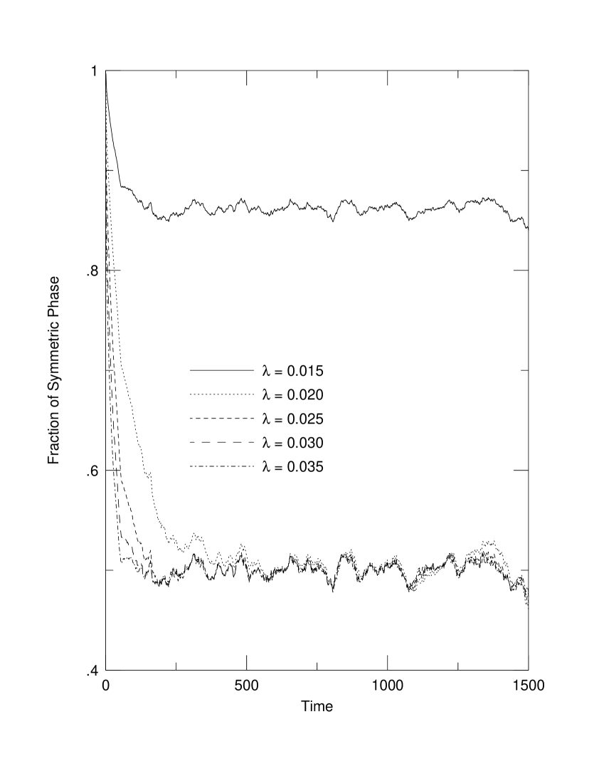
FIG. 5(b): Fraction of the symmetric phase, $f_{0}$, for $\delta x=0.5$.

FIG. 6(a): Correlation function $\left\langle\Phi(\mbox{\boldmath${x}$})\Phi(\mbox{\boldmath${y}$})\right\rangle$ for the scalar field at with the one-loop electroweak potential ($\delta x=1.0$).

FIG. 6(b): Correlation function $\left\langle\Phi(\mbox{\boldmath${x}$})\Phi(\mbox{\boldmath${y}$})\right\rangle$ for the scalar field at with the one-loop electroweak potential ($\delta x=0.5$).

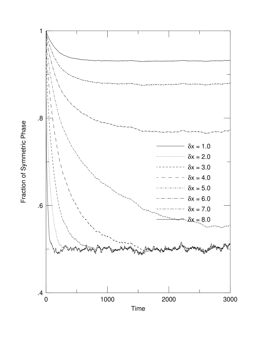
FIG. 7.: Fraction of the symmetric phase, $f_{0}$, for $\delta x$ = 1.0, 2.0, 3.0, 4.0, 5.0, 6.0, 7.0, and 8.0 from the bottom to the top with $\lambda=0.060$.

FIG. 8.: Contribution to $\Gamma$ up to one loop order and ${\cal O}(\lambda^{2},g^{4},f^{2})$. Solid lines represent $\phi$ fields, dotted lines $\chi$ fields, and dashed lines $\psi$ fields.

FIG. 9.: Contribution to $\Gamma$ with two loops order and ${\cal O}(\lambda^{2},g^{4},f^{2})$.

FIG. 10.: Fraction of the symmetric phase, $f_{0}$, for the massless bosonic noise.

FIG. 11.: Fraction of the symmetric, $f_{0}$, phase for the massless fermionic noise.

FIG. 12(a): Snap shot in a plain at $t=1000$ of the simulation with $\delta x=1.0$ and $\lambda=0.02$. Black dots represent asymmetric-state bubbles, while white ones a symmetric-state background.

FIG. 12(b): Snap shot at $t=2000$.

FIG. 12(c): Snap shot at $t=3000$.

FIG. 12(d): Snap shot at $t=4000$.

FIG. 12(e): Snap shot at $t=5000$.

FIG. 13.: Comparison of analytical and numerical results.

FIG. 14.: Fraction of the symmetric, $f_{0}$ starting from a checkerboard.

REFERENCES

- [1]
- [2] G. W. Anderson and L. J. Hall, Phys. Rev. D45, 2685 (1992).
- [3] M. Sher, Phys. Rep. 179, 273 (1989).
- [4] M. Dine, R. G. Leigh, P. Huet, A. Linde, and D. Linde, Phys. Rev. D46, 550 (1992).
- [5] For a review, see, e.g., A. G. Cohen, D. B. Kaplan, and A. E. Nelson, Ann. Rev. and Part. Sci. 43, 27 (1993).
- [6] M. Gleiser, E. W. Kolb, and R. Watkins, Nucl. Phys. B364, 411 (1991).
- [7] M. Gleiser and E. W. Kolb, Phys. Rev. Lett. 69, 1304 (1992)
- [8] M. Gleiser and R. O. Ramos, Phys. Lett. B300, 271 (1993).
- [9] M. Gleiser, Phys. Rev. Lett 73, 3495 (1994).
- [10] J. Borrill and M. Gleiser, Phys. Rev. D51, 4111 (1995).
- [11] T. Shiromizu, M. Morikawa, and J. Yokoyama, Prog. Theor. Phys. 94, 795 (1995); Prog. Theor. Phys. 94, 805 (1995).
- [12] Particle Data Group, Phys. Rev. D54, 1 (1996).
- [13] K. Jansen Nucl. Phys. Proc. Suppl. 47, 196 (1996).
- [14] K. Rummukainen Nucl. Phys. Proc. Suppl. 53, 30 (1997).
- [15] L. M. A. Bettencourt, Phys. Lett. B356, 297 (1995).
- [16] K. Enqvist, A. Riotto, and I. Vilja, Phys. Rev. D52, 5556 (1995).
- [17] J. Schwinger, Jour. Math. Phys. 2, 407 (1961).
- [18] L. V. Keldysh, Zh. Eksp. Teor. Fiz. 47, 1515 (1964).
- [19] M. Morikawa, Phys. Rev. D33, 3607 (1986).
- [20] M. Gleiser and R. O. Ramos, Phys. Rev. D50, 2441 (1994).
- [21] See, e.g., R. J. Rivers, Path Integral Methods in Quantum Field Theory. (Cambridge University Press, Cambridge, 1987) ; D. Boyanovsky and H. J. de Vega, Phys. Rev. D47, 2343 (1993).
- [22] L. Dolan and R. Jackiw, Phys. Rev. D9, 3320 (1974); S. Jeon, Phys. Rev. D47, 4586 (1993); N. P. Landsman and Ch. G. van Weert, Phys. Rep. 145, 141 (1987).
- [23] D. Boyanovsky, H. J. de Vega, R. Holman, D. -S. Lee, and A. Singh, Phys. Rev. D51, 4419 (1995).
- [24] C. Gleiner and B. Müller, hep-th/9605048.
- [25] M. Gleiser, A. F. Heckler, and E. W. Kolb, cond-mat/9512032.
- [26] G. Gelmini and M. Gleiser, Nucl. Phys. B419, 129 (1994).
- [27] M. Alford and M. Gleiser, Phys. Rev. D48, 2838 (1993).
- [28] G. W. Anderson, L. J. Hall, and S. D. H. Hsu, Phys. Lett. B249, 505 (1990).
- [29] G. W. Anderson, Phys. Lett. B295, 32 (1992).