DTP/97/68
UCSD/PTH 97-16
hep-ph/9707496
July 1997

Analytic Calculation of Two Loop Corrections to Heavy Quark
Pair Production Vertices Induced by Light Quarks

A.H. Hoang^a, T. Teubner^b

^a Department of Physics, University of California, San Diego,
La Jolla, CA 92093-0319, USA
^b Department of Physics, University of Durham,
Durham, DH1 3LE, UK

Abstract

Non-singlet ${\cal{O}}(\alpha_{s}^{2})$ corrections from light quarks are calculated analytically for the massive quark-antiquark pair production rates through the vector, axial-vector, scalar and pseudoscalar currents for all energies above the threshold. The results are presented in terms of the moments of the absorptive part of the vacuum polarization function of the light quarks, which allows for an immediate determination of ${\cal{O}}(\alpha_{s}^{2})$ corrections coming from other types of light particles. The kinematic regime close to the threshold is examined, and a comparison to results based on non-relativistic considerations is carried out.
PACS: 12.38.-t, 12.38.Bx, 12.20.Ds
Keywords: Radiative corrections; Fermion pair production; Multi-loop calculation; Four-fermion final state; Method of the moments

1 Introduction

In the past years considerable amount of work has been invested to obtain higher order QCD radiative corrections to quark pair production vertices. As far as the quark pair production rates through the vector and axial-vector currents are concerned this effort was mainly motivated by the impressive amount of data on hadronic Z decay events obtained at the LEP experiments. Whereas the ${\cal{O}}(\alpha_{s})$ corrections have been well known since quite a long time for all energy and mass values [1, 2], the complete analytic form of the ${\cal{O}}(\alpha_{s}^{2})$ corrections is known as a high energy expansion in $M^{2}/q^{2}$ [3], where $\sqrt{q^{2}}$ denotes the c.m. energy and $M$ the mass of the produced quarks. For high energies, even the leading leading ${\cal{O}}(\alpha_{s}^{3})$ [4] and some mass corrections have been calculated [5]. The quark pair production rates through the scalar and pseudoscalar currents have also been investigated in view of the expected studies of hadronic Higgs decays at forthcoming collider experiments. Here, the ${\cal{O}}(\alpha_{s})$ corrections are well established for all ratios $M^{2}/q^{2}$ [6, 7], while the second order corrections are known as an expansion in $M^{2}/q^{2}$ [8]. Thus, to ${\cal{O}}(\alpha_{s}^{2})$ the present calculations are definitely a good approximation if the c.m. energy is much larger than the mass of the produced fermions, which is for example the case for $Z$ or Higgs decays into bottom quarks, but can also be applied for intermediate energies if a sufficient number of terms in the high energy expansion is taken into account (see also [9] for a review). However, in face of forthcoming experiments ($\tau$-charm-, B-factory, NLC), where quark pairs will also be produced in the kinematic regime where the quark masses and the c.m. energy are of comparable order, i.e. closer to the threshold, the knowledge of the entire ${\cal{O}}(\alpha_{s}^{2})$ corrections valid for all values of $M^{2}/q^{2}$ is desirable. Whereas meanwhile there are methods to obtain numerical approximations for the ${\cal{O}}(\alpha_{s}^{2})$ corrections in the latter kinematic regime based on Padé approximants [10], the entire analytic calculation seems to be an impossible task at the present stage. However, analytical results are of particular importance because they provide important cross checks for approximation methods and serve as a starting point for qualitative considerations.

A first step towards a complete analytical calculation consists of the determination of those ${\cal{O}}(\alpha_{s}^{2})$ corrections to the heavy quark production vertices which are induced by light quarks. These corrections are equal to the sum of all possible cuts of at least two massive quark lines of current-current correlator diagrams consisting of a massive quark loop, a massless quark loop and two gluon lines. The individual contributions can be divided into three classes: (i) the massive quarks are produced directly by the external current insertion (primary production), (ii) the massive quarks are produced via gluon emission off the massless quarks (secondary production) and (iii) the interference between amplitudes of class (i) and (ii). Class (iii) corresponds to cuts of the double-triangle or singlet diagrams. For the vector current correlator the class (iii) diagrams vanish due to Furry’s theorem. The contributions belonging to class (ii) were determined analytically in [11, 12] for the vector and axial-vector case.

In this work we present analytic expressions for the ${\cal{O}}(\alpha_{s}^{2})$ corrections belonging to class (i) for arbitrary values of the quark mass $M$ and c.m. energy $\sqrt{q^{2}}$ above threshold. Analytic formulae for primary production through the vector and scalar currents were already presented in [14] and [15], respectively. Here we carry out the same program for the axial-vector and pseudoscalar case. In addition, we present the results in terms of moments of the absorptive part of the vacuum polarization of the light quark-antiquark pair, proceeding along the lines of [16], which allows for an immediate determination of the ${\cal{O}}(\alpha_{s}^{2})$ corrections coming from light colored scalar particles or from the gluonic vacuum polarization insertion. Based on the concept of the moments even a certain class of ${\cal{O}}(\alpha_{s}^{3})$ and ${\cal{O}}(\alpha_{s}^{4})$ corrections can be determined. Thus, for completeness also the vector and scalar cases are presented in terms of the moments.

To be definite we consider the light quark induced ${\cal{O}}(\alpha_{s}^{2})$ contributions to the imaginary part of the massive quark current-current correlators

$$\Pi^{\Theta}_{\mu\nu}(q) = -\,i\int\!{\rm d}x\,e^{i\,q.x}\,\langle 0|\,T\,j^{\Theta}_{\mu}(x)\,j^{\Theta}_{\nu}(0)\,|0\rangle$$ (1)

$$= g_{\mu\nu}\,q^{2}\,\Pi^{\Theta}(q^{2})-q_{\mu}\,q_{\nu}\,\Pi_{L}^{\Theta}(q^{2})\,,\qquad\Theta=V,A,$$

for the vector and the axial-vector currents

$$j_{\mu}^{V}\,=\,\bar{\Psi}_{Q}^{0}\,\gamma_{\mu}\,\Psi_{Q}^{0}\,,\qquad\qquad j_{\mu}^{A}\,=\,\bar{\Psi}_{Q}^{0}\,\gamma_{\mu}\,\gamma_{5}\,\Psi_{Q}^{0}\,,$$ (2)

and

$$q^{2}\,\Pi^{\Theta}(q^{2}) = i\int\!{\rm d}x\,e^{i\,qx}\,\langle 0|\,T\,j^{\Theta}(x)\,j^{\Theta}(0)\,|0\rangle\,,\qquad\Theta=S,P,$$ (3)

for the scalar and pseudoscalar currents

$$j^{S}\,=\,M^{0}\,\bar{\Psi}_{Q}^{0}\,\Psi_{Q}^{0}\,,\qquad\qquad j^{P}\,=\,i\,M^{0}\,\bar{\Psi}_{Q}^{0}\,\gamma_{5}\,\Psi_{Q}^{0}\,,$$ (4)

where summation over color degrees of freedom is understood. $\Psi_{Q}^{0}$ denotes the bare massive quark field and $M^{0}$ its bare mass. In order to maintain vanishing anomalous dimension for all four currents the scalar and pseudoscalar currents are defined including the mass parameter. The longitudinal part of the vector current correlator $\Pi_{L}^{V}$ is equal to $\Pi^{V}$ due to current conservation, whereas $\Pi_{L}^{A}$ is related to the pseudoscalar current correlator $\Pi^{P}$ via the axial Ward identity. The optical theorem relates the renormalization group invariant imaginary parts of $\Pi^{\Theta}$, $\Theta=V,A,S,P$, to decay rates and cross-sections. The contribution of ${\rm Im}\Pi^{V,A}$ to the total hadronic Z decay rate reads

$$\Delta\,\Gamma_{Z}^{had} = \frac{G_{F}\,M_{Z}^{3}}{24\,\sqrt{2}\,\pi}\,\left(\,v_{Q}^{2}\,R^{V}(M_{Z}^{2})+a_{Q}^{2}\,R^{A}(M_{Z}^{2})\,\right)\,,$$ (5)

$$a_{Q} = 2\,I_{3}^{Q}\,,$$

$$v_{Q} = 2\,I_{3}^{Q}-4\,q_{Q}\,\sin^{2}\theta_{W}\,,$$

where

$$R^{A,V}(q^{2})\,\equiv\,12\,\pi\,{\rm Im}\Pi^{A,V}(q^{2}+i\,\epsilon)\,,$$ (6)

$q_{Q}$ is the massive quark electric charge, $\Theta_{W}$ the Weinberg angle and $I_{3}^{Q}$ the massive quark weak isospin. Moreover, $R^{V}$ is equal to the cross-section of $Q\bar{Q}$ production in $e^{+}e^{-}$ annihilation into a single photon normalized to the point cross-section. The contribution of the quantities $R^{V,A}$ to Z-mediated $Q\bar{Q}$ production is straightforward. The contributions of ${\rm Im}\Pi^{S,P}$ to the hadronic decay widths of a scalar or pseudoscalar Higgs boson with mass $m_{S}$ and $m_{P}$, respectively, read

$$\Delta\,\Gamma_{S,P}^{had}\,=\,\frac{G_{F}\,M^{2}}{4\,\sqrt{2}\,\pi}\,m_{S,P}\,a_{S,P}^{F}\,R^{S,P}(m_{S,P}^{2})\,,$$ (7)

where

$$R^{S,P}(q^{2})\,\equiv\,\frac{8\,\pi}{M^{2}}\,{\rm Im}\Pi^{S,P}(q^{2}+i\,\epsilon)$$ (8)

and $M$ denotes the heavy quark pole mass. The coefficient $a_{S,P}^{F}$ is the relative weight of the corresponding partial width with respect to the standard model Higgs decay rate ($a_{H}^{F}=1$). Thus in the framework of the MSSM, where a two doublet Higgs sector is realized, $a_{H}^{up}=\sin^{2}\alpha/\sin^{2}\beta$, $a_{H}^{down}=\cos^{2}\alpha/\cos^{2}\beta$, $a_{h}^{up}=\cos^{2}\alpha/\sin^{2}\beta$, $a_{h}^{down}=\sin^{2}\alpha/\cos^{2}\beta$, $a_{A}^{up}=\cot^{2}\beta$ and $a_{A}^{down}=\tan^{2}\beta$, where $H,h$ and $A$ denote the heavy and light scalar and the pseudoscalar Higgs fields, respectively. $\alpha$ describes the mixing between the two Higgs doublets and $\beta$ is defined via the ratio of their vacuum expectation values, $\tan\beta=v_{2}/v_{1}$ (see e.g. [17]). In the following sections we present the results of our calculation in terms of the quantities $R^{\Theta}$, $\Theta=V,A,S,P$. Their perturbative expansion using the $\overline{\rm MS}$ renormalization scheme for the strong coupling reads

$$R^{\Theta}(q^{2})\,=\,r_{\Theta}^{(0)}(q^{2})+\left(\frac{\alpha_{s}^{\overline{\mbox{\tiny MS}}}(\mu^{2})}{\pi}\right)\,r_{\Theta}^{(1)}(q^{2})+\left(\frac{\alpha_{s}^{\overline{\mbox{\tiny MS}}}(\mu^{2})}{\pi}\right)^{2}\,r_{\Theta}^{(2),{\overline{\mbox{\tiny MS}}}}(q^{2},\mu^{2})+\ldots\,,$$ (9)

where the light quark ${\cal{O}}(\alpha_{s}^{2})$ corrections determined in this work will be referred to as $r_{\Theta,q}^{(2),{\overline{\mbox{\tiny MS}}}}$. As we use the pole definition for the heavy mass $M$ throughout this work, only the ${\cal{O}}(\alpha_{s}^{2})$ coefficient of $R_{\Theta}$ is renormalization group $\mu$-dependent. For simplicity we call the quantities $R^{\Theta}$, $\Theta=V,A,S,P$, decay rates from now on in this paper. Because the calculations for the virtual light quark corrections are most easily performed by using dispersion integration techniques, the results for all four heavy quark currents are derived in the framework of on-shell renormalized QED, where the coupling $\alpha$ is defined as the fine structure constant and the wave function renormalization constant of the quark fields is fixed by the requirement that the residue of the fermion propagator is one. In a second separate step the results are then transferred to the QED $\overline{\rm MS}$ scheme for the coupling and to QCD. Throughout this paper the heavy quark will be denoted as $Q$ with pole mass $M$ and the light quarks as $q$ with mass $m$. It should also be noted that, even in the framework of QED, we will refer to the fermions as quarks though they may be leptons as well. For simplicity all quarks are assigned electric charge one. The generalization to different charge assignments is straightforward. All QED results are marked with a tilde.

The program of this work is as follows: in Section 2 we describe in some detail the calculation of the light quark ${\cal O}(\alpha^{2})$ corrections to massive quark pair production through the vector current in on-shell QED. Virtual and real contributions as well as the inclusive sum are discussed separately. The results are presented in a general form which is common for all the cases ($V,A,S,P$). The corresponding results for corrections to axial vector induced quark pair production are then given in Section 3, whereas in Section 4 the cases of scalar and pseudoscalar currents are treated on the same footing. In Section 5 we carry out the transition from on-shell QED to the $\overline{\rm MS}$ scheme and to QCD. As mentioned above our results are presented in terms of moments of the inserted vacuum polarization from light quarks. In Section 6 this “method of the moments” is discussed in more detail. We present the corresponding moments for light scalar and gluonic second order corrections. Section 7 contains a discussion of our results in the threshold region and Section 8 our summary. For the sake of completeness numerous ${\cal{O}}(\alpha)$ formulae for the cases of the different currents ($V,A,S,P$) are given in Appendix A. Second order virtual corrections in the case of equal masses $m=M$ are listed in Appendix B. For the convenience of the reader we also present expansions for the high energy as well as for the threshold region in Appendix C. Phenomenological applications of the results will be discussed elsewhere.

2 Heavy Quark Production through the Vector Current

2.1 Virtual Corrections

The virtual light quark ${\cal{O}}(\alpha^{2})$ corrections to the massive quark production vertex induced by the vector current correspond to the sum of the two particle cuts of the current-current correlator diagrams depicted in Fig. 1. This leads to virtual photon exchange diagrams with an additional vacuum polarization insertion of a light quark-antiquark pair.

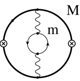
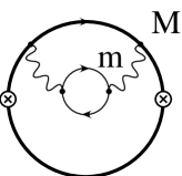
Figure 1: Double bubble diagrams where a pair of heavy quarks of mass $M$ is produced through an external current. The exchanged photon splits into the light quark-antiquark pair of mass $m$.

The basic idea is to write the light quark-antiquark contributions to the photon vacuum polarization function $\tilde{\Pi}^{\mu\nu}$ in terms of an one-time subtracted dispersion relation (which accounts for the correct subtraction of the subdivergence in the light quark vacuum polarization),

$$\tilde{\Pi}^{\mu\nu}_{q\bar{q}}(m^{2},q^{2}) = -i\,\Big{(}g^{\mu\nu}\,q^{2}-q^{\mu}\,q^{\nu}\Big{)}\,\tilde{\Pi}^{q}(m^{2},q^{2})\,,$$ (10)

$$\tilde{\Pi}^{q}(m^{2},q^{2}) = \frac{1}{3}\,\bigg{(}\frac{\alpha}{\pi}\bigg{)}\,q^{2}\int\limits_{4\,m^{2}}^{\infty}\,\frac{{\rm d}{\lambda}^{2}}{{\lambda}^{2}\,({\lambda}^{2}-q^{2}-i\epsilon)}\,\tilde{R}_{q\bar{q}}(m^{2},\lambda^{2})\,,$$ (11)

where

$$\tilde{R}_{q\bar{q}}(m^{2},q^{2})\,=\,\sqrt{1-4\,\frac{m^{2}}{q^{2}}}\,\left(\,1+2\,\frac{m^{2}}{q^{2}}\,\right)$$ (12)

is the absorptive part of the vacuum polarization function of the light quark-antiquark pair. Thus the effective propagator which has to be inserted into the virtual photon line can be written as

$$\frac{-i}{q^{2}+i\epsilon}\left(g^{\mu\sigma}-\xi\frac{q^{\mu}\,q^{\sigma}}{q^{2}}\right)\,\tilde{\Pi}^{q\bar{q}}_{\sigma\rho}(m^{2},q^{2})\,\frac{-i}{q^{2}+i\epsilon}\left(g^{\rho\nu}-\xi\frac{q^{\rho}\,q^{\nu}}{q^{2}}\right)$$ (13)

$$= \frac{1}{3}\left(\frac{\alpha}{\pi}\right)\int\limits_{4\,m^{2}}^{\infty}\frac{{\rm d}\lambda^{2}}{\lambda^{2}}\,\bigg{[}\frac{-\,i\,g^{\mu\nu}}{q^{2}-\lambda^{2}+i\epsilon}\bigg{]}\,\tilde{R}_{q\bar{q}}(m^{2},\lambda^{2})\,+\ldots\,\,.$$

The longitudinal terms indicated by the dots are irrelevant due to current conservation. It is evident from Eq. (13) that the effective propagator is a convolution of a massive vector boson propagator in Feynman gauge with the function $\tilde{R}_{q\bar{q}}$. Inserting expression (13) into the vertex diagrams and carrying out the vertex loop integration first, the intended two-loop corrections can be written as a convolution integration over the corresponding ${\cal{O}}(\alpha)$ virtual corrections with exchange of a massive vector boson of mass $\lambda$.

It is customary to parameterize the virtual corrections to the renormalized vector current vertex $\Lambda_{\mu}^{V}$ in terms of the Dirac ($F_{1}$) and the Pauli ($F_{2}$) form factors

$$\overline{u}_{Q}(k_{2})\,\Lambda_{\mu}^{V}\,v_{Q}(k_{1})\,=\,\overline{u}_{Q}(k_{2})\,\left[\,\gamma_{\mu}\,F_{1}(q^{2})+\frac{i}{2\,M}\,\sigma_{\mu\nu}\,q^{\nu}\,F_{2}(q^{2})\,\right]\,v_{Q}(k_{1})\,,$$ (14)

where $q=k_{1}+k_{2}$, $\sigma_{\mu\nu}=\frac{i}{2}[\gamma_{\mu},\gamma_{\nu}]$. $u_{Q}$ and $v_{Q}$ denote the free heavy quark and antiquark Dirac fields, respectively. The perturbative expansions of the form factors read

$$F_{1}(q^{2}) = 1+\left(\frac{\alpha}{\pi}\right)\,F_{1}^{(1)}(q^{2})+\left(\frac{\alpha}{\pi}\right)^{2}\,F_{1}^{(2)}(q^{2})+\ldots\,,$$ (15)

$$F_{2}(q^{2}) = \hskip 18.49411pt\left(\frac{\alpha}{\pi}\right)\,F_{2}^{(1)}(q^{2})+\left(\frac{\alpha}{\pi}\right)^{2}\,F_{2}^{(2)}(q^{2})+\ldots\,.$$ (16)

The Dirac form factor is normalized to one at zero momentum transfer $q^{2}=0$ at all orders in $\alpha$. To ${\cal{O}}(\alpha)$ this is completely achieved by the on-shell QED quark field wave function renormalization constant, which is fixed by the requirement that the residue of the renormalized heavy quark propagator is one. No further subtraction is required because the vector current as defined in Eq. (2) is anomalous dimension free. Based on the considerations presented above, the light quark corrections to the ${\cal{O}}(\alpha^{2})$ form factors can be written as an one-dimensional integral,

$$F_{i,q}^{(2)}(M^{2},m^{2},q^{2})=\frac{1}{3}\int\limits_{4\,m^{2}}^{\infty}\frac{{\rm d}\lambda^{2}}{\lambda^{2}}\,F_{i}^{(1)}(M^{2},q^{2},\lambda^{2})\,\tilde{R}_{q\bar{q}}(m^{2},\lambda^{2})\,,\qquad i=1,2\,,$$ (17)

where $F_{1/2}^{(1)}(M^{2},q^{2},\lambda)$ denotes the first order form factors with virtual exchange of a vector boson with mass $\lambda$. In Eq. (17) we have indicated the mass dependence of the form factors explicitly in order to illustrate the mass dependence of the individual factors. It should be noted that the light quark corrections to the ${\cal{O}}(\alpha^{2})$ form factors, Eq. (17), are already renormalized properly and that no additional subtraction is needed. In particular, the subdivergence from the virtual light quark loop is taken care of properly by using the subtracted dispersion relation in the $\lambda^{2}$ integration, whereas the overall divergences are subtracted correctly in the ${\cal{O}}(\alpha)$ form factors. The same remark holds also true for the corresponding virtual light quark ${\cal{O}}(\alpha^{2})$ corrections for the axial-vector, scalar and pseudoscalar cases presented in the subsequent sections.

The contributions of the form factors to the decay rate

$$\tilde{R}^{V}(q^{2})\,=\,\tilde{r}_{V}^{(0)}(q^{2})+\left(\frac{\alpha}{\pi}\right)\,\tilde{r}_{V}^{(1)}(q^{2})+\left(\frac{\alpha}{\pi}\right)^{2}\,\tilde{r}_{V}^{(2)}(q^{2})+\ldots$$ (18)

read

$$\tilde{r}_{V}^{(0)}(q^{2}) = \frac{1}{2}\,\beta\,(3-\beta^{2})\,,$$ (19)

$$\tilde{r}_{V}^{(1),virt}(q^{2}) = \beta\,(3-\beta^{2})\,\left(\,{\rm Re}F_{1}^{(1)}(q^{2})+{\rm Re}F_{2}^{(1)}(q^{2})\,\right)+\beta^{3}\,{\rm Re}F_{2}^{(1)}(q^{2})\,,$$ (20)

where

$$\beta\,=\,\sqrt{1-4\,\frac{M^{2}}{q^{2}}}$$

is the velocity of the massive quarks in the c.m. frame.

The contribution of $F_{1/2,q}^{(2)}$ to $\tilde{r}_{V}^{(2)}$ is given by

$$\tilde{r}_{V,q}^{(2),virt}(q^{2})\,=\,\beta\,(3-\beta^{2})\,\left(\,{\rm Re}F_{1,q}^{(2)}(q^{2})+{\rm Re}F_{2,q}^{(2)}(q^{2})\,\right)+\beta^{3}\,{\rm Re}F_{2,q}^{(2)}(q^{2})\,.$$ (21)

The real parts of $F_{1/2}^{(1)}(M^{2},q^{2},\lambda^{2})$ have already been presented in [14, 18]. For the convenience of the reader the full form of the ${\cal{O}}(\alpha)$ form factors with massive vector boson exchange above threshold is presented in Appendix A.1, Eqs. (153) and (154). For $\lambda^{2}\to 0$ the expressions for the ${\cal{O}}(\alpha)$ form factors relevant for $r_{V}^{(1),virt}$ are obtained. This results in the well known QED expressions calculated by [1], where the IR singularity in $F_{1}$ is regularized by the small fictitious photon mass $\lambda$,

$$F_{1}^{(1)}(M^{2},q^{2},\lambda^{2}\rightarrow 0)\,=\,$$ (22)

$$\mbox{}-\frac{1}{2}\,\bigg{(}1+\frac{1+{{\beta}^{2}}}{2\,\beta}\,\ln p\bigg{)}\,\ln\frac{\lambda^{2}}{M^{2}}-\frac{1+{{\beta}^{2}}}{2\,\beta}\,\left(\mbox{Li}_{2}(1-p)+\frac{1}{4}\,\ln^{2}p-3\,\zeta(2)\right)\,\,$$

$$\mbox{}-\frac{1+2\,{{\beta}^{2}}}{4\,\beta}\,\ln p-1-i\,\pi\,\bigg{[}\,\frac{1+{{\beta}^{2}}}{4\,\beta}\,\ln\frac{\lambda^{2}}{M^{2}}+\frac{1+{{\beta}^{2}}}{4\,\beta}\,\ln\Big{(}\frac{1-{{\beta}^{2}}}{4\,{{\beta}^{2}}}\Big{)}+\frac{1+2\,{{\beta}^{2}}}{4\,\beta}\,\bigg{]}\,,$$

$$F_{2}^{(1)}(M^{2},q^{2},\lambda^{2}\rightarrow 0)\,=\,\frac{1-{\beta^{2}}}{4\,\beta}\,\Big{(}\ln p+i\,\pi\Big{)}\,,$$ (23)

where

$$p\,=\,\frac{1-\beta}{1+\beta}\,.$$

For arbitrary ratios $m/M$ the evaluation of Eq. (17) can be carried out, but is extremely tedious. However, in the case of interest, $m/M\to 0$, the task can be simplified enormously by subtracting and adding $\tilde{R}_{q\bar{q}}$ at its asymptotic value at high energies, $\tilde{R}_{\infty}^{q}\equiv\tilde{R}_{q\bar{q}}(m^{2},q^{2}=\infty)$:

$$F_{i,f}^{(2)}(M^{2},m^{2},q^{2}) = \frac{1}{3}\int\limits_{4\,m^{2}}^{\infty}\frac{{\rm d}\lambda^{2}}{\lambda^{2}}\,F_{i}^{(1)}(M^{2},q^{2},\lambda^{2})\,\left[\tilde{R}_{q\bar{q}}(m^{2},\lambda^{2})-\tilde{R}_{\infty}^{q}\right]$$ (24)

$$\,+\,\frac{1}{3}\,\tilde{R}_{\infty}^{q}\int\limits_{4\,m^{2}}^{\infty}\frac{{\rm d}\lambda^{2}}{\lambda^{2}}\,F_{i}^{(1)}(M^{2},q^{2},\lambda^{2})\,,\qquad i=1,2\,.$$

Because $\tilde{R}_{q\bar{q}}$ reaches its asymptotic value already for values of $\lambda^{2}$ much smaller than the heavy scales $M^{2}$ and $q^{2}$, which govern the ${\cal{O}}(\alpha)$ form factors, we can replace $F_{1/2}^{(1)}(M^{2},q^{2},\lambda^{2})$ in the first integral on the r.h.s. of (24) by the QED expressions for $\lambda^{2}\to 0$, Eqs. (22) and (23). The resulting integration can then be trivially expressed in terms of the moments $\tilde{R}_{0}^{q}$ and $\tilde{R}_{1}^{q}$ defined by

$$\tilde{R}_{n}^{q}\,=\,\frac{1}{n!}\int\limits_{0}^{1}{\rm d}x\,\frac{\ln^{n}x}{x}\,\Big{[}\,\tilde{R}_{q\bar{q}}\Big{(}m^{2},\frac{4\,m^{2}}{x}\Big{)}-\tilde{R}_{\infty}^{q}\,\Big{]}\,,\qquad n=0,1,2,\ldots\,.$$ (25)

The evaluation of the second integral on the r.h.s. of (24) constitutes the main effort. The final results for the light quark ${\cal{O}}(\alpha^{2})$ corrections to the form factors can be cast into the form ($x=q$)

$$F_{1,x}^{(2)} = f_{1}^{(2)}\,\bigg{[}\,\tilde{R}_{\infty}^{x}\,\ln^{2}\frac{m^{2}}{q^{2}}-2\,\tilde{R}_{0}^{x}\,\ln\frac{m^{2}}{q^{2}}+2\,\tilde{R}_{1}^{x}\,\bigg{]}+f_{1}^{(1)}\,\bigg{[}\,\tilde{R}_{\infty}^{x}\,\ln\frac{m^{2}}{q^{2}}-\tilde{R}_{0}^{x}\,\bigg{]}+f_{1}^{(0)}\,\tilde{R}_{\infty}^{x}\,,$$ (26)

$$F_{2,x}^{(2)} = f_{2}^{(1)}\,\bigg{[}\,\tilde{R}_{\infty}^{x}\,\ln\frac{m^{2}}{q^{2}}-\tilde{R}_{0}^{x}\,\bigg{]}+f_{2}^{(0)}\,\tilde{R}_{\infty}^{x}\,,$$ (27)

where

$$f_{1}^{(0)} = A_{virt}+\frac{2}{3}\,(1+2\,{{\beta}^{2}})\,B_{virt}-\frac{1}{3}\,\ln\Big{(}\frac{1-{{\beta}^{2}}}{16}\Big{)}+\frac{5+2\,{{\beta}^{2}}}{24\,\beta}\,\ln p-\frac{1-\beta+2\,{{\beta}^{2}}}{2\,\beta}\,\zeta(2)+\frac{1}{6}$$

$$+i\,\pi\,\biggl{\{}\,\frac{1}{12\,\beta}\,\biggl{[}\,2\,(1+{{\beta}^{2}})\,\ln^{2}\Big{(}\frac{\beta}{2}\Big{)}-2\,(1+2\,{{\beta}^{2}})\,\ln\Big{(}\frac{\beta}{2}\Big{)}+(1+{{\beta}^{2}})\,\zeta(2)+\frac{1}{2}\,(5+2\,{{\beta}^{2}})\,\biggr{]}\,\biggr{\}}\,,$$

$$f_{1}^{(1)} = \frac{2}{3}\,(1+{{\beta}^{2}})\,B_{virt}-\frac{1}{6}\,\ln\Big{(}\frac{1-{{\beta}^{2}}}{16}\Big{)}+\frac{1+2\,{{\beta}^{2}}}{12\,\beta}\,\ln p-\frac{1+{{\beta}^{2}}}{2\,\beta}\,\zeta(2)+\frac{1}{3}$$ (29)

$$+i\,\pi\,\biggl{\{}\,\frac{1}{12\,\beta}\,\biggl{[}\,-2\,(1+{{\beta}^{2}})\,\ln\Big{(}\frac{\beta}{2}\Big{)}+1+2\,{{\beta}^{2}}\,\biggr{]}\,\biggr{\}}\,,$$

$$f_{1}^{(2)} = \frac{1+{{\beta}^{2}}}{24\,\beta}\,\ln p+\frac{1}{12}\,+\,i\,\pi\,\biggl{\{}\,\frac{1+{{\beta}^{2}}}{24\,\beta}\,\biggr{\}}\,,$$ (30)

$$f_{2}^{(0)} = -\frac{2}{3}\,(1-{{\beta}^{2}})\,B_{virt}-\frac{5\,\left(1-{{\beta}^{2}}\right)}{24\,\beta}\,\ln p+\frac{1-{{\beta}^{2}}}{2\,\beta}\,\zeta(2)\,+\,i\,\pi\,\biggl{\{}\,\frac{1-{{\beta}^{2}}}{6\,\beta}\,\biggl{[}\,\ln\Big{(}\frac{\beta}{2}\Big{)}-\frac{5}{4}\,\biggr{]}\,\biggr{\}}\,,$$ (31)

$$f_{2}^{(1)} = -\frac{1-{{\beta}^{2}}}{12\,\beta}\,\ln p\,+\,i\,\pi\,\biggl{\{}\,-\frac{1-{{\beta}^{2}}}{12\,\beta}\,\biggr{\}}\,,$$ (32)

and

$$A_{virt} = -\frac{1+{{\beta}^{2}}}{6\,\beta}\,\bigg{[}\,2\,\mbox{Li}_{3}(1-p)+\mbox{Li}_{3}(p)+\mbox{Li}_{2}(1-p)\,\ln\Big{(}\frac{1-{{\beta}^{2}}}{16}\Big{)}\,$$ (33)

$$\mbox{}\,\qquad\quad\qquad-\frac{1}{12}\,\ln^{3}p+\frac{1}{2}\,\ln^{2}p\,\ln\Big{(}2\,(1-{p^{2}})\Big{)}-\ln p\,\ln^{2}\Big{(}2\,(1+p)\Big{)}\,\,$$

$$\mbox{}\,\qquad\quad\qquad-2\,\bigg{(}3\,\ln\Big{(}\frac{\beta}{2}\Big{)}+\frac{5}{4}\,\ln p\bigg{)}\,\zeta(2)-\zeta(3)\,\bigg{]}+\frac{1}{12}\,\ln^{2}\Big{(}\frac{1-{{\beta}^{2}}}{16}\Big{)}\,,$$

$$B_{virt} = \frac{1}{4\,\beta}\,\bigg{[}\,\mbox{Li}_{2}(1-p)+\ln p\,\bigg{(}\ln(1+p)-\frac{1}{4}\,\ln p+\ln 2\bigg{)}\,\bigg{]}\,.$$ (34)

In [14] the real parts of the form factors were already presented in a somewhat more implicit form. The light quark-antiquark moments read

$$\tilde{R}_{\infty}^{q} = 1\,,$$

$$\tilde{R}_{0}^{q} = \ln 4-\frac{5}{3}\,,$$

$$\tilde{R}_{1}^{q} = \frac{1}{2}\ln^{2}4-\frac{5}{3}\ln 4+\frac{28}{9}-\zeta(2)\,,$$

$$\tilde{R}_{2}^{q} = \frac{1}{6}\,\ln^{3}4-\frac{5}{6}\,\ln^{2}4+\bigg{(}\,\frac{28}{9}-\zeta(2)\,\bigg{)}\,\ln 4-\frac{164}{27}+\frac{5}{3}\,\zeta(2)+2\,\zeta(3)\,.$$ (35)

The reader should note that the entire information on the light quark-antiquark vacuum polarization inserted into the photon line is encoded in the three moments $\tilde{R}_{\infty}^{q}$, $\tilde{R}_{0}^{q}$ and $\tilde{R}_{1}^{q}$. For completeness we have also given the moment $\tilde{R}_{2}^{q}$. At this point we would like to mention that the definition of the moments of the light quark-antiquark vacuum polarization, as given in Eq. (25), strongly relies on the dispersion integration approach we used to determine the light quark ${\cal{O}}(\alpha^{2})$ corrections to the form factors. In this approach the occurrence of higher moments $\tilde{R}_{n}^{q}$, $n\geq 1$, comes from infrared singular terms $\propto\ln^{n}\lambda$ in the ${\cal{O}}(\alpha)$ form factors for $\lambda\to 0$. If, on the other hand, dimensional regularization is employed to regularize ultraviolet as well as infrared divergences, the moments (35) can be uniquely identified from the renormalized high energy vacuum polarization function in arbitrary $D=4-2\epsilon$ dimension. Expanded in terms of small $\epsilon$ the vacuum polarization function in the limit $q^{2}/m^{2}\to\infty$ ($m$ being the light quark pole mass and $\alpha$ the fine structure constant) reads ($x=q$)

$$\tilde{\Pi}_{light}^{x}(q^{2})\,=\,-\frac{\alpha}{3\,\pi}\,\bigg{\{}\,\bigg{[}\,\tilde{R}_{0}^{x}+\tilde{R}_{\infty}^{x}\,\ln\frac{-q^{2}}{4\,m^{2}}\,\bigg{]}$$ (36)

$$\qquad-\,\epsilon\,\bigg{[}\,\tilde{R}_{1}^{x}+\Big{(}\tilde{R}_{\infty}^{x}\,\ln\frac{-q^{2}}{4\,m^{2}}+\tilde{R}_{0}^{x}\Big{)}\,\ln\frac{-q^{2}}{4\,\mu^{2}}-\frac{1}{2}\,\tilde{R}_{\infty}^{x}\,\ln^{2}\frac{-q^{2}}{4\,m^{2}}\,\bigg{]}\,$$

$$\qquad+\,\epsilon^{2}\,\bigg{[}\,\tilde{R}_{2}^{x}+\frac{1}{2}\,\Big{(}\tilde{R}_{\infty}^{x}\,\ln\frac{-q^{2}}{4\,m^{2}}+\tilde{R}_{0}^{x}\Big{)}\,\Big{(}\ln^{2}\frac{-q^{2}}{4\,\mu^{2}}+\zeta(2)\Big{)}$$

$$\qquad\qquad-\Big{(}\frac{1}{2}\,\tilde{R}_{\infty}^{x}\,\ln^{2}\frac{-q^{2}}{4\,m^{2}}-\tilde{R}_{1}^{x}\Big{)}\,\ln\frac{-q^{2}}{4\,\mu^{2}}+\frac{1}{6}\,\tilde{R}_{\infty}^{x}\,\ln^{3}\frac{-q^{2}}{4\,m^{2}}\,\bigg{]}\,\bigg{\}}+\,{\cal{O}}(\epsilon^{3})\,,$$

where $\mu$ is the common scale parameter introduced in dimensional regularization. Thus, in the framework of dimensional regularization higher moments $\tilde{R}_{n}^{q}$, $n\geq 1$, in the expression for the second order form factors come from $(1/\epsilon)^{n}$ infrared divergences in the ${\cal{O}}(\alpha)$ form factors which cancel the corresponding $\epsilon^{n}$ terms in $\tilde{\Pi}_{light}^{q}$.

2.2 Real Radiation

The ${\cal{O}}(\alpha^{2})$ corrections from real radiation of a light quark-antiquark pair in primary massive quark pair production correspond to the sum of all four body cuts of the diagrams shown in Fig. 1 and represent the Born rate for primary massive quark production with additional radiation of a light quark-antiquark pair. In order to accommodate for the conventions used in the calculation of the virtual corrections we will for now remain in the framework of on-shell QED for the calculation of the real radiation process. Again we will determine the contribution to the imaginary part of the current-current correlator (1), denoted by $\tilde{r}_{V,q}^{(2),real}$. This task is accomplished by dividing the four-body phase space into three different subprocesses: radiation of a photon with virtuality $\lambda^{2}$ off one of the massive quarks, propagation of the photon and decay of the virtual photon into the light quark-antiquark pair. The first process is described by $\tilde{r}_{V}^{(1),real}(M^{2},q^{2},\lambda^{2})$, the ${\cal{O}}(\alpha)$ contribution to the decay rate $R^{V}$, Eq. (9), from real radiation of a photon with virtuality (mass squared) $\lambda^{2}$. The third process is proportional to $\tilde{R}_{q\bar{q}}$, Eq. (12). Combining both contributions with the photon propagation function, summing over all photon polarizations and integrating over all allowed values of $\lambda^{2}$, we arrive at the expression

$$\tilde{r}_{V,q}^{(2),real}(M^{2},m^{2},q^{2})\,=\,\frac{1}{3}\int\limits_{4\,m^{2}}^{(\sqrt{q^{2}}-2\,M)^{2}}\frac{{\rm d}\lambda^{2}}{\lambda^{2}}\,\,\tilde{r}_{V}^{(1),real}(M^{2},q^{2},\lambda^{2})\,\,\tilde{R}_{q\bar{q}}(m^{2},\lambda^{2})\,.$$ (37)

It is evident that Eq. (37) closely resembles the corresponding formula for the virtual light quark ${\cal{O}}(\alpha^{2})$ corrections, Eq. (17). An integral representation of $\tilde{r}_{V}^{(1),real}(M^{2},q^{2},\lambda^{2})$ can be found in Appendix A.1. For $\lambda^{2}\to 0$ the well known QED result of [1] is recovered:

$$\tilde{r}_{V}^{(1),real}(M^{2},q^{2},\lambda^{2}) \stackrel{{\scriptstyle\lambda^{2}\to 0}}{{\longrightarrow}} 6\,f_{V}^{(2),real}\,\Big{[}\,\ln\frac{4\,q^{2}}{{{\lambda}^{2}}}\,\Big{]}-3\,f_{V}^{(1),real}\,,$$ (38)

where the functions $f_{V}^{(2),real}$ and $f_{V}^{(1),real}$ are given below (see Eqs. (43) and (44)). It should be noted that the leading infrared behavior for $m/M\to 0$ of expression (37) is determined by the logarithmic photon mass singularity in Eq. (38). For arbitrary masses $m$ and $M$ the occurrence of three different square roots in (37) leads to elliptic integrals (regardless of the order of integration) and makes the analytic evaluation in terms of polylogarithmic functions (in our opinion) impossible. Even in the special case $m=M\neq 0$ the problem of ellipticity persists and no closed result of this four body phase space integration is available. This is not surprising as already the massive three particle phase space of the first order subprocess cannot be expressed in closed analytic form. However, for any finite ratios $m^{2}/q^{2}$ and $M^{2}/q^{2}$ the integrations in (37) are well behaved and can be performed in a straightforward way numerically [20, 21]. If (at least) one of the quark masses is very light, the problem can be tackled analytically: the case of primary production of massless quarks and secondary production of massive ones has been completely solved in [12], whereas the analytical result for the opposite mass assignment was first presented in [14]. In the following we will describe briefly the calculation of the latter and give the result in terms of the moments introduced above.

In contrast to the case of virtual radiation even the calculation of the three body subprocess leads to elliptic phase space integrals and could not be carried out explicitly. In the resulting double integral (37) singularities (in the limit $m\to 0$) arise from both integrations. In order to deal with this complication in a transparent way, we decompose the integration region in soft and hard radiation by introducing an infinitesimally small parameter $\Delta$, $m\ll\Delta\ll M$:

$$\tilde{r}_{V,q}^{(2),real} = \tilde{r}_{V,\,hard}^{(2),real}+\tilde{r}_{V,\,soft}^{(2),real}$$ (39)

$$= \frac{1}{3}\,\Bigg{[}\int_{4M^{2}/q^{2}}^{(1-\Delta/\sqrt{q^{2}})^{2}}{\rm d}y+\int_{(1-\Delta/\sqrt{q^{2}})^{2}}^{(1-2m/\sqrt{q^{2}})^{2}}{\rm d}y\,\Bigg{]}\,\int_{4m^{2}/q^{2}}^{(1-\sqrt{y})^{2}}\frac{{\rm d}z}{z}\,{\cal F}(y,z)\,\tilde{R}_{q\bar{q}}(m^{2},q^{2}z)\,,$$

where

$${\cal F}(y,z) \equiv \frac{\frac{8M^{4}}{q^{4}}+\frac{4M^{2}}{q^{2}}(1-y+z)-(1-y+z)^{2}-2(1+z)y}{1-y+z}\,\ln\frac{1-y+z-\sqrt{1-\frac{4M^{2}}{q^{2}y}}\,\Lambda^{1/2}(y,z)}{1-y+z+\sqrt{1-\frac{4M^{2}}{q^{2}y}}\,\Lambda^{1/2}(y,z)}$$ (40)

$$-\sqrt{1-\frac{4M^{2}}{q^{2}y}}\,\Lambda^{1/2}(y,z)\,\left[1+\frac{\frac{16M^{4}}{q^{4}}+\frac{8M^{2}}{q^{2}}+4\left(1+\frac{2M^{2}}{q^{2}}\right)z}{(1-y+z)^{2}-\left(1-\frac{4M^{2}}{q^{2}y}\right)\,\Lambda(y,z)}\,\right]$$

with

$$\Lambda(y,z) \equiv 1+y^{2}+z^{2}-2(y+z+yz)\,.$$ (41)

In the soft region the energy of the secondary quark pair is smaller than $\Delta$. The integration area is infinitesimally small and hence only the singular part of the integrand contributes. It is therefore possible to perform the $y$-integration first, taking into account only the singular terms. In the region of hard radiation, on the other hand, the singularities arising from $z\to 0$ and $1-y\to 0$ are well distinguishable due to our choice $\Delta\gg m$:

$$1-y\ \simeq\ \frac{2\Delta}{\sqrt{s}}\ \gg\ \frac{2m}{\sqrt{s}}\ =\ \sqrt{z_{min}}\,.$$

This enables us to separate the singular part easily. By subtracting and adding ${\cal F}(y,z=0)$ we split up the integral in two parts: the first part containing $[{\cal F}(y,z)-{\cal F}(y,z=0)]$ is infrared-save by construction and we can take the limit $m\to 0$ immediately. The integrand of the second part has a much simpler $y$ dependence (through ${\cal F}(y,z=0)$ only) and makes the double integration possible.

With this decomposition of the phase space in a soft and a hard part the calculation is similar to the case of virtual radiation: by subtracting and adding $\tilde{R}_{\infty}^{q}$ one splits each of the double integrals in two parts. In the first part one benefits from the fast convergence of $[\tilde{R}^{q}(m^{2},q^{2})-\tilde{R}^{q}_{\infty}]$ by taking into account only the leading terms of the integrand. The result of the first part is proportional to the moments $\tilde{R}_{0}^{q}$ and $\tilde{R}_{1}^{q}$. The second part now becomes tractable as there is one square root less. This part is proportional to $\tilde{R}_{\infty}^{q}$ and is, similar to the case of the virtual corrections, the most difficult part of the calculation.

The result for the rate describing real radiation of a light quark-antiquark in terms of the moments is finally given by ($x=q$)

$$\mbox{}\,\tilde{r}_{V,x}^{(2),real} = f_{V}^{(2),real}\,\bigg{[}\ln^{2}\frac{{m^{2}}}{q^{2}}\,\tilde{R}_{\infty}^{x}-2\,\ln\frac{{m^{2}}}{q^{2}}\,\tilde{R}_{0}^{x}+2\,\tilde{R}_{1}^{x}\bigg{]}+$$ (42)

$$f_{V}^{(1),real}\,\bigg{[}\ln\frac{{m^{2}}}{q^{2}}\,\tilde{R}_{\infty}^{x}-\tilde{R}_{0}^{x}\bigg{]}+f_{V}^{(0),real}\,\tilde{R}_{\infty}^{x}\,,$$

with

$$f_{V}^{(2),real} = \frac{3-{{\beta}^{2}}}{2}\,C_{real}\,,$$ (43)

$$f_{V}^{(1),real} = \frac{3-{{\beta}^{2}}}{2}\,B_{real}+\frac{33-10\,{{\beta}^{2}}+{{\beta}^{4}}}{48}\,\ln p-\frac{\beta\,\left(39-17\,{{\beta}^{2}}\right)}{24}\,,$$ (44)

$$f_{V}^{(0),real} = \frac{3-{{\beta}^{2}}}{2}\,A_{real}+\frac{15-6\,{{\beta}^{2}}-{{\beta}^{4}}}{24}\,\Big{(}\mbox{Li}_{2}(p)+\mbox{Li}_{2}({p^{2}})\Big{)}\,$$ (45)

$$\mbox{}\,+\frac{\left(1-{{\beta}^{2}}\right)\,\left(21-13\,{{\beta}^{2}}\right)}{24}\,\mbox{Li}_{2}(p)+\frac{-51+60\,\beta+46\,{{\beta}^{2}}-20\,{{\beta}^{3}}-11\,{{\beta}^{4}}}{24}\,\zeta(2)\,$$

$$\mbox{}\,+\frac{-9+24\,\beta+24\,{{\beta}^{2}}-16\,{{\beta}^{3}}-11\,{{\beta}^{4}}+2\,{{\beta}^{5}}}{24\,\beta}\,\ln^{2}p+\frac{\beta\,\left(-3+{{\beta}^{2}}\right)}{3}\,\ln^{2}\Big{(}\frac{2\,{{\beta}^{2}}}{1-{{\beta}^{2}}}\Big{)}\,$$

$$\mbox{}\,+\bigg{(}\,\frac{33-10\,{{\beta}^{2}}+{{\beta}^{4}}}{24}\,\ln 2-\frac{\left(4-{{\beta}^{2}}\right)\,{{\beta}^{2}}}{3}\,\ln\beta-\frac{15-22\,{{\beta}^{2}}+3\,{{\beta}^{4}}}{24}\,\ln\Big{(}\frac{1-{{\beta}^{2}}}{4}\Big{)}\,\bigg{)}\,\ln p\,$$

$$\mbox{}\,+\frac{237-2\,{{\beta}^{2}}-51\,{{\beta}^{4}}}{96}\,\ln p+\frac{\beta\,\left(-39+17\,{{\beta}^{2}}\right)}{12}\,\ln\Big{(}\frac{1-{{\beta}^{2}}}{2\,{{\beta}^{2}}}\Big{)}+\frac{\beta\,\left(-99+37\,{{\beta}^{2}}\right)}{48}\,,$$

and

$$A_{real} = \frac{1+{{\beta}^{2}}}{6}\,\bigg{\{}\,8\,\mbox{Li}_{3}(1-p)+6\,\mbox{Li}_{3}({p^{2}})+8\,\mbox{Li}_{3}\Big{(}\frac{p}{1+p}\Big{)}+10\,\mbox{Li}_{3}(1-{p^{2}})-13\,\zeta(3)\,$$ (46)

$$\mbox{}\,-4\,\left(\mbox{Li}_{2}(p)+\mbox{Li}_{2}({p^{2}})\right)\,\ln\Big{(}\frac{1-{{\beta}^{2}}}{2\,{{\beta}^{2}}}\Big{)}-\zeta(2)\,\bigg{(}-8\,\ln 2+9\,\ln p+4\,\ln\beta-6\,\ln\Big{(}\frac{1-{{\beta}^{2}}}{4\,{{\beta}^{2}}}\Big{)}\bigg{)}\,$$

$$\mbox{}\,+2\,\ln p\,\ln\beta\,\bigg{(}-2\,\ln 2+11\,\ln p-16\,\ln\beta-12\,\ln\Big{(}\frac{1-{{\beta}^{2}}}{4\,{{\beta}^{2}}}\Big{)}\bigg{)}\,$$

$$\mbox{}\,-\frac{1}{6}\,\bigg{[}\,12\,\ln^{2}2\,\ln p+30\,\ln 2\,\ln^{2}p-46\,\ln^{3}p-36\,\ln 2\,\ln p\,\ln\Big{(}\frac{1-{{\beta}^{2}}}{4}\Big{)}\,$$

$$\mbox{}\,+99\,\ln^{2}p\,\ln\Big{(}\frac{1-{{\beta}^{2}}}{4}\Big{)}-51\,\ln p\,\ln^{2}\Big{(}\frac{1-{{\beta}^{2}}}{4}\Big{)}-\ln^{3}\Big{(}\frac{1-{{\beta}^{2}}}{4}\Big{)}\,\bigg{]}\,\bigg{\}}\,,$$

$$B_{real} = -\frac{1+{{\beta}^{2}}}{3}\,\bigg{[}\,\mbox{Li}_{2}(p)+\mbox{Li}_{2}({p^{2}})-2\,\zeta(2)\,$$ (47)

$$\mbox{}\,\qquad\,+\frac{1}{2}\,\ln p\,\bigg{(}\frac{5}{2}\,\ln p+8\,\ln 2+2\,\ln\beta-3\,\ln(1-{{\beta}^{2}})\bigg{)}\,\bigg{]}-\frac{2\,\beta}{3}\,\ln\Big{(}\frac{1-{{\beta}^{2}}}{2\,{{\beta}^{2}}}\Big{)}\,,$$

$$C_{real} = -\frac{1}{6}\,\Big{(}\beta+\frac{1+{{\beta}^{2}}}{2}\,\ln p\Big{)}\,.$$ (48)

2.3 Contribution to the Total Rate

Combining the virtual and real corrections determined in the two previous subsections one arrives at

$$\tilde{r}_{V}^{(1)} = \tilde{r}_{V}^{(1),virt}+\tilde{r}_{V}^{(1),real}$$ (49)

$$= \mbox{}\frac{3-{{\beta}^{2}}}{2}\,B-\frac{1-\beta}{16}\,\left(33-39\,\beta-17\,{{\beta}^{2}}+7\,{{\beta}^{3}}\right)\,\ln p+\frac{3}{8}\,\beta\,\left(5-3\,{{\beta}^{2}}\right)$$

with

$$B = \Big{(}1+{{\beta}^{2}}\Big{)}\,\left(2\,\ln(1-p)\,\ln p+\ln(1+p)\,\ln p+2\,\mbox{Li}_{2}(p)+\mbox{Li}_{2}({p^{2}})\right)\,\,$$ (50)

$$\mbox{}\,\quad-2\,\beta\,\Big{(}2\,\ln(1-p)+\ln(1+p)\Big{)}$$

for the ${\cal{O}}(\alpha)$ corrections to $\tilde{R}_{V}$, Eq. (18), due to virtual and real photon emission and at

$$\tilde{r}_{V,x}^{(2)} = \tilde{r}_{V,x}^{(2),virt}+\tilde{r}_{V,x}^{(2),real}$$ (51)

$$= \mbox{}-\frac{1}{3}\Big{[}\,\tilde{R}_{\infty}^{x}\,\ln\frac{m^{2}}{q^{2}}-\tilde{R}_{0}^{x}\,\Big{]}\,\tilde{r}_{V}^{(1)}+\tilde{R}_{\infty}^{x}\,\delta_{V}^{(2)}$$

with

$$\delta_{V}^{(2)} = \frac{3-{{\beta}^{2}}}{2}\,A+\frac{1}{24}\,\bigg{\{}\,\left(15-6\,{{\beta}^{2}}-{{\beta}^{4}}\right)\,\left(\mbox{Li}_{2}(p)+\mbox{Li}_{2}({p^{2}})\right)+3\,\left(7-22\,{{\beta}^{2}}+7\,{{\beta}^{4}}\right)\,\mbox{Li}_{2}(p)\,\,$$ (52)

$$\mbox{}\,\qquad-\left(1-\beta\right)\,\left(51-45\,\beta-27\,{{\beta}^{2}}+5\,{{\beta}^{3}}\right)\,\zeta(2)\,\,$$

$$\mbox{}\,\qquad+\frac{\left(1+\beta\right)}{\beta}\,\left(-9+33\,\beta-9\,{{\beta}^{2}}-15\,{{\beta}^{3}}+4\,{{\beta}^{4}}\right)\,\ln^{2}p\,\,$$

$$\mbox{}\,\qquad+\bigg{[}\,\left(33+22\,{{\beta}^{2}}-7\,{{\beta}^{4}}\right)\,\ln 2-10\,\left(3-{{\beta}^{2}}\right)\,\left(1+{{\beta}^{2}}\right)\,\ln\beta\,\,$$

$$\mbox{}\,\qquad\,\qquad\,\qquad-\left(15-22\,{{\beta}^{2}}+3\,{{\beta}^{4}}\right)\,\ln\Big{(}\frac{1-{{\beta}^{2}}}{4\,{{\beta}^{2}}}\Big{)}\,\bigg{]}\,\ln p\,\,$$

$$\mbox{}\,\qquad+2\,\beta\,\left(3-{{\beta}^{2}}\right)\,\bigg{(}2\,\ln\Big{(}\frac{{{\beta}^{2}}}{2}\Big{)}-\ln(1-{{\beta}^{2}})\bigg{)}\,\bigg{(}3\,\ln\Big{(}\frac{1-{{\beta}^{2}}}{4}\Big{)}-4\,\ln\beta\bigg{)}\,\,$$

$$\mbox{}\,\qquad+\frac{237+62\,{{\beta}^{2}}-59\,{{\beta}^{4}}}{4}\,\ln p+8\,\beta\,\left(3-{{\beta}^{2}}\right)\,\Big{(}3\,\ln 2-2\,\ln\beta\Big{)}\,\,$$

$$\mbox{}\,\qquad-6\,\beta\,\left(17-7\,{{\beta}^{2}}\right)\,\ln\Big{(}\frac{1-{{\beta}^{2}}}{2\,{{\beta}^{2}}}\Big{)}-\frac{\beta\,\left(75-29\,{{\beta}^{2}}\right)}{2}\,\bigg{\}}\,,$$

$$A = -\frac{1+{{\beta}^{2}}}{3}\,\bigg{\{}\,\mbox{Li}_{3}(p)-2\,\mbox{Li}_{3}(1-p)-3\,\mbox{Li}_{3}({p^{2}})-4\,\mbox{Li}_{3}\Big{(}{p\over{1+p}}\Big{)}-5\,\mbox{Li}_{3}(1-{p^{2}})+\frac{11}{2}\,\zeta(3)\,\,$$ (53)

$$\mbox{}\,\qquad+\mbox{Li}_{2}(p)\,\ln\Big{(}\frac{4\,\left(1-{{\beta}^{2}}\right)}{{{\beta}^{4}}}\Big{)}+2\,\mbox{Li}_{2}({p^{2}})\,\ln\Big{(}\frac{1-{{\beta}^{2}}}{2\,{{\beta}^{2}}}\Big{)}+2\,\zeta(2)\,\bigg{(}\ln p-\ln\Big{(}\frac{1-{{\beta}^{2}}}{4\,\beta}\Big{)}\bigg{)}\,\,$$

$$\mbox{}\,\qquad-\frac{1}{6}\,\ln\Big{(}\frac{1+\beta}{2}\Big{)}\,\bigg{(}36\,\ln 2\,\ln p-44\,\ln^{2}p+49\,\ln p\,\ln\Big{(}\frac{1-{{\beta}^{2}}}{4}\Big{)}+\ln^{2}\Big{(}\frac{1-{{\beta}^{2}}}{4}\Big{)}\bigg{)}\,\,$$

$$\mbox{}\,\qquad-\frac{1}{2}\,\ln p\,\ln\beta\,\left(36\,\ln 2+21\,\ln p+16\,\ln\beta-22\,\ln(1-{{\beta}^{2}})\right)\,\bigg{\}}$$

for the ${\cal{O}}(\alpha^{2})$ corrections from virtual and real emission of a light quark-antiquark pair ($x=q$). It is evident that the quadratic logarithms of the ratio $m^{2}/q^{2}$ in Eqs. (26) and (42) cancel in the sum (51). Further, all terms proportional to $\tilde{R}^{q}_{1}$ add up to zero. As already indicated at the end of Subsection 2.1 this corresponds to the cancellation of the infrared singularity $\propto\ln(\lambda^{2})$ in the ${\cal{O}}(\alpha)$ result $\tilde{r}^{(1)}_{V}$, when the real and virtual contributions are combined. However, one single logarithm of $m^{2}/q^{2}$ (multiplying $\tilde{r}^{(1)}_{V}$) remains, rendering the perturbative expansion unreliable if the ratio $m^{2}/q^{2}$ is very small. This is a consequence of the on-shell renormalization scheme, where $\alpha$ is defined as the fine structure constant, i.e. at momentum transfer zero. Thus, to determine the correction due to real and virtual radiation of massless quarks a mass independent definition of the coupling like the ${\overline{\mbox{MS}}}$ scheme is more appropriate. The transition to the ${\overline{\mbox{MS}}}$ scheme and to QCD will be carried out in Section 5.

3 Heavy Quark Production through the Axial-Vector Current

This section is devoted to the presentation of the light quark ${\cal{O}}(\alpha^{2})$ corrections to the massive quark-antiquark axial-vector vertex. As indicated in the introduction only non-singlet contributions are considered. We follow the lines of Section 2 and present the results for the virtual and real radiation corrections in the framework of on-shell renormalized QED. The transition to the $\overline{\mbox{MS}}$ scheme and to QCD is indicated in Section 5.

Let us start with the presentation of the virtual corrections to the axial-vector vertex, $\Lambda_{\mu}^{A}$, parametrized in terms of the form factors $F_{3}$ and $F_{4}$,

$$\overline{u}_{Q}(k_{2})\,\Lambda_{\mu}^{A}\,v_{Q}(k_{1})\,=\,\overline{u}_{Q}(k_{2})\,\left[\,\gamma_{\mu}\,\gamma_{5}\,F_{3}(q^{2})-\frac{1}{2\,M}\,q^{\mu}\,\gamma_{5}\,F_{4}(q^{2})\,\right]\,v_{Q}(k_{1})\,,$$ (54)

where $q=k_{1}+k_{2}$. The perturbative expansions of the form factors read

$$F_{3}(q^{2}) = 1+\left(\frac{\alpha}{\pi}\right)\,F_{3}^{(1)}(q^{2})+\left(\frac{\alpha}{\pi}\right)^{2}\,F_{3}^{(2)}(q^{2})+\ldots\,,$$ (55)

$$F_{4}(q^{2}) = \hskip 18.49411pt\left(\frac{\alpha}{\pi}\right)\,F_{4}^{(1)}(q^{2})+\left(\frac{\alpha}{\pi}\right)^{2}\,F_{4}^{(2)}(q^{2})+\ldots\,.$$ (56)

To ${\cal{O}}(\alpha)$ $F_{3}$ is completely renormalized by the QED quark field wave function renormalization constant. In contrast to the Dirac form factor this leads to a non-vanishing value of $F_{3}$ for zero momentum transfer. Only $F_{3}$ leads to contributions to the rate $\tilde{R}^{A}$,

$$\tilde{R}^{A}(q^{2}) = \tilde{r}_{A}^{(0)}(q^{2})+\left(\frac{\alpha}{\pi}\right)\,\tilde{r}_{A}^{(1)}(q^{2})+\left(\frac{\alpha}{\pi}\right)^{2}\,\tilde{r}_{A}^{(2)}(q^{2})+\ldots\,,$$ (57)

where

$$\tilde{r}_{A}^{(0)} = \beta^{3}\,,$$ (58)

$$\tilde{r}_{A}^{(1),virt} = 2\,\beta^{3}\,{\rm Re}F_{3}^{(1)}\,.$$ (59)

The contribution of the virtual light quark contributions to $\tilde{r}_{A}$ is given by

$$\tilde{r}_{A,q}^{(2),virt}\,=\,2\,\beta^{3}\,{\rm Re}F_{3,q}^{(2)}\,.$$ (60)

In analogy to the calculations for the vector current vertex, $F_{3/4,q}^{(2)}$ can be written as an integral over the ${\cal{O}}(\alpha)$ form factors with exchange of a vector boson with mass $\lambda$,

$$F_{i,q}^{(2)}(M^{2},m^{2},q^{2})=\frac{1}{3}\int\limits_{4\,m^{2}}^{\infty}\frac{{\rm d}\lambda^{2}}{\lambda^{2}}\,F_{i}^{(1)}(M^{2},q^{2},\lambda^{2})\,\tilde{R}_{q\bar{q}}(m^{2},\lambda^{2})\,,\qquad i=3,4\,.$$ (61)

As in the vector current case Eq. (61) accounts for all necessary subtractions. Explicit formulae for $F_{3/4}^{(1)}(M^{2},q^{2},\lambda^{2})$ are presented in Appendix A.2 for energies above threshold, Eqs. (160) and (161). $\tilde{R}_{q\bar{q}}$ is given in Eq. (12). The well known ${\cal{O}}(\alpha)$ QED expressions [2] are obtained for $\lambda^{2}\to 0$,

$$F_{3}^{(1)}(M^{2},q^{2},\lambda^{2}\to 0)\,=\,$$ (62)

$$-\frac{1}{2}\,\bigg{(}1+\frac{1+{{\beta}^{2}}}{2\,\beta}\,\ln p\bigg{)}\,\ln\frac{\lambda^{2}}{M^{2}}-\frac{1+{{\beta}^{2}}}{2\,\beta}\,\bigg{(}\mbox{Li}_{2}(1-p)+\frac{1}{4}\,\ln^{2}p-3\,\zeta(2)\bigg{)}\,\,$$

$$\mbox{}-\frac{2+{{\beta}^{2}}}{4\,\beta}\,\ln p-1-i\,\pi\,\bigg{[}\,\frac{1+{{\beta}^{2}}}{4\,\beta}\,\ln\frac{\lambda^{2}}{M^{2}}+\frac{1+{{\beta}^{2}}}{4\,\beta}\,\ln\Big{(}\frac{1-{{\beta}^{2}}}{4\,{{\beta}^{2}}}\Big{)}+\frac{2+{{\beta}^{2}}}{4\,\beta}\,\bigg{]}\,,$$

$$F_{4}^{(1)}(M^{2},q^{2},\lambda^{2}\to 0)\,=\,-\,\frac{\left(1-{{\beta}^{2}}\right)\,\left(2+{{\beta}^{2}}\right)}{4\,\beta}\,\bigg{(}\ln p+\frac{2\,\beta}{2+{{\beta}^{2}}}+i\,\pi\bigg{)}\,.$$ (63)

Expressed in terms of the moments introduced in Section 2, Eqs. (35), the virtual light quark ${\cal{O}}(\alpha^{2})$ corrections read ($x=q$)

$$F_{3,x}^{(2)} = f_{3}^{(2)}\,\bigg{[}\,\tilde{R}_{\infty}^{x}\,\ln^{2}\frac{m^{2}}{q^{2}}-2\,\tilde{R}_{0}^{x}\,\ln\frac{m^{2}}{q^{2}}+2\,\tilde{R}_{1}^{x}\,\bigg{]}+f_{3}^{(1)}\,\bigg{[}\,\tilde{R}_{\infty}^{x}\,\ln\frac{m^{2}}{q^{2}}-\tilde{R}_{0}^{x}\,\bigg{]}+f_{3}^{(0)}\,\tilde{R}_{\infty}^{x}\,,$$ (64)

$$F_{4,x}^{(2)} = f_{4}^{(1)}\,\bigg{[}\,\tilde{R}_{\infty}^{x}\,\ln\frac{m^{2}}{q^{2}}-\tilde{R}_{0}^{x}\,\bigg{]}+f_{4}^{(0)}\,\tilde{R}_{\infty}^{x}\,,$$ (65)

where

$$f_{3}^{(0)} = A_{virt}+\frac{2}{3}\,(2+{{\beta}^{2}})\,B_{virt}-\frac{1}{3}\,\ln\Big{(}\frac{1-{{\beta}^{2}}}{16}\Big{)}+\frac{4+3\,{{\beta}^{2}}}{24\,\beta}\,\ln p-\frac{2-\beta+{{\beta}^{2}}}{2\,\beta}\,\zeta(2)+\frac{1}{6}$$

$$+i\,\pi\,\bigg{\{}\,\frac{1}{12\,\beta}\,\bigg{[}\,2\,(1+{{\beta}^{2}})\,\ln^{2}\Big{(}\frac{\beta}{2}\Big{)}-2\,(2+{{\beta}^{2}})\,\ln\Big{(}\frac{\beta}{2}\Big{)}+(1+{{\beta}^{2}})\,\zeta(2)+\frac{1}{2}\,(4+3\,{{\beta}^{2}})\,\bigg{]}\,\bigg{\}}\,,$$

$$f_{3}^{(1)} = \frac{2}{3}\,(1+{{\beta}^{2}})\,B_{virt}-\frac{1}{6}\,\ln\Big{(}\frac{1-{{\beta}^{2}}}{16}\Big{)}+\frac{2+{{\beta}^{2}}}{12\,\beta}\,\ln p-\frac{1+{{\beta}^{2}}}{2\,\beta}\,\zeta(2)+\frac{1}{3}$$ (67)

$$+i\,\pi\,\bigg{\{}\,\frac{1}{12\,\beta}\,\bigg{[}\,-2\,(1+{{\beta}^{2}})\,\ln\Big{(}\frac{\beta}{2}\Big{)}+2+{{\beta}^{2}}\,\bigg{]}\,\bigg{\}}\,,$$

$$f_{3}^{(2)} = \frac{1+{{\beta}^{2}}}{24\,\beta}\,\ln p+\frac{1}{12}\,+\,i\,\pi\,\bigg{\{}\,\frac{1+{{\beta}^{2}}}{24\,\beta}\,\bigg{\}}\,,$$ (68)

$$f_{4}^{(0)} = \frac{2}{3}\,(1-{{\beta}^{2}})\,\bigg{[}\,(2+{{\beta}^{2}})\,B_{virt}-\frac{1}{4}\,\ln\Big{(}\frac{1-{{\beta}^{2}}}{16}\Big{)}+\frac{4+3\,{{\beta}^{2}}}{16\,\beta}\,\ln p-\frac{3\,\left(2+{{\beta}^{2}}\right)}{4\,\beta}\,\zeta(2)+\frac{3}{8}\,\bigg{]}$$ (69)

$$+i\,\pi\,\bigg{\{}\,\frac{1-{{\beta}^{2}}}{6\,\beta}\,\bigg{[}\,-(2+{{\beta}^{2}})\,\ln\Big{(}\frac{\beta}{2}\Big{)}+\frac{1}{4}\,(4+3\,{{\beta}^{2}})\,\bigg{]}\,\bigg{\}}\,,$$

$$f_{4}^{(1)} = \frac{1-{{\beta}^{2}}}{6}\,\bigg{[}\,\frac{2+{{\beta}^{2}}}{2\,\beta}\,\ln p+1\,\bigg{]}\,+\,i\,\pi\,\bigg{\{}\,\frac{\left(1-{{\beta}^{2}}\right)\,\left(2+{{\beta}^{2}}\right)}{12\,\beta}\,\bigg{\}}\,.$$ (70)

The functions $A_{virt}$ and $B_{virt}$ are defined in Eqs. (33) and (34), respectively.

The corresponding real radiation corrections can be written as an integral similar to (37)

$$\tilde{r}_{A,q}^{(2),real}(M^{2},m^{2},q^{2})\,=\,\frac{1}{3}\int\limits_{4\,m^{2}}^{(\sqrt{q^{2}}-2\,M)^{2}}\frac{{\rm d}\lambda^{2}}{\lambda^{2}}\,\,\tilde{r}_{A}^{(1),real}(M^{2},q^{2},\lambda^{2})\,\,\tilde{R}_{q\bar{q}}(m^{2},\lambda^{2})\,,$$ (71)

where $\tilde{r}_{A}^{(1),real}(M^{2},q^{2},\lambda^{2})$ describes the real radiation of a vector boson with mass $\lambda$ off one of the primary heavy quarks. An integral representation of $\tilde{r}_{A}^{(1),real}(M^{2},q^{2},\lambda^{2})$ is given in the Appendix A.2. For $\lambda^{2}\to 0$ the result of [2] is recovered,

$$\tilde{r}_{A}^{(1),real} \stackrel{{\scriptstyle\lambda^{2}\to 0}}{{\longrightarrow}} 6\,f_{A}^{(2),real}\,\Big{[}\ln\frac{4\,q^{2}}{{{\lambda}^{2}}}\Big{]}-3\,f_{A}^{(1),real}\,,$$ (72)

with $f_{A}^{(2),real}$ and $f_{A}^{(1),real}$ given below in Eqs. (74) and (75), respectively. The complete form of the light quark second order real corrections expressed in terms of the moments reads ($x=q$)

$$\tilde{r}_{A,x}^{(2),real} = f_{A}^{(2),real}\,\bigg{[}\ln^{2}\frac{{m^{2}}}{q^{2}}\,\tilde{R}_{\infty}^{x}-2\,\ln\frac{{m^{2}}}{q^{2}}\,\tilde{R}_{0}^{x}+2\,\tilde{R}_{1}^{x}\bigg{]}+$$ (73)

$$f_{A}^{(1),real}\,\bigg{[}\ln\frac{{m^{2}}}{q^{2}}\,\tilde{R}_{\infty}^{x}-\tilde{R}_{0}^{x}\bigg{]}+f_{A}^{(0),real}\,\tilde{R}_{\infty}^{x}\,,$$

where

$$f_{A}^{(2),real} = {{\beta}^{2}}\,C_{real}\,,$$ (74)

$$f_{A}^{(1),real} = {{\beta}^{2}}\,B_{real}+\frac{1+{{\beta}^{2}}}{96}\,\left(21+6\,{{\beta}^{2}}-3\,{{\beta}^{4}}\right)\,\ln p+\frac{\beta}{48}\,\left(21+{{\beta}^{2}}\right)\,\left(1-3\,{{\beta}^{2}}\right)\,,$$ (75)

$$f_{A}^{(0),real} = {{\beta}^{2}}\,A_{real}+\frac{5-{{\beta}^{2}}}{96}\,\left(3+2\,{{\beta}^{2}}+3\,{{\beta}^{4}}\right)\,\left(\mbox{Li}_{2}(p)+\mbox{Li}_{2}({p^{2}})\right)\,$$ (76)

$$\mbox{}\,+\frac{1-{{\beta}^{2}}}{96}\,\left(39+62\,{{\beta}^{2}}+3\,{{\beta}^{4}}\right)\,\mbox{Li}_{2}(p)+\frac{1}{96}\,\left(-69-37\,{{\beta}^{2}}+160\,{{\beta}^{3}}+33\,{{\beta}^{4}}+9\,{{\beta}^{6}}\right)\,\zeta(2)\,$$

$$\mbox{}\,+\frac{1}{192}\,\left(57-144\,\beta+29\,{{\beta}^{2}}+176\,{{\beta}^{3}}+3\,{{\beta}^{4}}-9\,{{\beta}^{6}}\right)\,\ln^{2}p-\frac{2\,{{\beta}^{3}}}{3}\,\ln^{2}\Big{(}\frac{2\,{{\beta}^{2}}}{1-{{\beta}^{2}}}\Big{)}\,$$

$$\mbox{}\,+\bigg{(}\,\frac{1+{{\beta}^{2}}}{16}\,\left(7+2\,{{\beta}^{2}}-{{\beta}^{4}}\right)\,\ln 2-\frac{{{\beta}^{2}}\,\left(2+{{\beta}^{2}}\right)}{3}\,\ln\beta\,$$

$$\mbox{}\,\quad\,+\frac{1}{96}\,\left(-15+25\,{{\beta}^{2}}+3\,{{\beta}^{4}}+3\,{{\beta}^{6}}\right)\,\ln\Big{(}\frac{1-{{\beta}^{2}}}{4}\Big{)}\,\bigg{)}\,\ln p\,$$

$$\mbox{}\,+\frac{1}{96}\,\left(-58+151\,{{\beta}^{2}}+92\,{{\beta}^{4}}-{{\beta}^{6}}\right)\,\ln p+\frac{\beta}{24}\,\left(1-3\,{{\beta}^{2}}\right)\,\left(21+{{\beta}^{2}}\right)\,\ln\Big{(}\frac{1-{{\beta}^{2}}}{2\,{{\beta}^{2}}}\Big{)}\,$$

$$\mbox{}\,+\frac{\beta}{48}\,\left(26-81\,{{\beta}^{2}}-7\,{{\beta}^{4}}\right)\,.$$

The functions $A_{real}$, $B_{real}$ and $C_{real}$ are defined in Eqs. (46), (47) and (48), respectively.

By adding the corresponding virtual and real contributions one now obtains the ${\cal{O}}(\alpha)$ corrections to $\tilde{R}_{A}$

$$\tilde{r}_{A}^{(1)} = \tilde{r}_{A}^{(1),virt}+\tilde{r}_{A}^{(1),real}$$

$$= {{\beta}^{2}}\,B-\frac{1-\beta}{32}\,\left(21+21\,\beta+80\,{{\beta}^{2}}-16\,{{\beta}^{3}}+3\,{{\beta}^{4}}+3\,{{\beta}^{5}}\right)\,\ln p+\frac{3\,\beta}{16}\,\left(-7+10\,{{\beta}^{2}}+{{\beta}^{4}}\right)$$

and the ${\cal{O}}(\alpha^{2})$ corrections due to virtual and real emission of a light quark-antiquark pair ($x=q$):

$$\tilde{r}_{A,q}^{(2)} = \tilde{r}_{A,q}^{(2),virt}+\tilde{r}_{A,q}^{(2),real}$$ (78)

$$= \mbox{}-\frac{1}{3}\Big{[}\,\tilde{R}_{\infty}^{x}\,\ln\frac{m^{2}}{q^{2}}-\tilde{R}_{0}^{x}\,\Big{]}\,\tilde{r}_{A}^{(1)}+\tilde{R}_{\infty}^{x}\,\delta_{A}^{(2)}$$

with

$$\delta_{A}^{(2)} = {{\beta}^{2}}\,A+\frac{1}{96}\,\bigg{\{}\,\left(5-{{\beta}^{2}}\right)\,\left(3+2\,{{\beta}^{2}}+3\,{{\beta}^{4}}\right)\,\left(\mbox{Li}_{2}(p)+\mbox{Li}_{2}({p^{2}})\right)\,\,$$ (79)

$$\mbox{}\,\quad+\left(39-41\,{{\beta}^{2}}-91\,{{\beta}^{4}}-3\,{{\beta}^{6}}\right)\,\mbox{Li}_{2}(p)\,\,$$

$$\mbox{}\,\quad-\left(1-\beta\right)\,\left(69+69\,\beta+234\,{{\beta}^{2}}-22\,{{\beta}^{3}}+9\,{{\beta}^{4}}+9\,{{\beta}^{5}}\right)\,\zeta(2)\,\,$$

$$\mbox{}\,\quad+\frac{1+\beta}{2}\,\left(57-201\,\beta+198\,{{\beta}^{2}}-22\,{{\beta}^{3}}+9\,{{\beta}^{4}}-9\,{{\beta}^{5}}\right)\,\ln^{2}p\,\,$$

$$\mbox{}\,\quad+\bigg{[}\,2\,\left(21+59\,{{\beta}^{2}}+19\,{{\beta}^{4}}-3\,{{\beta}^{6}}\right)\,\ln 2+2\,\left(-15-39\,{{\beta}^{2}}-29\,{{\beta}^{4}}+3\,{{\beta}^{6}}\right)\,\ln\beta\,\,$$

$$\mbox{}\,\qquad+\left(-15+25\,{{\beta}^{2}}+3\,{{\beta}^{4}}+3\,{{\beta}^{6}}\right)\,\ln\Big{(}\frac{1-{{\beta}^{2}}}{4\,{{\beta}^{2}}}\Big{)}\,\bigg{]}\,\ln p\,\,$$

$$\mbox{}\,\quad+16\,{{\beta}^{3}}\,\bigg{(}2\,\ln\Big{(}\frac{{{\beta}^{2}}}{2}\Big{)}-\ln(1-{{\beta}^{2}})\bigg{)}\,\bigg{(}3\,\ln\Big{(}\frac{1-{{\beta}^{2}}}{4}\Big{)}-4\,\ln\beta\bigg{)}\,\,$$

$$\mbox{}\,\quad+\left(-58+183\,{{\beta}^{2}}+116\,{{\beta}^{4}}-{{\beta}^{6}}\right)\,\ln p+12\,\beta\,\left(7-26\,{{\beta}^{2}}-{{\beta}^{4}}\right)\,\ln\Big{(}\frac{1-{{\beta}^{2}}}{2\,{{\beta}^{2}}}\Big{)}\,\,$$

$$\mbox{}\,\quad+64\,{{\beta}^{3}}\,\Big{(}3\,\ln 2-2\,\ln\beta\Big{)}+2\,\beta\,\left(26-65\,{{\beta}^{2}}-7\,{{\beta}^{4}}\right)\,\bigg{\}}\,.$$

The functions $A$ and $B$ are defined in Eqs. (53) and (50), respectively.

4 Heavy Quark Production through the Scalar and Pseudoscalar Currents

This section is devoted to the presentation of the light quark ${\cal{O}}(\alpha^{2})$ corrections to the massive quark-antiquark production rate through the scalar and pseudoscalar currents, Eqs. (4) and (8). As indicated in the introduction only non-singlet contributions are considered. We follow the lines of Section 2 and present the results for the virtual and real radiation corrections in the framework of on-shell renormalized QED. The transition to the $\overline{\mbox{MS}}$ scheme and to QCD is carried out in Section 5.

The virtual corrections to the scalar and pseudoscalar vertices are parametrized in terms of the form factors $S$ and $P$, respectively. $S$ and $P$ are normalized to one at the Born level and thus have the following perturbative expansions

$$S(q^{2}) = 1+\left(\frac{\alpha}{\pi}\right)\,S^{(1)}(q^{2})+\left(\frac{\alpha}{\pi}\right)^{2}\,S^{(2)}(q^{2})+\ldots\,,$$ (80)

$$P(q^{2}) = 1+\left(\frac{\alpha}{\pi}\right)\,P^{(1)}(q^{2})+\left(\frac{\alpha}{\pi}\right)^{2}\,P^{(2)}(q^{2})+\ldots\,.$$ (81)

We would like to remind the reader that, as defined in Eq. (4), the overall divergences for the scalar and pseudoscalar form factors are subtracted by the massive quark wave function renormalization constant and the massive quark (pole) mass counterterm. The contributions of the form factors to the rates

$$\tilde{R}^{S/P}(q^{2}) = \tilde{r}_{S/P}^{(0)}(q^{2})+\left(\frac{\alpha}{\pi}\right)\,\tilde{r}_{S/P}^{(1)}(q^{2})+\left(\frac{\alpha}{\pi}\right)^{2}\,\tilde{r}_{S/P}^{(2)}(q^{2})+\ldots$$ (82)

read

$$\tilde{r}_{S}^{(0)} = \beta^{3}\,,\hskip 113.81102pt\tilde{r}_{P}^{(0)}\,\,\,=\,\,\,\beta\,,$$ (83)

$$\tilde{r}_{S}^{(1),virt} = 2\,\beta^{3}\,{\rm Re}S^{(1)}\,,\hskip 56.9055pt\tilde{r}_{P}^{(1),virt}\,\,\,=\,\,\,2\,\beta\,{\rm Re}P^{(1)}$$ (84)

for the Born and ${\cal{O}}(\alpha)$ coefficients and

$$\tilde{r}_{S,q}^{(2),virt} = 2\,\beta^{3}\,{\rm Re}S_{q}^{(2)}\,,\hskip 56.9055pt\tilde{r}_{P,q}^{(2),virt}\,\,\,=\,\,\,2\,\beta\,{\rm Re}P_{q}^{(2)}$$ (85)

for the virtual light quark ${\cal{O}}(\alpha^{2})$ corrections. The integral representation for $S_{q}^{(2)}$ and $P_{q}^{(2)}$ is given by

$$X_{q}^{(2)}(M^{2},m^{2},q^{2})=\frac{1}{3}\int\limits_{4\,m^{2}}^{\infty}\frac{{\rm d}\lambda^{2}}{\lambda^{2}}\,X^{(1)}(M^{2},q^{2},\lambda^{2})\,\tilde{R}_{q\bar{q}}(m^{2},\lambda^{2})\,,\qquad X=S,P\,.$$ (86)

$S^{(1)}(M^{2},q^{2},\lambda^{2})$ and $P^{(1)}(M^{2},q^{2},\lambda^{2})$, the ${\cal{O}}(\alpha)$ form factors with exchange of a vector boson with mass $\lambda$, are presented in the Appendix A.3 and A.4 , Eqs. (163) and (165), respectively. For $\lambda^{2}\to 0$ the corresponding QED expressions are recovered,

$$S^{(1)}(M^{2},q^{2},\lambda^{2}\to 0)\,=\,$$ (87)

$$-\frac{1}{2}\,\bigg{(}1+\frac{1+{{\beta}^{2}}}{2\,\beta}\,\ln p\bigg{)}\,\ln\frac{\lambda^{2}}{M^{2}}-\frac{1+{{\beta}^{2}}}{2\,\beta}\,\bigg{(}\mbox{Li}_{2}(1-p)+\frac{1}{4}\,\ln^{2}p-3\,\zeta(2)\bigg{)}\,\,$$

$$\mbox{}-\frac{1-{{\beta}^{2}}}{2\,\beta}\,\ln p-\frac{1}{2}-i\,\pi\,\bigg{[}\,\frac{1+{{\beta}^{2}}}{4\,\beta}\,\ln\frac{\lambda^{2}}{M^{2}}+\frac{1+{{\beta}^{2}}}{4\,\beta}\,\ln\Big{(}\frac{1-{{\beta}^{2}}}{4\,{{\beta}^{2}}}\Big{)}+\frac{1-{{\beta}^{2}}}{2\,\beta}\,\bigg{]}\,,$$

$$P^{(1)}(M^{2},q^{2},\lambda^{2}\to 0)\,=\,$$ (88)

$$-\frac{1}{2}\,\bigg{(}1+\frac{1+{{\beta}^{2}}}{2\,\beta}\,\ln p\bigg{)}\,\ln\frac{\lambda^{2}}{M^{2}}-\frac{1+{{\beta}^{2}}}{2\,\beta}\,\bigg{(}\mbox{Li}_{2}(1-p)+\frac{1}{4}\,\ln^{2}p-3\,\zeta(2)\bigg{)}-\frac{1}{2}\,\,$$

$$\mbox{}-i\,\pi\,\bigg{[}\,\frac{1+{{\beta}^{2}}}{4\,\beta}\,\ln\frac{\lambda^{2}}{M^{2}}+\frac{1+{{\beta}^{2}}}{4\,\beta}\,\ln\Big{(}\frac{1-{{\beta}^{2}}}{4\,{{\beta}^{2}}}\Big{)}\,\bigg{]}\,,$$

in agreement with [6, 7]. The final expressions for the virtual light quark ${\cal{O}}(\alpha^{2})$ corrections expressed in terms of the moments $\tilde{R}_{\infty}^{q}$, $\tilde{R}_{0}^{q}$ and $\tilde{R}_{1}^{q}$, Eqs. (35), read ($x=q$)

$$S_{x}^{(2)} = s^{(2)}\,\bigg{[}\,\tilde{R}_{\infty}^{x}\,\ln^{2}\frac{m^{2}}{q^{2}}-2\,\tilde{R}_{0}^{x}\,\ln\frac{m^{2}}{q^{2}}+2\,\tilde{R}_{1}^{x}\,\bigg{]}+s^{(1)}\,\bigg{[}\,\tilde{R}_{\infty}^{x}\,\ln\frac{m^{2}}{q^{2}}-\tilde{R}_{0}^{x}\,\bigg{]}+s^{(0)}\,\tilde{R}_{\infty}^{x}\,,$$ (89)

$$P_{x}^{(2)} = p^{(2)}\,\bigg{[}\,\tilde{R}_{\infty}^{x}\,\ln^{2}\frac{m^{2}}{q^{2}}-2\,\tilde{R}_{0}^{x}\,\ln\frac{m^{2}}{q^{2}}+2\,\tilde{R}_{1}^{x}\,\bigg{]}+p^{(1)}\,\bigg{[}\,\tilde{R}_{\infty}^{x}\,\ln\frac{m^{2}}{q^{2}}-\tilde{R}_{0}^{x}\,\bigg{]}+p^{(0)}\,\tilde{R}_{\infty}^{x}\,,$$ (90)

where

$$s^{(0)} = A_{virt}+\frac{4}{3}\,(1-{{\beta}^{2}})\,B_{virt}-\frac{1}{6}\,\ln\Big{(}\frac{1-{{\beta}^{2}}}{16}\Big{)}+\frac{1-{{\beta}^{2}}}{6\,\beta}\,\ln p-\frac{2-\beta-2\,{{\beta}^{2}}}{2\,\beta}\,\zeta(2)-\frac{1}{12}$$ (91)

$$+i\,\pi\,\bigg{\{}\,\frac{1}{12\,\beta}\,\bigg{[}\,2\,(1+{{\beta}^{2}})\,\ln^{2}\Big{(}\frac{\beta}{2}\Big{)}-4\,(1-{{\beta}^{2}})\,\ln\Big{(}\frac{\beta}{2}\Big{)}+(1+{{\beta}^{2}})\,\zeta(2)+2\,(1-{{\beta}^{2}})\,\bigg{]}\,\bigg{\}}\,,$$

$$s^{(1)} = \frac{2}{3}\,(1+{{\beta}^{2}})\,B_{virt}-\frac{1}{6}\,\ln\Big{(}\frac{1-{{\beta}^{2}}}{16}\Big{)}+\frac{1-{{\beta}^{2}}}{6\,\beta}\,\ln p-\frac{1+{{\beta}^{2}}}{2\,\beta}\,\zeta(2)+\frac{1}{6}$$ (92)

$$+i\,\pi\,\bigg{\{}\,\frac{1}{12\,\beta}\,\bigg{[}\,-2\,(1+{{\beta}^{2}})\,\ln\Big{(}\frac{\beta}{2}\Big{)}+2\,(1-{{\beta}^{2}})\,\bigg{]}\,\bigg{\}}\,,$$

$$s^{(2)} = \frac{1+{{\beta}^{2}}}{24\,\beta}\,\ln p+\frac{1}{12}\,+\,i\,\pi\,\bigg{\{}\,\frac{1+{{\beta}^{2}}}{24\,\beta}\,\bigg{\}}\,,$$ (93)

$$p^{(0)} = A_{virt}-\frac{1}{6}\,\ln\Big{(}\frac{1-{{\beta}^{2}}}{16}\Big{)}+\frac{1}{2}\,\zeta(2)-\frac{1}{12}$$ (94)

$$+i\,\pi\,\bigg{\{}\,\frac{1}{12\,\beta}\,\bigg{[}\,2\,(1+{{\beta}^{2}})\,\ln^{2}\Big{(}\frac{\beta}{2}\Big{)}+(1+{{\beta}^{2}})\,\zeta(2)\,\bigg{]}\,\bigg{\}}\,,$$

$$p^{(1)} = \ \frac{2}{3}\,(1+{{\beta}^{2}})\,B_{virt}-\frac{1}{6}\,\ln\Big{(}\frac{1-{{\beta}^{2}}}{16}\Big{)}-\frac{1+{{\beta}^{2}}}{2\,\beta}\,\zeta(2)+\frac{1}{6}$$ (95)

$$+i\,\pi\,\bigg{\{}\,-\frac{2\,\left(1+{{\beta}^{2}}\right)}{12\,\beta}\,\ln\Big{(}\frac{\beta}{2}\Big{)}\,\bigg{\}}\,,$$

$$p^{(2)} = \frac{1+{{\beta}^{2}}}{24\,\beta}\,\ln p+\frac{1}{12}+i\,\pi\,\bigg{\{}\,\frac{1+{{\beta}^{2}}}{24\,\beta}\,\bigg{\}}\,.$$ (96)

The functions $A_{virt}$ and $B_{virt}$ are defined in Eqs. (33) and (34), respectively.

The integral representation of the ${\cal{O}}(\alpha^{2})$ corrections to $\tilde{R}^{S/P}$ from the real radiation of a light quark pair via photon emission reads

$$\tilde{r}_{S/P,q}^{(2),real}(M^{2},m^{2},q^{2})\,=\,\frac{1}{3}\int\limits_{4\,m^{2}}^{(\sqrt{q^{2}}-2\,M)^{2}}\frac{{\rm d}\lambda^{2}}{\lambda^{2}}\,\,\tilde{r}_{S/P}^{(1),real}(M^{2},q^{2},\lambda^{2})\,\,\tilde{R}_{q\bar{q}}(m^{2},\lambda^{2})\,,$$ (97)

where $\tilde{r}_{S/P}^{(1),real}(M^{2},q^{2},\lambda^{2})$, the first order corrections due to radiation of a vector boson with mass $\lambda$, are given in the Appendices A.3 and A.4 in terms of a one-dimensional integral. For $\lambda^{2}\to 0$ the ${\cal{O}}(\alpha)$ corrections from real photon emission are obtained

$$\tilde{r}_{S/P}^{(1),real} \stackrel{{\scriptstyle\lambda^{2}\to 0}}{{\longrightarrow}} 6\,f_{S/P}^{(2),real}\,\Big{[}\,\ln\frac{4\,q^{2}}{{{\lambda}^{2}}}\,\Big{]}-3\,f_{S/P}^{(1),real}$$ (98)

in agreement with [6, 7]. The final results for the real light quark ${\cal{O}}(\alpha^{2})$ corrections are ($x=q$)

$$\tilde{r}_{S/P,x}^{(2),real}(q^{2}) = f_{S/P}^{(2),real}\,\bigg{[}\ln^{2}\frac{{m^{2}}}{q^{2}}\,\tilde{R}_{\infty}^{x}-2\,\ln\frac{{m^{2}}}{q^{2}}\,\tilde{R}_{0}^{x}+2\,\tilde{R}_{1}^{x}\bigg{]}+$$ (99)

$$f_{S/P}^{(1),real}\,\bigg{[}\ln\frac{{m^{2}}}{q^{2}}\,\tilde{R}_{\infty}^{x}-\tilde{R}_{0}^{x}\bigg{]}+f_{S/P}^{(0),real}\,\tilde{R}_{\infty}^{x}\,,$$

where

$$f_{S}^{(2),real} = {{\beta}^{2}}\,C_{real}\,,$$ (100)

$$f_{S}^{(1),real} = {{\beta}^{2}}\,B_{real}+\frac{1+6\,{{\beta}^{2}}+{{\beta}^{4}}}{16}\,\ln p+\frac{\beta\,\left(3-29\,{{\beta}^{2}}\right)}{24}\,,$$ (101)

$$f_{S}^{(0),real} = {{\beta}^{2}}\,A_{real}+\frac{-9+26\,{{\beta}^{2}}+23\,{{\beta}^{4}}}{48}\,\left(\mbox{Li}_{2}(p)+\mbox{Li}_{2}({p^{2}})\right)\,$$ (102)

$$\mbox{}\,+\frac{39-38\,{{\beta}^{2}}-25\,{{\beta}^{4}}}{48}\,\mbox{Li}_{2}(p)+\frac{-21-14\,{{\beta}^{2}}+80\,{{\beta}^{3}}-21\,{{\beta}^{4}}}{48}\,\zeta(2)\,$$

$$\mbox{}\,+\frac{-3-72\,\beta+46\,{{\beta}^{2}}+136\,{{\beta}^{3}}+45\,{{\beta}^{4}}}{96}\,\ln^{2}p-\frac{2\,{{\beta}^{3}}}{3}\,\ln^{2}\Big{(}\frac{2\,{{\beta}^{2}}}{1-{{\beta}^{2}}}\Big{)}\,$$

$$\mbox{}\,+\bigg{(}\,\frac{1+6\,{{\beta}^{2}}+{{\beta}^{4}}}{8}\,\ln 2-\frac{2\,{{\beta}^{2}}\,\left(1-{{\beta}^{2}}\right)}{3}\,\ln\beta\,$$

$$\mbox{}\,\quad\,+\frac{9-10\,{{\beta}^{2}}-39\,{{\beta}^{4}}}{48}\,\ln\Big{(}\frac{1-{{\beta}^{2}}}{4}\Big{)}\,\bigg{)}\,\ln p\,$$

$$\mbox{}\,+\frac{-19+98\,{{\beta}^{2}}+29\,{{\beta}^{4}}}{48}\,\ln p+\frac{\beta\,\left(3-29\,{{\beta}^{2}}\right)}{12}\,\ln\Big{(}\frac{1-{{\beta}^{2}}}{2\,{{\beta}^{2}}}\Big{)}\,$$

$$\mbox{}\,+\frac{-7\,\beta\,\left(1+3\,{{\beta}^{2}}\right)}{24}\,,$$

$$f_{P}^{(2),real} = C_{real}\,,$$ (103)

$$f_{P}^{(1),real} = B_{real}+\frac{19+2\,{{\beta}^{2}}+3\,{{\beta}^{4}}}{48}\,\ln p-\frac{\beta\,\left(29-3\,{{\beta}^{2}}\right)}{24}\,,$$ (104)

$$f_{P}^{(0),real} = A_{real}+\frac{19+18\,{{\beta}^{2}}+3\,{{\beta}^{4}}}{48}\,\left(\mbox{Li}_{2}(p)+\mbox{Li}_{2}({p^{2}})\right)\,$$ (105)

$$\mbox{}\,+\frac{19-46\,{{\beta}^{2}}+3\,{{\beta}^{4}}}{48}\,\mbox{Li}_{2}(p)+\frac{-57+80\,\beta+10\,{{\beta}^{2}}-9\,{{\beta}^{4}}}{48}\,\zeta(2)\,$$

$$\mbox{}\,+\frac{-24+57\,\beta+88\,{{\beta}^{2}}+22\,{{\beta}^{3}}+9\,{{\beta}^{5}}}{96\,\beta}\,\ln^{2}p-\frac{2\,\beta}{3}\,\ln^{2}\Big{(}\frac{2\,{{\beta}^{2}}}{1-{{\beta}^{2}}}\Big{)}\,$$

$$\mbox{}\,+\bigg{(}\frac{19+2\,{{\beta}^{2}}+3\,{{\beta}^{4}}}{24}\,\ln 2-\frac{19+18\,{{\beta}^{2}}+3\,{{\beta}^{4}}}{48}\,\ln\Big{(}\frac{1-{{\beta}^{2}}}{4}\Big{)}\bigg{)}\,\ln p\,$$

$$\mbox{}\,+\frac{89+18\,{{\beta}^{2}}+{{\beta}^{4}}}{48}\,\ln p+\frac{\beta\,\left(-29+3\,{{\beta}^{2}}\right)}{12}\,\ln\Big{(}\frac{1-{{\beta}^{2}}}{2\,{{\beta}^{2}}}\Big{)}\,$$

$$\mbox{}\,+\frac{7\,\beta\,\left(-5+{{\beta}^{2}}\right)}{24}\,.$$

The functions $A_{real}$, $B_{real}$ and $C_{real}$ are defined in Eqs. (46), (47) and (48), respectively.

To ${\cal{O}}(\alpha)$ the sums of virtual and real corrections read

$$\tilde{r}_{S}^{(1)} = \tilde{r}_{S}^{(1),virt}+\tilde{r}_{S}^{(1),real}$$ (106)

$$= {{\beta}^{2}}\,B-\frac{3+34\,{{\beta}^{2}}-48\,{{\beta}^{3}}-13\,{{\beta}^{4}}}{16}\,\ln p+\frac{3\,\beta\,\left(-1+7\,{{\beta}^{2}}\right)}{8}\,,$$

$$\tilde{r}_{P}^{(1)} = \tilde{r}_{P}^{(1),virt}+\tilde{r}_{P}^{(1),real}$$ (107)

$$= B-\frac{19-48\,\beta+2\,{{\beta}^{2}}+3\,{{\beta}^{4}}}{16}\,\ln p+\frac{3\,\beta\,\left(7-{{\beta}^{2}}\right)}{8}\,,$$

whereas the light quark ${\cal{O}}(\alpha^{2})$ contributions to $r_{S/P}^{(2)}$ are ($x=q$)

$$\tilde{r}_{S/P,x}^{(2)} = \tilde{r}_{S/P,x}^{(2),virt}+\tilde{r}_{S/P,x}^{(2),real}$$ (108)

$$= \mbox{}-\frac{1}{3}\Big{[}\,\tilde{R}_{\infty}^{x}\,\ln\frac{m^{2}}{q^{2}}-\tilde{R}_{0}^{x}\,\Big{]}\,\tilde{r}_{S/P}^{(1)}+\tilde{R}_{\infty}^{x}\,\delta_{S/P}^{(2)}$$

with

$$\delta_{S}^{(2)} = {{\beta}^{2}}\,A+\frac{1}{48}\,\bigg{\{}\,\left(-9+26\,{{\beta}^{2}}+23\,{{\beta}^{4}}\right)\,\left(\mbox{Li}_{2}(p)+\mbox{Li}_{2}({p^{2}})\right)\,\,$$ (109)

$$\mbox{}\,\quad+\left(39-70\,{{\beta}^{2}}+7\,{{\beta}^{4}}\right)\,\mbox{Li}_{2}(p)+\left(-21-78\,{{\beta}^{2}}+128\,{{\beta}^{3}}+43\,{{\beta}^{4}}\right)\,\zeta(2)\,\,$$

$$\mbox{}\,\quad+\frac{1}{2}\,\left(-3-72\,\beta+30\,{{\beta}^{2}}+136\,{{\beta}^{3}}+61\,{{\beta}^{4}}\right)\,\ln^{2}p\,\,$$

$$\mbox{}\,\quad+\bigg{[}\,2\,\left(3+34\,{{\beta}^{2}}-13\,{{\beta}^{4}}\right)\,\ln 2+2\,\left(9-42\,{{\beta}^{2}}-7\,{{\beta}^{4}}\right)\,\ln\beta\,\,$$

$$\mbox{}\,\qquad+\left(9-10\,{{\beta}^{2}}-39\,{{\beta}^{4}}\right)\,\ln\Big{(}\frac{1-{{\beta}^{2}}}{4\,{{\beta}^{2}}}\Big{)}\,\bigg{]}\,\ln p\,\,$$

$$\mbox{}\,\quad+8\,{{\beta}^{3}}\,\bigg{(}2\,\ln\Big{(}\frac{{{\beta}^{2}}}{2}\Big{)}-\ln(1-{{\beta}^{2}})\bigg{)}\,\bigg{(}3\,\ln\Big{(}\frac{1-{{\beta}^{2}}}{4}\Big{)}-4\,\ln\beta\bigg{)}\,\,$$

$$\mbox{}\,\quad+\left(-19+114\,{{\beta}^{2}}+13\,{{\beta}^{4}}\right)\,\ln p+12\,\beta\,\left(1-11\,{{\beta}^{2}}\right)\,\ln\Big{(}\frac{1-{{\beta}^{2}}}{2\,{{\beta}^{2}}}\Big{)}\,\,$$

$$\mbox{}\,\quad+16\,{{\beta}^{3}}\,\Big{(}3\,\ln 2-2\,\ln\beta\Big{)}-2\,\beta\,\left(7+25\,{{\beta}^{2}}\right)\,\bigg{\}}\,,$$

$$\delta_{P}^{(2)} = A+\frac{1}{48}\,\bigg{\{}\,\left(19+18\,{{\beta}^{2}}+3\,{{\beta}^{4}}\right)\,\left(\mbox{Li}_{2}(p)+\mbox{Li}_{2}({p^{2}})\right)\,\,$$ (110)

$$\mbox{}\,\quad+\left(19-46\,{{\beta}^{2}}+3\,{{\beta}^{4}}\right)\,\mbox{Li}_{2}(p)+\left(-57+128\,\beta+10\,{{\beta}^{2}}-9\,{{\beta}^{4}}\right)\,\zeta(2)\,\,$$

$$\mbox{}\,\quad+\frac{1}{2\,\beta}\,\left(-24+57\,\beta+88\,{{\beta}^{2}}+22\,{{\beta}^{3}}+9\,{{\beta}^{5}}\right)\,\ln^{2}p\,\,$$

$$\mbox{}\,\quad+\bigg{[}2\,\left(19+2\,{{\beta}^{2}}+3\,{{\beta}^{4}}\right)\,\ln 2-\left(19+18\,{{\beta}^{2}}+3\,{{\beta}^{4}}\right)\,\ln\Big{(}\frac{1-{{\beta}^{2}}}{4}\Big{)}\bigg{]}\,\ln p\,\,$$

$$\mbox{}\,\quad+8\,\beta\,\bigg{(}2\,\ln\Big{(}\frac{{{\beta}^{2}}}{2}\Big{)}-\ln(1-{{\beta}^{2}})\bigg{)}\,\bigg{(}3\,\ln\Big{(}\frac{1-{{\beta}^{2}}}{4}\Big{)}-4\,\ln\beta\bigg{)}\,\,$$

$$\mbox{}\,\quad+\left(89+18\,{{\beta}^{2}}+{{\beta}^{4}}\right)\,\ln p+16\,\beta\,\Big{(}3\,\ln 2-2\,\ln\beta\Big{)}\,\,$$

$$\mbox{}\,\quad+12\,\beta\,\left(-11+{{\beta}^{2}}\right)\,\ln\Big{(}\frac{1-{{\beta}^{2}}}{2\,{{\beta}^{2}}}\Big{)}+2\,\beta\,\left(-39+7\,{{\beta}^{2}}\right)\,\bigg{\}}\,.$$

The functions $A$ and $B$ are defined in Eqs. (53) and (50), respectively.

5 Transition to ${\overline{\mbox{MS}}}$ and QCD

In Sections 2 to 4 we have presented results for the light quark second order corrections to the absorptive part of the current-current correlators (1) and (3) in the framework of on-shell renormalized QED. We have seen that in the sum of the virtual and real contributions the quadratic logarithms of the ratio $m^{2}/q^{2}$ cancel as a consequence of the cancellation of the soft photon singularities in the sum of virtual and real ${\cal{O}}(\alpha)$ corrections. However, a single logarithm remains which renders the perturbative expansion unreliable if the ratio $m^{2}/q^{2}$ is very small, see Eqs. (51), (78) and (108). This mass singularity is a consequence of the on-shell renormalization scheme we used so far, where the coupling $\alpha$ is the fine structure constant, i.e. defined at zero momentum transfer. However, for very small ratios $m^{2}/q^{2}$ a mass independent definition of the coupling like the ${\overline{\mbox{MS}}}$ prescription is more appropriate. Because the rates $\tilde{R}^{\Theta}$, $\Theta=V,A,S,P$, are renormalization group invariant and have vanishing anomalous dimensions, the fine structure constant $\alpha$ just has to be expressed in terms of the ${\overline{\mbox{MS}}}$ coupling in order to perform the transition to the ${\overline{\mbox{MS}}}$ scheme.

The ${\cal{O}}(\alpha^{2})$ relation between the fine structure constant and the running ${\overline{\mbox{MS}}}$ QED coupling at the scale $\mu$ reads ($x=q$)

$$\alpha\,=\,\alpha_{\overline{\mbox{\tiny MS}}}(\mu^{2})\,\left(\,1+\frac{\alpha_{\overline{\mbox{\tiny MS}}}(\mu^{2})}{\pi}\,\frac{1}{3}\,\tilde{R}_{\infty}^{x}\,\ln\frac{m^{2}}{\mu^{2}}\,\right)+{\cal O}(\alpha_{\overline{\mbox{\tiny MS}}}^{3})$$ (111)

and leads to

$$\tilde{R}^{\Theta}\,=\,\tilde{r}_{\Theta}^{(0)}+\,\Big{(}\frac{\alpha_{\overline{\mbox{\tiny MS}}}(\mu^{2})}{\pi}\Big{)}\,\tilde{r}_{\Theta}^{(1)}+\,\Big{(}\frac{\alpha_{\overline{\mbox{\tiny MS}}}(\mu^{2})}{\pi}\Big{)}^{2}\,\tilde{r}^{(2),\overline{\mbox{\tiny MS}}}_{\Theta}+\,...$$ (112)

as the perturbative expansion for the rates $\tilde{R}^{\Theta}$, $\Theta=V,A,S,P$, in the ${\overline{\mbox{MS}}}$ scheme, where

$$\tilde{r}^{(2),\overline{\mbox{\tiny MS}}}_{\Theta,x}\,=\,-\frac{1}{3}\Big{[}\,\tilde{R}_{\infty}^{x,\overline{\mbox{\tiny MS}}}\,\ln\frac{\mu^{2}}{q^{2}}-\tilde{R}_{0}^{x,\overline{\mbox{\tiny MS}}}\,\Big{]}\,\tilde{r}_{\Theta}^{(1)}+\tilde{R}_{\infty}^{x,\overline{\mbox{\tiny MS}}}\,\delta_{\Theta}^{(2)}\,\,.$$ (113)

It is evident that the logarithmic divergence for $m\to 0$ has been removed. The moments $\tilde{R}_{\infty}^{q,\overline{\mbox{\tiny MS}}}$ and $\tilde{R}_{0}^{q,\overline{\mbox{\tiny MS}}}$ are equal to the corresponding on-shell ones given in Eqs. (35). In particular, the equality between the zero-moments $\tilde{R}_{0}^{q,\overline{\mbox{\tiny MS}}}$ and $\tilde{R}_{0}^{q}$ corresponds to the fact that there is no non-logarithmic contribution in the relation between the fine structure constant and the ${\overline{\mbox{MS}}}$ coupling, Eq. (111). The moments $\tilde{R}_{\infty}^{q,\overline{\mbox{\tiny MS}}}$ and $\tilde{R}_{\infty}^{q}$, on the other hand, have to be equal because of renormalization group invariance. In fact, the combination $\alpha^{2}\,\tilde{R}_{\infty}^{q}/(3\,\pi)$ is equal to the contribution of a light quark to the ${\cal{O}}(\alpha^{2})$ $\beta$-function of the $\overline{\mbox{MS}}$ coupling. However, we used different names for the on-shell and the $\overline{\mbox{MS}}$ moments in order to indicate that the $\overline{\mbox{MS}}$ moments could be directly extracted from the ${\overline{\mbox{MS}}}$ renormalized vacuum polarization function from a massless quark ($x=q$)

$$\tilde{\Pi}_{massless}^{x,\overline{\mbox{\tiny MS}}}(q^{2}) = -\frac{\alpha_{\overline{\mbox{\tiny MS}}}(\mu^{2})}{3\,\pi}\,\Big{[}\,\tilde{R}_{\infty}^{x,\overline{\mbox{\tiny MS}}}\,\ln\frac{-q^{2}}{4\,\mu^{2}}+\tilde{R}_{0}^{x,\overline{\mbox{\tiny MS}}}\,\Big{]}\,,$$ (114)

without referring back to the on-shell and dispersion integration definition, Eq. (25).

To finally arrive at the corrections to $R^{\Theta}$, Eq. (9), in the framework of QCD, where the exchanged vector bosons in the double bubble diagrams of Fig. 1 are gluons, we have to multiply all previous results with the proper SU(3) group theoretical factors, $N_{c}=3$, $T=1/2$ and $C_{F}=4/3$. We arrive at ($x=q$)

$$r_{\Theta}^{(0)} = N_{c}\,\tilde{r}_{\Theta}^{(0)}\,,\qquad\qquad r_{\Theta}^{(1)}\,=\,N_{c}\,C_{F}\,\tilde{r}_{\Theta}^{(1)}\,,$$ (115)

$$r_{{\Theta},x}^{(2)} = -\frac{1}{3}\Big{[}\,R_{\infty}^{x,\overline{\mbox{\tiny MS}}}\,\ln\frac{\mu^{2}}{q^{2}}-R_{0}^{x,\overline{\mbox{\tiny MS}}}\,\Big{]}\,r_{\Theta}^{(1)}+R_{\infty}^{x,\overline{\mbox{\tiny MS}}}\,N_{c}\,C_{F}\,\delta_{\Theta}^{(2)}\,,\qquad\Theta=V,A,S,P\,,$$ (116)

with the moments

$$R_{n}^{x,\overline{\mbox{\tiny MS}}} = T\,\tilde{R}_{n}^{x,\overline{\mbox{\tiny MS}}}\,,\qquad n=0,1,\ldots\,,$$

$$R_{\infty}^{x,\overline{\mbox{\tiny MS}}} = T\,\tilde{R}_{\infty}^{x,\overline{\mbox{\tiny MS}}}\,.$$ (117)

We would like to remind the reader that all quantities with a tilde refer to QED, whereas those without a tilde are QCD quantities.

6 The Method of the Moments

Eqs. (51), (78), (108) and (116) provide a simple and unambiguous method to determine the non-singlet light quark second order corrections to the rates $R^{\Theta}$ and $\tilde{R}^{\Theta}$, $\Theta=V,A,S,P$: one computes the moments of the vacuum polarization function from the light quarks, either through the dispersion definition, Eq. (25), or directly by the calculation of the vacuum polarization function in the high energy limit or for vanishing quark mass, Eqs. (36) or (114), and then inserts the moments into Eqs. (51), (78), (108) and (116) . It is obvious that this “method of the moments” can also be applied to determine second order non-singlet corrections from other light particle vacuum polarization insertions into the photon or gluon line. The only condition is that the absorptive part of the inserted vacuum polarization function approaches a constant for large momentum transfer. This is equivalent to the occurrence of at most one single power of the logarithm $\ln(q^{2})$ in the renormalized vacuum polarization function in $D=4$ dimensions. We would like to emphasize that the method of the moments and some applications have already been presented before in [16] for the vector current induced rate, $R^{V}$, using exactly the same convention as employed here. However, in view of the new results in this work and for the convenience of the reader we will illustrate the method of the moments in the following section by applying it to determine the second order non-singlet corrections to the rates from the light scalar and the gluonic self energy insertions by identifying the corresponding moments. In [16] the method of the moments has even been applied to calculate some third and even fourth order corrections to $R^{V}$. The reader interested in those higher order applications is referred to [16]. The higher order moments presented there can be directly transferred to the formulae presented in this work. We would also like to mention that in the framework of QED the method of the moments can be used to calculate hadronic vacuum polarization corrections by determining the moments of the experimental data to the total hadronic cross-section $R_{had}=\sigma(e^{+}e^{-}\to hadrons)/\sigma_{point}$ via Eq. (25). This has been exploited in [19, 20, 22] and shall not be discussed in this work.

6.1 Light Scalar Second Order Corrections

In the framework of on-shell QED the moments of the vacuum polarization of a unit charged scalar-antiscalar pair can be easily determined via the absorptive part of the vacuum polarization function defined in analogy to Eq. (11),

$$\tilde{R}_{ss^{*}}(m^{2},q^{2})\,=\,\frac{1}{4}\,\sqrt{1-4\,\frac{m^{2}}{q^{2}}}\,\left(\,1-4\,\frac{m^{2}}{q^{2}}\,\right)\,.$$ (118)

The moments needed for the ${\cal{O}}(\alpha^{2})$ corrections to the rates can then be easily determined via relation (25),

$$\tilde{R}_{\infty}^{s} = \frac{1}{4}\,,$$

$$\tilde{R}_{0}^{s} = \frac{1}{4}\,\ln 4-\frac{2}{3}\,,$$

$$\tilde{R}_{1}^{s} = \frac{1}{8}\,\ln^{2}4-\frac{2}{3}\ln 4+\frac{13}{9}-\frac{1}{4}\,\zeta(2)\,,$$

$$\tilde{R}_{2}^{s} = \frac{1}{24}\,\ln^{3}4-\frac{1}{3}\,\ln^{2}4+\bigg{(}\,\frac{13}{9}-\frac{1}{4}\,\zeta(2)\,\bigg{)}\,\ln 4-\frac{80}{27}+\frac{2}{3}\,\zeta(2)+\frac{1}{2}\,\zeta(3)\,.$$ (119)

For completeness we have also given the moment $\tilde{R}_{1}^{s}$ and $\tilde{R}_{2}^{s}$ although they are not necessary for the light scalar ${\cal{O}}(\alpha^{2})$ corrections to the total rates. As far as the transition to the ${\overline{\mbox{MS}}}$-scheme and to QCD is concerned the situation for light scalars is in complete analogy to the one for light quarks. Therefore, all statements and formulae of Section 5 are also valid for the scalar case ($x=s$).

6.2 Gluonic Second Order Corrections

The moments of the gluonic (and ghost) contributions to the ${\cal{O}}(\alpha_{s})$ gluon propagator corrections, which are needed to calculate the ${\cal{O}}(\alpha_{s}^{2})$ gluonic (and ghost) selfenergy contributions to the rates, as illustrated in Fig. 2,

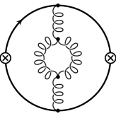
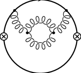
Figure 2: Double bubble diagrams, where the massive quark-antiquark pair is produced by the external current and the internal bubble is purely gluonic. The ghost diagrams are not depicted explicitly.

can be determined by identifying the corresponding moments in the gluonic (and ghost) vacuum polarization function as defined in Eq. (114),

$$R_{\infty}^{g,\overline{\mbox{\tiny MS}}} = C_{A}\left(-\frac{5}{4}-\frac{3}{8}\xi\right),$$

$$R_{0}^{g,\overline{\mbox{\tiny MS}}} = C_{A}\left(\frac{31}{12}-\frac{3}{4}\xi+\frac{3}{16}\xi^{2}+\left(-\frac{5}{4}-\frac{3}{8}\xi\right)\ln 4\right)\,,$$ (120)

where the gauge parameter $\xi$ is defined via the gluon propagator in lowest order

$$\frac{i}{q^{2}+i\,\epsilon}\,\left(-\,g^{\mu\nu}+\xi\,\frac{q^{\mu}\,q^{\nu}}{q^{2}}\right)\,.$$

Obviously the moments and $r_{\Theta,g}^{(2),\overline{\mbox{\tiny MS}}}$, $\Theta=V,A,S,P$, are not gauge invariant. However, for $\xi=4$ the combination $\alpha_{s}^{2}\,R_{\infty}^{g,\overline{\mbox{\tiny MS}}}/(3\pi)$ coincides with the complete gluonic and ghost ${\cal{O}}(\alpha_{s}^{2})$ contributions to the QCD $\beta$-function, and thus $r_{\Theta,g}^{(2),\overline{\mbox{\tiny MS}}}|_{\xi=4}$ accounts for the leading logarithmic behavior of the sum of all gluonic ${\cal{O}}(\alpha_{s}^{2})$ contributions (i.e. proportional to $C_{A}C_{F}$) in the high energy limit. It is quite trivial that such a $\xi$ can be found, but it is a remarkable fact that even in the non-relativistic limit, i.e. keeping only the leading terms for $\beta=\sqrt{1-4M^{2}/q^{2}}\to 0$, $r_{\Theta,g}^{(2),\overline{\mbox{\tiny MS}}}|_{\xi=4}$ accounts for all ${\cal{O}}(\alpha_{s}^{2})$ corrections to the rates proportional to the color factors $C_{A}C_{F}$. This issue has already been pointed out in [16] for the vector current induced rate and has been used in [10] for the construction of Padè approximants. In Section 7 we will explicitly demonstrate this fact also for the axial-vector, scalar and pseudoscalar current induced rates.

7 Examining the Region for small $\beta$ – close to Threshold

In the previous sections we have determined the ${\cal{O}}(\alpha_{s}^{2})$ light quark non-singlet corrections to the total heavy quark-antiquark production rates induced by the vector, axial-vector, scalar and pseudoscalar currents for all energies above the heavy quark-antiquark threshold, $q^{2}>4M^{2}$. Using the method of the moments we are further able to calculate the ${\cal{O}}(\alpha_{s}^{2})$ corrections to the rates proportional to the color factors $C_{A}C_{F}$ from the (gauge dependent) gluonic and ghost contributions of the ${\cal{O}}(\alpha_{s})$ corrections to the gluon propagator. Having these two-loop results at one’s disposal it is of special interest to consider the kinematic regime close to the threshold, where $\beta=\sqrt{1-4M^{2}/q^{2}}\ll 1$. Using the expansions for $\beta\to 0$ given in Appendix C, the ${\cal{O}}(\alpha_{s}^{2})$ light quark non-singlet corrections to the rates for all currents read

$$\Big{(}\frac{\alpha_{s}^{\overline{\mbox{\tiny MS}}}(\mu^{2})}{\pi}\Big{)}^{2}\,r^{(2),\overline{\mbox{\tiny MS}}}_{V,q} \stackrel{{\scriptstyle\beta\to 0}}{{=}} N_{c}\,C_{F}\,T\,\Big{(}\frac{\alpha_{s}^{\overline{\mbox{\tiny MS}}}(\mu^{2})}{\pi}\Big{)}^{2}\,\bigg{[}\,\frac{3\,\pi^{2}}{4}\,\bigg{(}\,\frac{1}{3}\,\ln\frac{4\beta^{2}M^{2}}{\mu^{2}}-\frac{5}{9}\,\bigg{)}$$

$$\quad-\,6\,\beta\,\bigg{(}\,\frac{1}{3}\,\ln\frac{M^{2}}{\mu^{2}}-\frac{11}{36}\,\bigg{)}+\frac{\pi^{2}}{2}\,\beta^{2}\,\bigg{(}\,\frac{1}{3}\,\ln\frac{4\beta^{2}M^{2}}{\mu^{2}}-\frac{25}{18}\,\bigg{)}\,\bigg{]}+{\cal{O}}(\beta^{3})\,,$$

$$\Big{(}\frac{\alpha_{s}^{\overline{\mbox{\tiny MS}}}(\mu^{2})}{\pi}\Big{)}^{2}\,r^{(2),\overline{\mbox{\tiny MS}}}_{A,q} \stackrel{{\scriptstyle\beta\to 0}}{{=}} N_{c}\,C_{F}\,T\,\Big{(}\frac{\alpha_{s}^{\overline{\mbox{\tiny MS}}}(\mu^{2})}{\pi}\Big{)}^{2}\,\bigg{[}\,\frac{\pi^{2}}{2}\,\beta^{2}\,\bigg{(}\,\frac{1}{3}\,\ln\frac{4\beta^{2}M^{2}}{\mu^{2}}-\frac{11}{9}\,\bigg{)}$$

$$\quad-\,2\,\beta^{3}\,\bigg{(}\,\frac{1}{3}\,\ln\frac{M^{2}}{\mu^{2}}-\frac{7}{18}\,\bigg{)}+\frac{\pi^{2}}{2}\,\beta^{4}\,\bigg{(}\,\frac{1}{3}\,\ln\frac{4\beta^{2}M^{2}}{\mu^{2}}-\frac{5}{9}\,\bigg{)}\,\bigg{]}+{\cal{O}}(\beta^{5})\,,$$

$$\Big{(}\frac{\alpha_{s}^{\overline{\mbox{\tiny MS}}}(\mu^{2})}{\pi}\Big{)}^{2}\,r^{(2),\overline{\mbox{\tiny MS}}}_{S,q} \stackrel{{\scriptstyle\beta\to 0}}{{=}} N_{c}\,C_{F}\,T\,\Big{(}\frac{\alpha_{s}^{\overline{\mbox{\tiny MS}}}(\mu^{2})}{\pi}\Big{)}^{2}\,\bigg{[}\,\frac{\pi^{2}}{2}\,\beta^{2}\,\bigg{(}\,\frac{1}{3}\,\ln\frac{4\beta^{2}M^{2}}{\mu^{2}}-\frac{11}{9}\,\bigg{)}$$

$$\quad-\,\beta^{3}\,\bigg{(}\,\frac{1}{3}\,\ln\frac{M^{2}}{\mu^{2}}+\frac{5}{18}\,\bigg{)}+\frac{\pi^{2}}{2}\,\beta^{4}\,\bigg{(}\,\frac{1}{3}\,\ln\frac{4\beta^{2}M^{2}}{\mu^{2}}+\frac{4}{9}\,\bigg{)}\,\bigg{]}+{\cal{O}}(\beta^{5})\,,$$

$$\Big{(}\frac{\alpha_{s}^{\overline{\mbox{\tiny MS}}}(\mu^{2})}{\pi}\Big{)}^{2}\,r^{(2),\overline{\mbox{\tiny MS}}}_{P,q} \stackrel{{\scriptstyle\beta\to 0}}{{=}} N_{c}\,C_{F}\,T\,\Big{(}\frac{\alpha_{s}^{\overline{\mbox{\tiny MS}}}(\mu^{2})}{\pi}\Big{)}^{2}\,\bigg{[}\,\frac{\pi^{2}}{2}\,\bigg{(}\,\frac{1}{3}\,\ln\frac{4\beta^{2}M^{2}}{\mu^{2}}-\frac{5}{9}\,\bigg{)}$$

$$\quad-\,3\,\beta\,\bigg{(}\,\frac{1}{3}\,\ln\frac{M^{2}}{\mu^{2}}-\frac{1}{18}\,\bigg{)}+\frac{\pi^{2}}{2}\,\bigg{(}\,\frac{1}{3}\,\ln\frac{4\beta^{2}M^{2}}{\mu^{2}}-\frac{2}{9}\,\bigg{)}\,\beta^{2}\,\bigg{]}+{\cal{O}}(\beta^{3})\,,$$

where we have displayed an expansion up to next-to-next-to-leading order in $\beta$. The corresponding ${\cal{O}}(\alpha_{s}^{2})$ contributions from the gluon propagator corrections are straightforward using the gluonic moments given in Section 6.2. We would like to emphasize that the expansions (7)–(7) have to be considered strictly in the context of fixed order multi-loop perturbation theory which represents primarily an expansion in the strong coupling $\alpha_{s}$. Therefore, the expressions (7)–(7) actually are only good approximations in the kinematic regime where $\alpha_{s}\mathrel{\raise 1.29167pt\hbox{$<$\kern-7.5pt\lower 4.30554pt\hbox{$\sim$}}}\beta\ll 1$. It is evident that this kinematic regime is rather small, in particular for the $c\bar{c}$ and and the $b\bar{b}$ thresholds, where the strong coupling becomes quite large. Nevertheless, it is very instructive to examine the expansions because they allow for some insights into the long- and short-distance structure of the ${\cal{O}}(\alpha_{s}^{2})$ light quark contributions to the rates.

Let us start by comparing the expansions (7)–(7) with the expressions of the ${\cal{O}}(\alpha_{s})$ corrections in the same limit,

$$\Big{(}\frac{\alpha_{s}^{\overline{\mbox{\tiny MS}}}(\mu^{2})}{\pi}\Big{)}\,r^{(1)}_{V} \stackrel{{\scriptstyle\beta\to 0}}{{=}} N_{c}\,C_{F}\,\alpha_{s}^{\overline{\mbox{\tiny MS}}}(\mu^{2})\,\bigg{[}\,\frac{3\,\pi}{4}-\frac{6}{\pi}\,\beta+\frac{\pi}{2}\,\beta^{2}+{\cal{O}}(\beta^{3})\,\bigg{]}\,,$$ (125)

$$\Big{(}\frac{\alpha_{s}^{\overline{\mbox{\tiny MS}}}(\mu^{2})}{\pi}\Big{)}\,r^{(1)}_{A} \stackrel{{\scriptstyle\beta\to 0}}{{=}} N_{c}\,C_{F}\,\alpha_{s}^{\overline{\mbox{\tiny MS}}}(\mu^{2})\,\bigg{[}\,\frac{\pi}{2}\,\beta^{2}-\frac{2}{\pi}\,\beta^{3}+\frac{\pi}{2}\,\beta^{4}+{\cal{O}}(\beta^{5})\,\bigg{]}\,,$$ (126)

$$\Big{(}\frac{\alpha_{s}^{\overline{\mbox{\tiny MS}}}(\mu^{2})}{\pi}\Big{)}\,r^{(1)}_{S} \stackrel{{\scriptstyle\beta\to 0}}{{=}} N_{c}\,C_{F}\,\alpha_{s}^{\overline{\mbox{\tiny MS}}}(\mu^{2})\,\bigg{[}\,\frac{\pi}{2}\,\beta^{2}-\frac{1}{\pi}\,\beta^{3}+\frac{\pi}{2}\,\beta^{4}+{\cal{O}}(\beta^{5})\,\bigg{]}\,,$$ (127)

$$\Big{(}\frac{\alpha_{s}^{\overline{\mbox{\tiny MS}}}(\mu^{2})}{\pi}\Big{)}\,r^{(1)}_{P} \stackrel{{\scriptstyle\beta\to 0}}{{=}} N_{c}\,C_{F}\,\alpha_{s}^{\overline{\mbox{\tiny MS}}}(\mu^{2})\,\bigg{[}\,\frac{\pi}{2}-\frac{3}{\pi}\,\beta+\frac{\pi}{2}\,\beta^{2}+{\cal{O}}(\beta^{3})\,\bigg{]}\,.$$ (128)

Evidently the expansions (7)–(7) can be used to carry out an analysis of the respective BLM scales. This reveals that the leading and next-to-next-to-leading contributions in the small $\beta$-expansion of the ${\cal{O}}(\alpha_{s})$ contributions to the rates are governed by scales of order $2M\beta$, the relative momentum of the produced heavy quark-antiquark pair, indicating that they are of long-distance origin, i.e. generated at non-relativistic momenta. All the next-to-leading contributions for small $\beta$, on the other hand, are governed by a hard scale of the order of the heavy quark mass. This clearly shows that the latter are of short-distance origin, i.e. generated at relativistic momenta. The most striking feature of the expansions (7)–(7), however, is that the leading terms in the small $\beta$-expansion for the vector and pseudoscalar induced rates, on the one hand, and for the axial-vector and scalar current induced rates, on the other, are proportional to each other. Further, the axial-vector and scalar current induced rates are suppressed by $\beta^{2}$ with respect to the vector and pseudoscalar induced rates. For the rest of this section we will concentrate only on these dominant contributions for the expansion in $\beta$. In particular, we will demonstrate explicitly by using non-relativistic considerations that the latter contributions are uniquely determined by the static color potential and the orbital angular momentum states in which the heavy quark-antiquark pair is produced by the currents. Because the static potential and the orbital angular momentum represent all the information needed to completely describe the heavy quark-antiquark pair in the non-relativistic limit, the calculations in the following will also illustrate the fact that for small $\beta$ the ${\cal{O}}(\alpha_{s}^{2})$ light quark corrections from secondary heavy quark production (class(ii)) and the ${\cal{O}}(\alpha_{s}^{2})$ light quark singlet corrections (class(iii)) are suppressed with respect to the non-singlet contributions calculated in this work. Using the same line of reasoning we will also determine the leading ${\cal{O}}(C_{A}C_{F}\alpha_{s}^{2})$ corrections in the non-relativistic limit and demonstrate that they are equal to $r_{\Theta,g}^{(2),\overline{\mbox{\tiny MS}}}|_{\xi=4}$, proving the statement given in Section 6.2.

For illustration let us first discuss the simpler case of the ${\cal{O}}(\alpha_{s})$ corrections to the rates in the non-relativistic limit, Eqs. (125)–(128). The dominant contributions for small $\beta$ can be reproduced by the following consideration: the vector and pseudoscalar currents produce the heavy quark-antiquark pair in a (relative orbital angular momentum) S-wave state, whereas the axial-vector and scalar currents lead to a quark-antiquark pair in a P-wave (see e.g. [23]). Via the optical theorem the vector and pseudoscalar rates are therefore proportional to the absorptive part of the zero-distance S-wave Green function, and the axial-vector and scalar rates are proportional to the absorptive part of the zero-distance P-wave Green function of the non-relativistic Schrödinger equation

$$\bigg{[}\,-\frac{1}{M_{Q}}\vec{\nabla}^{2}_{\vec{x}}+V_{\mbox{\tiny QCD}}(\vec{x})-E\,\bigg{]}\,G_{c}(\vec{x},\vec{y})\,=\,\delta^{(3)}(\vec{x}-\vec{y})\,,$$ (129)

where

$$V_{\mbox{\tiny QCD}}(\vec{x})\,=\,-\,C_{F}\,\frac{\alpha_{s}^{\overline{\mbox{\tiny MS}}}(\mu^{2})}{|{\vec{x}}|}$$ (130)

is the leading order static QCD potential, with the strong coupling fixed at the scale $\mu$ and $E\equiv\sqrt{q^{2}}-2M$ is the energy relative to the threshold point. Because we are only interested in the regime where $\alpha_{s}\mathrel{\raise 1.29167pt\hbox{$<$\kern-7.5pt\lower 4.30554pt\hbox{$\sim$}}}\beta\ll 1$ we can determine $G_{c}$ perturbatively using Rayleigh-Schrödinger time-independent perturbation theory (TIPT) starting from the Green function of the free Schrödinger equation,

$$G^{(0)}(\vec{x},\vec{y})\,=\,\frac{M}{4\,\pi}\,\frac{\exp(i\,M\,\beta\,|{\vec{x}}-{\vec{y}}|)}{|{\vec{x}}-{\vec{y}}|}\,.$$ (131)

For the ${\cal{O}}(\alpha_{s})$ contributions to the rates it is sufficient to use first order TIPT,

$$G_{c}^{(1)}(\vec{x},\vec{y})\,=\,-\,\int\!d^{3}{\vec{z}}\,\,\,G^{(0)}(\vec{x},\vec{z})\,\,V_{\mbox{\tiny QCD}}({\vec{z}})\,\,G^{(0)}(\vec{z},\vec{y})\,.$$ (132)

The S-wave contribution in $G_{c}^{(1)}$ at zero distances is just equal to $G_{c}^{(1)}(\vec{x},\vec{y})|_{|\vec{x}|,|\vec{y}|\to 0}$ and the P-wave contribution at zero-distances reads $[\partial_{x^{i}}\,\partial_{y^{i}}\,G_{c}^{(1)}(\vec{x},\vec{y})]|_{|\vec{x}|,|\vec{y}|\to 0}$, where $\partial_{x^{i}}\equiv\partial/\partial x^{i}$ and summation over the spatial index $i$ is understood. Taking into account the normalization of the rates as defined in Eqs. (6) and (8) one finally arrives at

$$\Big{(}\frac{\alpha_{s}^{\overline{\mbox{\tiny MS}}}(\mu^{2})}{\pi}\Big{)}\,r^{(1),\mbox{\tiny nr}}_{V} = N_{c}\,\frac{6\,\pi}{M^{2}}\,\mbox{Im}\,G_{c}^{(1)}(\vec{x},\vec{y})\bigg{|}_{|\vec{x}|,|\vec{y}|\to 0}\,=\,N_{c}\,C_{F}\,\alpha_{s}^{\overline{\mbox{\tiny MS}}}(\mu^{2})\,\frac{3\,\pi}{4}\,,$$ (133)

$$\Big{(}\frac{\alpha_{s}^{\overline{\mbox{\tiny MS}}}(\mu^{2})}{\pi}\Big{)}\,r^{(1),\mbox{\tiny nr}}_{A} = N_{c}\,\frac{4\,\pi}{M^{4}}\,\mbox{Im}\,\bigg{[}\,\frac{\partial}{\partial x^{i}}\frac{\partial}{\partial y^{i}}G_{c}^{(1)}(\vec{x},\vec{y})\,\bigg{]}\bigg{|}_{|\vec{x}|,|\vec{y}|\to 0}\,=\,N_{c}\,C_{F}\,\alpha_{s}^{\overline{\mbox{\tiny MS}}}(\mu^{2})\,\frac{\pi}{2}\,\beta^{2}\,,$$ (134)

$$\Big{(}\frac{\alpha_{s}^{\overline{\mbox{\tiny MS}}}(\mu^{2})}{\pi}\Big{)}\,r^{(1),\mbox{\tiny nr}}_{S} = N_{c}\,\frac{4\,\pi}{M^{4}}\,\mbox{Im}\,\bigg{[}\,\frac{\partial}{\partial x^{i}}\frac{\partial}{\partial y^{i}}G_{c}^{(1)}(\vec{x},\vec{y})\,\bigg{]}\bigg{|}_{|\vec{x}|,|\vec{y}|\to 0}\,=\,N_{c}\,C_{F}\,\alpha_{s}^{\overline{\mbox{\tiny MS}}}(\mu^{2})\,\frac{\pi}{2}\,\beta^{2}\,,\quad$$ (135)

$$\Big{(}\frac{\alpha_{s}^{\overline{\mbox{\tiny MS}}}(\mu^{2})}{\pi}\Big{)}\,r^{(1),\mbox{\tiny nr}}_{P} = N_{c}\,\frac{4\,\pi}{M^{2}}\,\mbox{Im}\,G_{c}^{(1)}(\vec{x},\vec{y})\bigg{|}_{|\vec{x}|,|\vec{y}|\to 0}\,=\,N_{c}\,C_{F}\,\alpha_{s}^{\overline{\mbox{\tiny MS}}}(\mu^{2})\,\frac{\pi}{2}\,,$$ (136)

which is equivalent to the dominant contributions in Eqs. (125)–(128). Obviously the $\beta^{2}$ suppression of the axial-vector and scalar rates comes from the fact that the latter correspond to heavy quark-antiquark pairs in a P-wave state.

It is now an easy task to determine all ${\cal{O}}(\alpha_{s}^{2})$ corrections to the rates in the non-relativistic limit coming from light quarks by taking into account the radiative corrections to the static QCD potential due to one massless quark species [24] in the configuration space representation [25]

$$\delta V_{\mbox{\tiny QCD},q}(\vec{x}) = -\,C_{F}\,T\,\frac{\alpha_{s}^{\overline{\mbox{\tiny MS}}}(\mu^{2})}{|{\vec{x}}|}\,\frac{2\,\alpha_{s}^{\overline{\mbox{\tiny MS}}}(\mu^{2})}{3\,\pi}\,\bigg{[}\,\ln\frac{1}{\mu\,|\vec{x}|}-\gamma-\frac{5}{6}\,\bigg{]}$$ (137)

$$= -\,C_{F}\,\frac{\alpha_{s}^{\overline{\mbox{\tiny MS}}}(\mu^{2})}{|{\vec{x}}|}\,\frac{2\,\alpha_{s}^{\overline{\mbox{\tiny MS}}}(\mu^{2})}{3\,\pi}\,\bigg{[}\,R_{\infty}^{q,\overline{\mbox{\tiny MS}}}\bigg{(}\,\ln\frac{1}{2\,\mu\,|\vec{x}|}-\gamma\,\bigg{)}+\frac{1}{2}\,R_{0}^{q,\overline{\mbox{\tiny MS}}}\,\bigg{]}\,.$$

Because the corrections to the QCD potential from massless quarks originate completely from the Serber-Uehling light quark vacuum polarization [24], Eq. (114), $\delta V_{\mbox{\tiny QCD},q}$ can be completely expressed in terms of the moments $R_{\infty}^{q,\overline{\mbox{\tiny MS}}}$ and $R_{0}^{q,\overline{\mbox{\tiny MS}}}$. Using the same line of reasoning as presented for the ${\cal{O}}(\alpha_{s})$ contributions to the rates, the ${\cal{O}}(\alpha_{s}^{2})$ light quark corrections in the non-relativistic limit can now be determined by calculating the first order (TIPT) correction to the Green function due to $\delta V_{\mbox{\tiny QCD},q}$,

$$G_{c,q}^{(1)}(\vec{x},\vec{y})\,=\,-\,\int\!d^{3}{\vec{z}}\,\,\,G^{(0)}(\vec{x},\vec{z})\,\,\delta V_{\mbox{\tiny QCD},q}({\vec{z}})\,\,G^{(0)}(\vec{z},\vec{y})\,.$$ (138)

Extracting the zero-distance S- and P-wave contributions in analogy to Eqs. (133)–(136) we arrive at

$$\Big{(}\frac{\alpha_{s}^{\overline{\mbox{\tiny MS}}}(\mu^{2})}{\pi}\Big{)}^{2}\,r^{(2),\mbox{\tiny nr}}_{V,q} = N_{c}\,\frac{6\,\pi}{M^{2}}\,\mbox{Im}\,G_{c,q}^{(1)}(\vec{x},\vec{y})\bigg{|}_{|\vec{x}|,|\vec{y}|\to 0}$$ (139)

$$= N_{c}\,C_{F}\,\Big{(}\alpha_{s}^{\overline{\mbox{\tiny MS}}}(\mu^{2})\Big{)}^{2}\,\frac{1}{4}\,\bigg{[}\,R_{\infty}^{q,\overline{\mbox{\tiny MS}}}\,\ln\frac{\beta^{2}M^{2}}{\mu^{2}}+R_{0}^{q,\overline{\mbox{\tiny MS}}}\,\bigg{]}$$

$$= N_{c}\,C_{F}\,T\,\Big{(}\alpha_{s}^{\overline{\mbox{\tiny MS}}}(\mu^{2})\Big{)}^{2}\,\frac{1}{4}\,\bigg{[}\,\ln\frac{4\beta^{2}M^{2}}{\mu^{2}}-\frac{5}{3}\,\bigg{]}\,,$$

$$\Big{(}\frac{\alpha_{s}^{\overline{\mbox{\tiny MS}}}(\mu^{2})}{\pi}\Big{)}^{2}\,r^{(2),\mbox{\tiny nr}}_{A,q} = N_{c}\,\frac{4\,\pi}{M^{4}}\,\mbox{Im}\,\bigg{[}\,\frac{\partial}{\partial x^{i}}\frac{\partial}{\partial y^{i}}G_{c}^{(1)}(\vec{x},\vec{y})\,\bigg{]}\bigg{|}_{|\vec{x}|,|\vec{y}|\to 0}$$ (140)

$$= N_{c}\,C_{F}\,\Big{(}\alpha_{s}^{\overline{\mbox{\tiny MS}}}(\mu^{2})\Big{)}^{2}\,\frac{1}{6}\,\bigg{[}\,R_{\infty}^{q,\overline{\mbox{\tiny MS}}}\,\bigg{(}\,\ln\frac{\beta^{2}M^{2}}{\mu^{2}}-2\,\bigg{)}+R_{0}^{q,\overline{\mbox{\tiny MS}}}\,\bigg{]}\,\beta^{2}$$

$$= N_{c}\,C_{F}\,T\,\Big{(}\alpha_{s}^{\overline{\mbox{\tiny MS}}}(\mu^{2})\Big{)}^{2}\,\frac{1}{6}\,\bigg{[}\,\ln\frac{4\beta^{2}M^{2}}{\mu^{2}}-\frac{11}{3}\,\bigg{]}\,\beta^{2}\,,$$

$$\Big{(}\frac{\alpha_{s}^{\overline{\mbox{\tiny MS}}}(\mu^{2})}{\pi}\Big{)}^{2}\,r^{(2),\mbox{\tiny nr}}_{S,q} = \Big{(}\frac{\alpha_{s}^{\overline{\mbox{\tiny MS}}}(\mu^{2})}{\pi}\Big{)}^{2}\,r^{(2),\mbox{\tiny nr}}_{A,q}\,,$$ (141)

$$\Big{(}\frac{\alpha_{s}^{\overline{\mbox{\tiny MS}}}(\mu^{2})}{\pi}\Big{)}^{2}\,r^{(2),\mbox{\tiny nr}}_{P,q} = \frac{2}{3}\,\Big{(}\frac{\alpha_{s}^{\overline{\mbox{\tiny MS}}}(\mu^{2})}{\pi}\Big{)}^{2}\,r^{(2),\mbox{\tiny nr}}_{V,q}\,,$$ (142)

which is in agreement with the dominant contributions in Eqs. (7)–(7). This also illustrates the statement that the ${\cal{O}}(\alpha_{s}^{2})$ light quark non-singlet corrections dominate the contributions from classes (ii) and (iii) in the non-relativistic limit. Further, Eqs. (139)–(142) demonstrate explicitly why the vector and pseudoscalar rates, and the axial-vector and scalar rates are proportional to each other in the non-relativistic limit.

In the same manner we can now determine all the ${\cal{O}}(C_{A}C_{F}\alpha_{s}^{2})$ contributions to the rate in the non-relativistic limit by calculating the first order (TIPT) corrections to the Green function due to the gluonic corrections to the QCD potential proportional to $C_{A}C_{F}$ [26],

$$\delta V_{\mbox{\tiny QCD},q}(\vec{x}) = -\,C_{F}\,C_{A}\,\frac{\alpha_{s}^{\overline{\mbox{\tiny MS}}}(\mu^{2})}{|{\vec{x}}|}\,\frac{2\,\alpha_{s}^{\overline{\mbox{\tiny MS}}}(\mu^{2})}{3\,\pi}\,\bigg{[}\,-\frac{11}{4}\,\bigg{(}\,\ln\frac{1}{\mu\,|\vec{x}|}-\gamma\,\bigg{)}+\frac{31}{24}\,\bigg{]}$$ (143)

$$= -\,C_{F}\,\frac{\alpha_{s}^{\overline{\mbox{\tiny MS}}}(\mu^{2})}{|{\vec{x}}|}\,\frac{2\,\alpha_{s}^{\overline{\mbox{\tiny MS}}}(\mu^{2})}{3\,\pi}\,\bigg{[}\,R_{\infty}^{g,\overline{\mbox{\tiny MS}}}\bigg{(}\,\ln\frac{1}{2\,\mu\,|\vec{x}|}-\gamma\,\bigg{)}+\frac{1}{2}\,R_{0}^{g,\overline{\mbox{\tiny MS}}}\,\bigg{]}\,\bigg{|}_{\xi=4}\,.$$

It is a non-trivial fact that the gluonic corrections to the QCD-potential can be expressed entirely in terms of the gluonic and gauge dependent moments $R_{\infty}^{g,\overline{\mbox{\tiny MS}}}$ and $R_{0}^{g,\overline{\mbox{\tiny MS}}}$ for the special choice of the gauge parameter $\xi=4$ because the $C_{A}C_{F}$ corrections to the QCD potential arise from the combination of one-loop propagator corrections, box diagrams and gluonic vertex corrections. As already mentioned in Section 6.2 it is quite trivial that such a value of $\xi$ can be found for the logarithmic contribution in $\delta V_{\mbox{\tiny QCD},q}$, but it is a remarkable fact that also the non-logarithmic term is accounted for completely by $R_{0}^{g,\overline{\mbox{\tiny MS}}}$ for the same value of $\xi$. Proceeding along the lines of the ${\cal{O}}(\alpha_{s}^{2})$ light quark corrections we can now easily determine the ${\cal{O}}(C_{A}C_{F}\alpha_{s}^{2})$ corrections to the rates in the non-relativistic limit,

$$\Big{(}\frac{\alpha_{s}^{\overline{\mbox{\tiny MS}}}(\mu^{2})}{\pi}\Big{)}^{2}\,r^{(2),\mbox{\tiny nr}}_{V,g} = N_{c}\,C_{F}\,\Big{(}\alpha_{s}^{\overline{\mbox{\tiny MS}}}(\mu^{2})\Big{)}^{2}\,\frac{1}{4}\,\bigg{[}\,R_{\infty}^{g,\overline{\mbox{\tiny MS}}}\,\ln\frac{\beta^{2}M^{2}}{\mu^{2}}+R_{0}^{g,\overline{\mbox{\tiny MS}}}\,\bigg{]}\bigg{|}_{\xi=4}$$ (144)

$$= N_{c}\,C_{A}\,C_{F}\,\Big{(}\alpha_{s}^{\overline{\mbox{\tiny MS}}}(\mu^{2})\Big{)}^{2}\,\frac{1}{4}\,\bigg{[}\,-\frac{11}{4}\,\ln\frac{4\beta^{2}M^{2}}{\mu^{2}}+\frac{31}{12}\,\bigg{]}\,,$$

$$\Big{(}\frac{\alpha_{s}^{\overline{\mbox{\tiny MS}}}(\mu^{2})}{\pi}\Big{)}^{2}\,r^{(2),\mbox{\tiny nr}}_{A,g} = N_{c}\,C_{F}\,\Big{(}\alpha_{s}^{\overline{\mbox{\tiny MS}}}(\mu^{2})\Big{)}^{2}\,\frac{1}{6}\,\bigg{[}\,R_{\infty}^{g,\overline{\mbox{\tiny MS}}}\,\bigg{(}\,\ln\frac{\beta^{2}M^{2}}{\mu^{2}}-2\,\bigg{)}+R_{0}^{g,\overline{\mbox{\tiny MS}}}\,\bigg{]}\,\beta^{2}\,\bigg{|}_{\xi=4}$$ (145)

$$= N_{c}\,C_{A}\,C_{F}\,\Big{(}\alpha_{s}^{\overline{\mbox{\tiny MS}}}(\mu^{2})\Big{)}^{2}\,\frac{1}{6}\,\bigg{[}\,-\frac{11}{4}\,\ln\frac{4\beta^{2}M^{2}}{\mu^{2}}+\frac{97}{12}\,\bigg{]}\,\beta^{2}\,,$$

$$\Big{(}\frac{\alpha_{s}^{\overline{\mbox{\tiny MS}}}(\mu^{2})}{\pi}\Big{)}^{2}\,r^{(2),\mbox{\tiny nr}}_{S,g} = \Big{(}\frac{\alpha_{s}^{\overline{\mbox{\tiny MS}}}(\mu^{2})}{\pi}\Big{)}^{2}\,r^{(2),\mbox{\tiny nr}}_{A,g}\,,$$ (146)

$$\Big{(}\frac{\alpha_{s}^{\overline{\mbox{\tiny MS}}}(\mu^{2})}{\pi}\Big{)}^{2}\,r^{(2),\mbox{\tiny nr}}_{P,g} = \frac{2}{3}\,\Big{(}\frac{\alpha_{s}^{\overline{\mbox{\tiny MS}}}(\mu^{2})}{\pi}\Big{)}^{2}\,r^{(2),\mbox{\tiny nr}}_{V,g}\,,$$ (147)

which proves our statement given in Section 6.2.

To conclude, we would like to note that although the results in Eqs. (7)–(7) (and also Eqs. (139)–(142)) are only applicable for $\alpha_{s}\mathrel{\raise 1.29167pt\hbox{$<$\kern-7.5pt\lower 4.30554pt\hbox{$\sim$}}}\beta\ll 1$, they represent very important results for predictions of the rates for $|\beta|\mathrel{\raise 1.29167pt\hbox{$<$\kern-7.5pt\lower 4.30554pt\hbox{$\sim$}}}\alpha_{s}$ because they allow for an extraction of the short distance effects coming from the light quark dynamics. These short-distance effects are universal for $|\beta|\ll 1$, regardless whether $\beta$ is smaller or larger than $\alpha_{s}$. Therefore, in an effective field theory approach like NRQCD [27], results (7)–(7) are an important input for the so called “matching calculations” which allow for a systematic extraction of short-distance contributions. Such a treatment, however, is beyond the scope of this paper and shall be carried out elsewhere.

8 Summary

The non-singlet ${\cal{O}}(\alpha_{s}^{2})$ corrections from light quarks to the rates for primary production of massive quark pairs have been calculated analytically for the production through the vector, axial-vector, scalar and pseudoscalar currents. The results have been expressed in terms of moments of the vacuum polarization from the light quarks which allows for an immediate determination of ${\cal{O}}(\alpha_{s}^{2})$ corrections from light colored scalar particles and from the gluonic vacuum polarization insertion. We have analyzed the results in the kinematic regime close to the massive quark-antiquark threshold and have shown that the dominant contributions in the non-relativistic limit can be reproduced from non-relativistic considerations using only the radiative corrections to the QCD potential and the information on the orbital angular momentum state in which the massive quark pair is produced.

Appendix A First Order Corrections from Virtual and Real Radiation of a Massive Vector Boson

In this appendix we present the ${\cal{O}}(\alpha)$ QED corrections to the heavy quark production vertices from virtual and real radiation of a vector boson of mass $\lambda$. Virtual and real radiation corrections are displayed separately. The virtual corrections are presented in terms of the functions

$$\Phi(\xi)\,\equiv\,\frac{1}{2}\sqrt{\xi^{2}-4\,\xi}\ln\left(\frac{\xi-\sqrt{\xi^{2}-4\,\xi}}{\xi+\sqrt{\xi^{2}-4\,\xi}}\right)\sqrt{4\,\xi-\xi^{2}}\,\arctan\left(\frac{\sqrt{4\,\xi-\xi^{2}}}{\xi}\right)\,,\qquad\xi>0\,,$$ (148)

and

$$\Psi(p,\xi)\,\equiv\,\frac{1}{2}\ln^{2}\left(\frac{1}{2}\left[\xi-2+\sqrt{\xi^{2}-4\,\xi}\right]\right)$$ (152)

$$+\mbox{Li}_{2}\left(1+\frac{p}{2}\left[-2+\xi+\sqrt{\xi^{2}-4\,\xi}\right]\right)+\mbox{Li}_{2}\left(1+\frac{p}{2}\left[-2+\xi-\sqrt{\xi^{2}-4\,\xi}\right]\right)$$

$$+\left\{\begin{array}[]{ll}\displaystyle{-\frac{3}{2}\,\pi^{2}+4\,\pi\arctan\left(\frac{\sqrt{4\,\xi-\xi^{2}}}{\xi}\right)+2\,\pi\arctan\left(\frac{2\,p+\xi-2}{\sqrt{4\,\xi-\xi^{2}}}\right)\,,}&0<\xi<4\\ \displaystyle{-\frac{1}{2}\,\pi^{2}+i\,\pi\,\ln\Big{(}(1-p)^{2}+p\,\xi\Big{)}}\,,&\xi>4\end{array}\right.\,,$$

whereas the real corrections are expressed in terms of an one-dimensional integral representation. The parameter $\ell$ is defined as

$$\ell\,\equiv\,\frac{\lambda^{2}}{M^{2}}\,,$$

and

$$\beta\,=\,\sqrt{1-\frac{4\,M^{2}}{q^{2}}}\,,\qquad p\,=\,\frac{1-\beta}{1+\beta}\,.$$

The real parts of the vector current form factors $F_{1/2}^{(1)}$ have already been given in [14, 18].

A.1 Vector Current Vertex

$$F_{1}^{(1)}(M^{2},q^{2},\lambda^{2})\,=\,-\frac{1}{4\,\beta}\,\bigg{[}\,1+{{\beta}^{2}}+\frac{1-{{\beta}^{2}}}{{{\beta}^{2}}}\,\ell\,\bigg{(}1+\frac{\left(3-2\,{{\beta}^{2}}\right)\,\left(1-{{\beta}^{2}}\right)}{8\,{{\beta}^{2}}}\,\ell\bigg{)}\ \,\bigg{]}\,\Psi(p,\ell)\,$$ (153)

$$\mbox{}+\bigg{[}\,\frac{-1+2\,{{\beta}^{2}}}{2\,{{\beta}^{2}}}+\frac{-3+7\,{{\beta}^{2}}+2\,{{\beta}^{4}}}{8\,{{\beta}^{4}}}\,\ell+\frac{3}{\ell-4}\,\bigg{]}\,\Phi(\ell)\,\,$$

$$\mbox{}+\frac{1}{16\,{{\beta}^{4}}}\,\bigg{[}\,-3+7\,{{\beta}^{2}}+2\,{{\beta}^{4}}+\frac{{{\left(1-{{\beta}^{2}}\right)}^{2}}\,\left(-3+2\,{{\beta}^{2}}\right)}{2\,\beta}\,\ln p\,\bigg{]}\,{{\ell}^{2}}\,\ln\ell\,\,$$

$$\mbox{}-\frac{1}{2\,{{\beta}^{2}}}\,\bigg{[}\,1+\frac{1-{{\beta}^{2}}}{2\,\beta}\,\ln p\,\bigg{]}\,\ell\,\ln\ell-\bigg{[}\,\frac{1}{2}+\frac{1+{{\beta}^{2}}}{4\,\beta}\,\ln p\,\bigg{]}\,\ln\ell\,\,$$

$$\mbox{}+\bigg{[}\,\frac{{{\left(1-{{\beta}^{2}}\right)}^{2}}\,\left(-3+2\,{{\beta}^{2}}\right)}{64\,{{\beta}^{5}}}\,\ln^{2}p\,\bigg{]}\,\ell^{2}\,\,$$

$$\mbox{}+\frac{1}{4\,{{\beta}^{2}}}\,\bigg{[}\,-\left(1+2\,{{\beta}^{2}}\right)+\frac{1-{{\beta}^{2}}}{2\,\beta}\,\ln p\,\left(-3+2\,{{\beta}^{2}}-\ln p\right)\,\bigg{]}\,\ell\,\,$$

$$\mbox{}-\frac{1}{8\,\beta}\,\ln p\,\bigg{(}2\,\left(1+2\,{{\beta}^{2}}\right)+\left(1+{{\beta}^{2}}\right)\,\ln p\bigg{)}-1\,\,$$

$$\mbox{}+i\,\pi\,\left\{-\frac{1+2\,{{\beta}^{2}}}{4\,\beta}+\frac{\left(1-{{\beta}^{2}}\right)\,\left(-3+2\,{{\beta}^{2}}\right)}{8\,{{\beta}^{3}}}\,\ell\,\right.\,\,$$

$$\mbox{}\,\qquad\,\left.+\frac{1}{4\,\beta}\,\bigg{[}\,1+{{\beta}^{2}}+\frac{1-{{\beta}^{2}}}{{{\beta}^{2}}}\,\ell+\frac{\left(3-2\,{{\beta}^{2}}\right)\,{{\left(1-{{\beta}^{2}}\right)}^{2}}}{8\,{{\beta}^{4}}}\,\ell^{2}\,\bigg{]}\,\ln(1+\frac{{{\left(1-p\right)}^{2}}}{\ell\,p})\right\}\,,$$

$$F_{2}^{(1)}(M^{2},q^{2},\lambda^{2})\,=\,\frac{{{\left(1-{{\beta}^{2}}\right)}^{2}}}{4\,{{\beta}^{3}}}\,\bigg{[}\,1+\frac{3\,\left(1-{{\beta}^{2}}\right)}{8\,{{\beta}^{2}}}\,\ell\,\bigg{]}\,\ell\,\Psi(p,\ell)+\frac{1-{{\beta}^{2}}}{2\,{{\beta}^{2}}}\,\bigg{[}\,1+\frac{3-5\,{{\beta}^{2}}}{4\,{{\beta}^{2}}}\,\ell\,\bigg{]}\,\Phi(\ell)\,$$ (154)

$$\mbox{}+\frac{{{\left(1+\beta\right)}^{2}}\,\left(1-{{\beta}^{2}}\right)}{16\,{{\beta}^{4}}}\,\bigg{[}\,\frac{3-5\,{{\beta}^{2}}}{{{\left(1+\beta\right)}^{2}}}+\frac{3\,{{\left(1-\beta\right)}^{2}}}{2\,\beta}\,\ln p\,\bigg{]}\,{{\ell}^{2}}\,\ln\ell\,\,$$

$$\mbox{}+\frac{1-{{\beta}^{2}}}{2\,{{\beta}^{2}}}\,\bigg{[}\,1+\frac{1-{{\beta}^{2}}}{2\,\beta}\,\ln p\,\bigg{]}\,\ell\,\ln\ell+\frac{3\,{{\left(1-{{\beta}^{2}}\right)}^{3}}}{64\,{{\beta}^{5}}}\,\bigg{[}\,\ln^{2}p\,\bigg{]}\,{{\ell}^{2}}\,\,$$

$$\mbox{}+\frac{1-{{\beta}^{2}}}{4\,{{\beta}^{2}}}\,\bigg{[}\,1+\frac{1-{{\beta}^{2}}}{2\,\beta}\,\ln p\,\left(3+\ln p\right)\,\bigg{]}\,\ell+\frac{1-{{\beta}^{2}}}{4\,\beta}\,\ln p\,\,$$

$$\mbox{}+i\,\pi\,\left\{\,\frac{1-{{\beta}^{2}}}{4\,\beta}+\frac{3\,{{\left(1-{{\beta}^{2}}\right)}^{2}}}{8\,{{\beta}^{3}}}\,\ell\,\right.\,\,$$

$$\mbox{}\,\qquad\,\left.-\frac{{{\left(1-{{\beta}^{2}}\right)}^{2}}}{4\,{{\beta}^{3}}}\,\bigg{[}\,1+\frac{3\,\left(1-{{\beta}^{2}}\right)}{8\,{{\beta}^{2}}}\,\ell\,\bigg{]}\,\ell\,\ln(1+\frac{{{\left(1-p\right)}^{2}}}{\ell\,p})\,\right\}\,,$$

$$r_{V}^{(1),real}(M^{2},q^{2},\lambda^{2})\,=\,$$ (155)

$$\int_{4M^{2}/q^{2}}^{(1-\sqrt{z})^{2}}{\rm d}y\,\Bigg{\{}-\sqrt{1-\frac{4M^{2}}{q^{2}y}}\,\Lambda^{1/2}(y,z)\,\Bigg{[}1+\Bigg{(}\frac{16M^{4}}{q^{4}}+\frac{8M^{2}}{q^{2}}+4\bigg{(}1+\frac{2M^{2}}{q^{2}}\bigg{)}z\,\Bigg{)}\,D\,\Bigg{]}$$

$$\mbox{}\qquad\qquad\qquad+\bigg{[}\frac{8M^{4}}{q^{4}}+\frac{4M^{2}}{q^{2}}(1-y+z)-(1-y+z)^{2}-2(1+z)y\,\bigg{]}\,L\,\Bigg{\}}\,,$$

where

$$z = \frac{\lambda^{2}}{q^{2}}$$ (156)

$$L \equiv \frac{1}{1-y+z}\,\ln\frac{1-y+z-\sqrt{1-\frac{4M^{2}}{q^{2}y}}\,\Lambda^{1/2}(y,z)}{1-y+z+\sqrt{1-\frac{4M^{2}}{q^{2}y}}\,\Lambda^{1/2}(y,z)}\,,$$ (157)

$$D \equiv \bigg{[}(1-y+z)^{2}-\bigg{(}1-\frac{4M^{2}}{q^{2}y}\bigg{)}\,\Lambda(y,z)\,\bigg{]}^{-1}\,,$$ (158)

$$\Lambda(y,z) \equiv 1+y^{2}+z^{2}-2(y+z+yz)\,.$$ (159)

A.2 Axial-Vector Current Vertex

$$F_{3}^{(1)}(M^{2},q^{2},\lambda^{2})\,=\,-\frac{1+{{\beta}^{2}}}{4\,\beta}\,\bigg{[}\,1+\frac{1-{{\beta}^{2}}}{2\,{{\beta}^{2}}}\,\ell\,\bigg{(}1+\frac{1-{{\beta}^{2}}}{4\,\left(1+{{\beta}^{2}}\right)}\,\ell\bigg{)}\,\bigg{]}\,\Psi(p,\ell)\,$$ (160)

$$\mbox{}-\bigg{[}\,\frac{1-2\,{{\beta}^{2}}}{2\,{{\beta}^{2}}}+\frac{1-7\,{{\beta}^{2}}}{8\,{{\beta}^{2}}}\,\ell-\frac{3}{\ell-4}\,\bigg{]}\,\Phi(\ell)\,\,$$

$$\mbox{}-\frac{1}{16\,{{\beta}^{2}}}\,\bigg{[}\,1-7\,{{\beta}^{2}}+\frac{{{\left(1-{{\beta}^{2}}\right)}^{2}}}{2\,\beta}\,\ln p\,\bigg{]}\,{{\ell}^{2}}\,\ln\ell\,\,$$

$$\mbox{}-\frac{1+{{\beta}^{2}}}{4\,{{\beta}^{2}}}\,\bigg{[}\,1+\frac{1-{{\beta}^{2}}}{2\,\beta}\,\ln p\,\bigg{]}\,\ell\,\ln\ell-\frac{1}{2}\,\bigg{[}\,1+\frac{1+{{\beta}^{2}}}{2\,\beta}\,\ln p\,\bigg{]}\,\ln\ell\,\,$$

$$\mbox{}-\frac{{{\left(1-{{\beta}^{2}}\right)}^{2}}}{64\,{{\beta}^{3}}}\,\bigg{[}\,\ln^{2}p\,\bigg{]}\,\ell^{2}-\frac{1}{4}\,\bigg{[}\,3+\frac{1-{{\beta}^{2}}}{2\,\beta}\,\ln p+\frac{1-{{\beta}^{4}}}{4\,{{\beta}^{3}}}\,\ln^{2}p\,\bigg{]}\,\ell\,\,$$

$$\mbox{}-\frac{1}{4\,\beta}\,\bigg{[}\,2+{{\beta}^{2}}+\frac{1+{{\beta}^{2}}}{2}\,\ln p\,\bigg{]}\,\ln p-1\,\,$$

$$\mbox{}+i\,\pi\,\left\{\,-\frac{2+{{\beta}^{2}}}{4\,\beta}-\frac{1-{{\beta}^{2}}}{8\,\beta}\,\ell\,\right.\,\,$$

$$\mbox{}\,\qquad\,\left.+\frac{1}{4\,\beta}\,\bigg{[}\,1+{{\beta}^{2}}+\frac{1-{{\beta}^{4}}}{2\,{{\beta}^{2}}}\,\ell+\frac{{{\left(1-{{\beta}^{2}}\right)}^{2}}}{8\,{{\beta}^{2}}}\,{{\ell}^{2}}\,\bigg{]}\,\ln(1+\frac{{{\left(1-p\right)}^{2}}}{\ell\,p})\,\right\}\,,$$

$$F_{4}^{(1)}(M^{2},q^{2},\lambda^{2})\,=\,-\frac{{{\left(1-{{\beta}^{2}}\right)}^{2}}}{8\,{{\beta}^{3}}}\,\bigg{[}\,1+{{\beta}^{2}}+\frac{1-{{\beta}^{2}}}{4}\,\ell\,\bigg{]}\,\ell\,\Psi(p,\ell)$$ (161)

$$-\frac{1-{{\beta}^{2}}}{8\,{{\beta}^{2}}}\,\bigg{[}\,4+\left(1+{{\beta}^{2}}\right)\,\ell\,\bigg{]}\,\Phi(\ell)\,-\frac{1-{{\beta}^{2}}}{16\,{{\beta}^{2}}}\,\bigg{[}\,1+{{\beta}^{2}}+\frac{{{\left(1-{{\beta}^{2}}\right)}^{2}}}{2\,\beta}\,\ln p\,\bigg{]}\,{{\ell}^{2}}\,\ln\ell\,\,$$

$$\mbox{}-\frac{{{\left(1-{{\beta}^{2}}\right)}^{2}}}{4\,{{\beta}^{2}}}\,\bigg{[}\,1+\frac{1+{{\beta}^{2}}}{2\,\beta}\,\ln p\,\bigg{]}\,\ell\,\ln\ell-\frac{{{\left(1-{{\beta}^{2}}\right)}^{3}}}{64\,{{\beta}^{3}}}\,\bigg{[}\,\ln^{2}p\,\bigg{]}\,{{\ell}^{2}}\,\,$$

$$\mbox{}+\frac{1-{{\beta}^{2}}}{4}\,\bigg{[}\,1-\frac{1-{{\beta}^{2}}}{2\,\beta}\,\ln p-\frac{1-{{\beta}^{4}}}{4\,{{\beta}^{3}}}\,\ln^{2}p\,\bigg{]}\,\ell-\frac{1-{{\beta}^{2}}}{2}\,\bigg{[}\,1+\frac{2+{{\beta}^{2}}}{2\,\beta}\,\ln p\,\bigg{]}\,\,$$

$$\mbox{}+i\,\pi\,\left\{\,-\frac{\left(1-{{\beta}^{2}}\right)\,\left(2+{{\beta}^{2}}\right)}{4\,\beta}-\frac{{{\left(1-{{\beta}^{2}}\right)}^{2}}}{8\,\beta}\,\ell\,\right.\,\,$$

$$\mbox{}\,\qquad\,\left.+\frac{{{\left(1-{{\beta}^{2}}\right)}^{2}}}{8\,{{\beta}^{3}}}\,\bigg{[}\,1+{{\beta}^{2}}+\frac{1-{{\beta}^{2}}}{4}\,\ell\,\bigg{]}\,\ell\,\ln(1+\frac{{{\left(1-p\right)}^{2}}}{\ell\,p})\,\right\}\,,$$

$$r_{A}^{(1),real}(M^{2},q^{2},\lambda^{2})\,=\,$$ (162)

$$\int_{4M^{2}/q^{2}}^{(1-\sqrt{z})^{2}}{\rm d}y\,\Bigg{\{}-\sqrt{1-\frac{4M^{2}}{q^{2}y}}\,\Lambda^{1/2}(y,z)\,\Bigg{[}1-\Bigg{(}\frac{32M^{4}}{q^{4}}-\frac{8M^{2}}{q^{2}}-4\bigg{(}1-\frac{4M^{2}}{q^{2}}\bigg{)}z\,\Bigg{)}\,D\,\Bigg{]}$$

$$\mbox{}\quad+\bigg{[}-\frac{16M^{4}}{q^{4}}+\frac{4M^{2}}{q^{2}}(1+2y)-\bigg{(}1+\frac{2M^{2}}{q^{2}}\bigg{)}(1-y+z)^{2}-2(1+z)y\,\bigg{]}\,L\,\Bigg{\}}\,,$$

where the functions $L$ and $D$ are given in Eqs. (157) and (158).

A.3 Scalar Current Vertex

$$S^{(1)}(M^{2},q^{2},\lambda^{2})\,=\,-\frac{1}{4\,\beta}\,\bigg{[}\,1+{{\beta}^{2}}+\frac{{{\left(1-{{\beta}^{2}}\right)}^{2}}}{2\,{{\beta}^{2}}}\,\ell\,\bigg{]}\,\Psi(p,\ell)-\bigg{[}\,\frac{1-3\,{{\beta}^{2}}}{2\,{{\beta}^{2}}}-\ell-\frac{3}{\ell-4}\,\bigg{]}\,\Phi(\ell)\,$$ (163)

$$\mbox{}+\frac{1}{2}\,{{\ell}^{2}}\,\ln\ell-\bigg{[}\,\frac{1}{2}+\frac{1+{{\beta}^{2}}}{4\,{{\beta}^{2}}}\,\ell+\frac{1}{4\,\beta}\,\bigg{(}1+{{\beta}^{2}}+\frac{{{\left(1-{{\beta}^{2}}\right)}^{2}}}{2\,{{\beta}^{2}}}\,\ell\bigg{)}\,\ln p\,\bigg{]}\,\ln\ell\,\,$$

$$\mbox{}-\ell-\frac{1}{8\,\beta}\,\bigg{[}\,1+{{\beta}^{2}}+\frac{{{\left(1-{{\beta}^{2}}\right)}^{2}}}{2\,{{\beta}^{2}}}\,\ell\,\bigg{]}\,\ln^{2}p-\frac{1-{{\beta}^{2}}}{2\,\beta}\,\ln p-\frac{1}{2}\,\,$$

$$\mbox{}+i\,\pi\,\left\{\,-\frac{1-{{\beta}^{2}}}{2\,\beta}+\frac{1}{4\,\beta}\,\bigg{[}\,1+{{\beta}^{2}}+\frac{{{\left(1-{{\beta}^{2}}\right)}^{2}}}{2\,{{\beta}^{2}}}\,\ell\,\bigg{]}\,\ln(1+\frac{{{\left(1-p\right)}^{2}}}{\ell\,p})\,\right\}\,,$$

$$r_{S}^{(1),real}(M^{2},q^{2},\lambda^{2})\,=\,$$ (164)

$$\int_{4M^{2}/q^{2}}^{(1-\sqrt{z})^{2}}{\rm d}y\,\Bigg{\{}\sqrt{1-\frac{4M^{2}}{q^{2}y}}\,\Lambda^{1/2}(y,z)\,\bigg{[}\frac{32M^{4}}{q^{4}}-\frac{8M^{2}}{q^{2}}-4\bigg{(}1-\frac{4M^{2}}{q^{2}}\bigg{)}z\,\bigg{]}\,D$$

$$\mbox{}\qquad\qquad\qquad+\bigg{[}-\frac{16M^{4}}{q^{4}}+\frac{4M^{2}}{q^{2}}(1+2y-4z)-1-(z-y)^{2}\,\bigg{]}\,L\,\Bigg{\}}\,.$$

A.4 Pseudoscalar Current Vertex

$$P^{(1)}(M^{2},q^{2},\lambda^{2})\,=\,-\frac{1+{{\beta}^{2}}}{4\,\beta}\,\Psi(p,\ell)+\bigg{[}\,1+\ell+\frac{3}{\ell-4}\,\bigg{]}\,\Phi(\ell)\,$$ (165)

$$\mbox{}-\frac{1}{2}\,\ell\,\left(1-\ell\right)\,\ln\ell-\frac{1}{2}\,\bigg{[}\,1+\frac{1+{{\beta}^{2}}}{2\,\beta}\,\ln p\,\bigg{]}\,\ln\ell-\ell-\frac{1+{{\beta}^{2}}}{8\,\beta}\,\ln^{2}p-\frac{1}{2}\,\,$$

$$\mbox{}+i\,\pi\,\left\{\,\frac{1+{{\beta}^{2}}}{4\,\beta}\,\ln(1+\frac{{{\left(1-p\right)}^{2}}}{\ell\,p})\,\right\}\,,$$

$$r_{P}^{(1),real}(M^{2},q^{2},\lambda^{2})\,=\,$$ (166)

$$\int_{4M^{2}/q^{2}}^{(1-\sqrt{z})^{2}}{\rm d}y\,\Bigg{\{}-4\sqrt{1-\frac{4M^{2}}{q^{2}y}}\,\Lambda^{1/2}(y,z)\,\bigg{(}z+\frac{2M^{2}}{q^{2}}\bigg{)}\,D$$

$$\mbox{}\qquad\qquad\qquad+\bigg{[}\frac{4M^{2}}{q^{2}}-1-(z-y)^{2}\,\bigg{]}\,L\,\Bigg{\}}\,.$$

Appendix B Second Order Corrections from Virtual Massive Quarks

The main focus of this paper is the presentation and discussion of the effects of light quark vacuum polarization insertions into the gluon exchange diagrams for massive quark-antiquark production. This is not an easy task because for the mass assignment $m\ll M$ infrared singularities in the form of logarithms of the ratio $m^{2}/q^{2}$ have to be handled. For the mass constellation $m=M$, however, it has been observed in [14] that the integrations in Eq. (17) become trivial because the square root connected with the born cross-section $\tilde{R}_{q\bar{q}}$ can be substituted away. The results can then be expressed entirely in terms of logarithms. In this appendix we present the results for the axial-vector and pseudoscalar second order form factors for the massive quark pair production vertices coming from the the massive quark-antiquark vacuum polarization insertion into the gluon line, i.e. for $m=M$. For completeness and convenience of the reader we also review the older results for the real parts of the vector and scalar form factors of [14] and [15]. All the imaginary parts of the form factors are new and have to our knowledge never been presented in the literature before. For simplicity all formulae in this appendix are presented in the framework of on-shell QED.

B.1 Vector Current Vertex

$$F_{1,Q}^{(2)} = \frac{1}{12\,{{\beta}^{2}}}\,\bigg{[}\,-\frac{\left(1-2\,{{\beta}^{2}}\right)\,\left(9-6\,{{\beta}^{2}}+5\,{{\beta}^{4}}\right)}{24\,{{\beta}^{3}}}\,\ln^{3}p+\frac{31-23\,{{\beta}^{2}}+30\,{{\beta}^{4}}}{12\,{{\beta}^{2}}}\,\ln^{2}p\,\,$$ (167)

$$\mbox{}\,\qquad+\bigg{(}\frac{267-238\,{{\beta}^{2}}+236\,{{\beta}^{4}}}{18\,\beta}+\frac{\left(1-2\,{{\beta}^{2}}\right)\,\left(9-6\,{{\beta}^{2}}+5\,{{\beta}^{4}}\right)}{2\,{{\beta}^{3}}}\,\zeta(2)\bigg{)}\,\ln p\,\,$$

$$\mbox{}\,+\frac{9-21\,{{\beta}^{2}}-10\,{{\beta}^{4}}}{{{\beta}^{2}}}\,\zeta(2)+\frac{147+236\,{{\beta}^{2}}}{9}\,\bigg{]}\,\,$$

$$\mbox{}\,+i\,\frac{\pi}{16\,{{\beta}^{3}}}\,\bigg{\{}\,-\frac{\left(1-2\,{{\beta}^{2}}\right)\,\left(9-6\,{{\beta}^{2}}+5\,{{\beta}^{4}}\right)}{6\,{{\beta}^{2}}}\,\ln^{2}p+\frac{2\,\left(31-23\,{{\beta}^{2}}+30\,{{\beta}^{4}}\right)}{9\,\beta}\,\ln p\,\,$$

$$\mbox{}\,\qquad+\frac{2\,\left(267-238\,{{\beta}^{2}}+236\,{{\beta}^{4}}\right)}{27}\ \,\bigg{\}}\,,$$

$$F_{2,Q}^{(2)} = \frac{1-{{\beta}^{2}}}{4\,{{\beta}^{2}}}\,\bigg{[}\,\frac{{{\left(1-{{\beta}^{2}}\right)}^{2}}}{8\,{{\beta}^{3}}}\,\ln^{3}p-\frac{11-9\,{{\beta}^{2}}}{12\,{{\beta}^{2}}}\,\ln^{2}p\,\,$$ (168)

$$\mbox{}\,-\bigg{(}\frac{93-68\,{{\beta}^{2}}}{18\,\beta}+\frac{3\,{{\left(1-{{\beta}^{2}}\right)}^{2}}}{2\,{{\beta}^{3}}}\,\zeta(2)\bigg{)}\,\ln p-\frac{3-5\,{{\beta}^{2}}}{{{\beta}^{2}}}\,\zeta(2)-\frac{17}{3}\,\bigg{]}\,\,$$

$$\mbox{}+i\,\pi\,\frac{1-{{\beta}^{2}}}{{{\beta}^{3}}}\,\bigg{\{}\,\frac{3\,{{\left(1-{{\beta}^{2}}\right)}^{2}}}{32\,{{\beta}^{2}}}\,\ln^{2}p-\frac{11-9\,{{\beta}^{2}}}{24\,\beta}\,\ln p-\frac{93-68\,{{\beta}^{2}}}{72}\,\bigg{\}}\,.$$

B.2 Axial-Vector Current Vertex

$$F_{3,Q}^{(2)} = \frac{1}{12\,{{\beta}^{2}}}\,\bigg{[}\,-\frac{3-10\,{{\beta}^{2}}-{{\beta}^{4}}}{24\,\beta}\,\ln^{3}p+\frac{10+25\,{{\beta}^{2}}+3\,{{\beta}^{4}}}{12\,{{\beta}^{2}}}\,\ln^{2}p\,\,$$ (169)

$$\mbox{}+\bigg{(}\frac{60+197\,{{\beta}^{2}}+8\,{{\beta}^{4}}}{18\,\beta}+\frac{3-10\,{{\beta}^{2}}-{{\beta}^{4}}}{2\,\beta}\,\zeta(2)\bigg{)}\,\ln p\,\,$$

$$\mbox{}\,+(3-25\,{{\beta}^{2}})\,\zeta(2)+\frac{30+353\,{{\beta}^{2}}}{9}\,\bigg{]}\,\,$$

$$\mbox{}+i\,\frac{\pi}{24\,{{\beta}^{3}}}\,\bigg{\{}\,-\frac{3-10\,{{\beta}^{2}}-{{\beta}^{4}}}{4}\,\ln^{2}p+\frac{10+25\,{{\beta}^{2}}+3\,{{\beta}^{4}}}{3\,\beta}\,\ln p\,\,$$

$$\mbox{}\,\qquad+\frac{60+197\,{{\beta}^{2}}+8\,{{\beta}^{4}}}{9}\,\bigg{\}}\,,$$

$$F_{4,Q}^{(2)} = \frac{1-{{\beta}^{2}}}{{{\beta}^{2}}}\,\bigg{[}\,-\frac{{{\left(1-{{\beta}^{2}}\right)}^{2}}}{96\,\beta}\,\ln^{3}p+\frac{4+5\,{{\beta}^{2}}-3\,{{\beta}^{4}}}{48\,{{\beta}^{2}}}\,\ln^{2}p\,\,$$ (170)

$$\mbox{}+\bigg{(}\frac{24+47\,{{\beta}^{2}}-20\,{{\beta}^{4}}}{72\,\beta}+\frac{{{\left(1-{{\beta}^{2}}\right)}^{2}}}{8\,\beta}\,\zeta(2)\bigg{)}\,\ln p\,\,$$

$$\mbox{}\,+\frac{1+{{\beta}^{2}}}{4}\,\zeta(2)+\frac{3-5\,{{\beta}^{2}}}{9}\,\bigg{]}\,\,$$

$$\mbox{}+i\,\pi\,\frac{1-{{\beta}^{2}}}{8\,{{\beta}^{3}}}\,\bigg{\{}\,-\frac{{{\left(1-{{\beta}^{2}}\right)}^{2}}}{4}\,\ln^{2}p+\frac{4+5\,{{\beta}^{2}}-3\,{{\beta}^{4}}}{3\,\beta}\,\ln p\,\,$$

$$\mbox{}\,\qquad+\frac{24+47\,{{\beta}^{2}}-20\,{{\beta}^{4}}}{9}\,\bigg{\}}\,.$$

B.3 Scalar Current Vertex

$$S_{Q}^{(2)} = \frac{1+{{\beta}^{2}}}{72\,\beta}\,\ln^{3}p+\frac{5-{{\beta}^{2}}+6\,{{\beta}^{4}}}{72\,{{\beta}^{4}}}\,\ln^{2}p+\bigg{(}\frac{15+2\,{{\beta}^{2}}+11\,{{\beta}^{4}}}{54\,{{\beta}^{3}}}-\frac{1+{{\beta}^{2}}}{6\,\beta}\,\zeta(2)\bigg{)}\,\ln p\,\,$$ (171)

$$\mbox{}\,\quad-\frac{7}{3}\,\zeta(2)+\frac{30+377\,{{\beta}^{2}}}{108\,{{\beta}^{2}}}\,\,$$

$$\mbox{}+i\,\frac{\pi}{6\,\beta}\,\bigg{\{}\,\frac{1+{{\beta}^{2}}}{4}\,\ln^{2}p+\frac{5-{{\beta}^{2}}+6\,{{\beta}^{4}}}{6\,{{\beta}^{3}}}\,\ln p+\frac{15+2\,{{\beta}^{2}}+11\,{{\beta}^{4}}}{9\,{{\beta}^{2}}}\,\bigg{\}}$$

B.4 Pseudoscalar Current Vertex

$$P_{Q}^{(2)} = \frac{1+{{\beta}^{2}}}{6\,\beta}\,\bigg{[}\,\frac{1}{12}\,\ln^{3}p-\frac{1-6\,{{\beta}^{2}}}{12\,{{\beta}^{3}}}\,\ln^{2}p-\bigg{(}\frac{3-17\,{{\beta}^{2}}}{9\,{{\beta}^{2}}}+\zeta(2)\bigg{)}\,\ln p\,\bigg{]}\,\,$$ (172)

$$\mbox{}\,\quad-\frac{7}{3}\,\zeta(2)-\frac{6-413\,{{\beta}^{2}}}{108\,{{\beta}^{2}}}\,\,$$

$$\mbox{}+i\,\pi\,\frac{1+{{\beta}^{2}}}{6\,\beta}\,\bigg{\{}\,\frac{1}{4}\,\ln^{2}p-\frac{1-6\,{{\beta}^{2}}}{6\,{{\beta}^{3}}}\,\ln p-\frac{3-17\,{{\beta}^{2}}}{9\,{{\beta}^{2}}}\,\bigg{\}}$$

Appendix C Expansions

Below we list the expansions of the quantities $\tilde{r}^{(0,1)}_{\Theta}$ and $\delta^{(2)}_{\Theta}$, $\Theta=V,A,S,P$, for energies close to the heavy quark-antiquark production threshold, $\beta=\sqrt{1-4M^{2}/q^{2}}\to 0$, as well as in the high energy limit, $x\equiv M^{2}/q^{2}\to 0$.

C.1 Vector Current Vertex

$$\tilde{r}^{(0)}_{V} = \frac{1}{2}\beta\big{(}3-\beta^{2}\big{)}\quad\stackrel{{\scriptstyle x\to 0}}{{\longrightarrow}}\quad 1-6x^{2}-8x^{3}+{\cal O}(x^{4})\,,$$ (173)

$$\tilde{r}_{V}^{(1)} \stackrel{{\scriptstyle\beta\to 0}}{{\longrightarrow}} \frac{9}{2}\zeta(2)-6\beta+3\zeta(2)\beta^{2}+\Big{(}8\ln\beta+12\ln 2-\frac{37}{3}\Big{)}\beta^{3}+{\cal O}(\beta^{4})\,,$$ (174)

$$\delta^{(2)}_{V} \stackrel{{\scriptstyle\beta\to 0}}{{\longrightarrow}} 3\zeta(2)\ln\frac{\beta}{2}+\Big{(}8\ln 2-\frac{3}{2}\Big{)}\beta+2\zeta(2)\Big{(}\ln\frac{\beta}{2}-2\Big{)}\beta^{2}$$

$$+\frac{1}{18}\Big{(}96\ln^{2}\beta+96\ln 2\ln\beta-336\ln\beta-96\zeta(2)-72\ln^{2}2-208\ln 2+437\Big{)}\beta^{3}+{\cal O}(\beta^{4})\,,$$

$$\tilde{r}_{V}^{(1)} \stackrel{{\scriptstyle x\to 0}}{{\longrightarrow}} \frac{3}{4}+9x+\Big{(}-18\ln x+\frac{15}{2}\Big{)}x^{2}-\frac{4}{9}\Big{(}87\ln x+47\Big{)}x^{3}+{\cal O}(x^{4})\,,$$ (176)

$$\delta^{(2)}_{V} \stackrel{{\scriptstyle x\to 0}}{{\longrightarrow}} \zeta(3)-\frac{1}{2}\ln 2-\frac{23}{24}-3\left[2\ln 2+\frac{1}{2}\right]x$$ (177)

$$+\left[-3\ln^{2}x+\ln x\left(12\ln 2+\frac{7}{2}\right)-4\zeta(3)-18\zeta(2)-5\ln 2-\frac{5}{3}\right]x^{2}$$

$$+\frac{2}{9}\left[-36\ln^{2}x+2\ln x\left(58\ln 2+\frac{43}{3}\right)-152\zeta(2)+\frac{188}{3}\ln 2+19\right]x^{3}+{\cal O}(x^{4})\,.$$

C.2 Axial-Vector Current Vertex

$$\tilde{r}^{(0)}_{A} = \beta^{3}\quad\stackrel{{\scriptstyle x\to 0}}{{\longrightarrow}}\quad 1-6x+6x^{2}+4x^{3}+{\cal O}(x^{4})\,,$$ (178)

$$\tilde{r}_{A}^{(1)} \stackrel{{\scriptstyle\beta\to 0}}{{\longrightarrow}} 3\zeta(2)\beta^{2}-2\beta^{3}+3\zeta(2)\beta^{4}+\left(-\frac{451}{45}+8\ln 2+\frac{16}{3}\ln\beta\right)\beta^{5}+{\cal O}(\beta^{7})\,,$$ (179)

$$\delta^{(2)}_{A} \stackrel{{\scriptstyle\beta\to 0}}{{\longrightarrow}} 2\zeta(2)\Big{(}\ln\frac{\beta}{2}-1\Big{)}\beta^{2}+\frac{1}{3}\Big{(}8\ln 2-1\Big{)}\beta^{3}+\zeta(2)\left(-1+2\,\ln\frac{\beta}{2}\right)\beta^{4}$$

$$+\left(\frac{6211}{450}-\frac{32}{9}\zeta(2)-\frac{572}{135}\ln 2-\frac{8}{3}\ln^{2}2-\frac{176}{15}\ln\beta+\frac{32}{9}\ln(2\beta)\ln\beta\right)\beta^{5}+{\cal O}(\beta^{7})\,,$$

$$\tilde{r}_{A}^{(1)} \stackrel{{\scriptstyle x\to 0}}{{\longrightarrow}} \frac{3}{4}-9\Big{(}\ln x+\frac{1}{2}\Big{)}x+\Big{(}18\ln x-\frac{33}{2}\Big{)}x^{2}+\frac{2}{9}\Big{(}42\ln x+41\Big{)}x^{3}+{\cal O}(x^{4})\,,$$ (181)

$$\delta^{(2)}_{A} \stackrel{{\scriptstyle x\to 0}}{{\longrightarrow}} \zeta(3)-\frac{1}{2}\ln 2-\frac{23}{24}$$ (182)

$$+\frac{3}{2}\left[-\ln^{2}x+\ln x\left(4\ln 2+1\right)-4\zeta(3)-6\zeta(2)+2\ln 2+5\right]x$$

$$+\left[3\ln^{2}x-\ln x\left(12\ln 2+\frac{13}{2}\right)+8\zeta(3)+18\zeta(2)+11\ln 2-\frac{5}{3}\right]x^{2}$$

$$+\frac{1}{9}\left[45\ln^{2}x-\ln x\left(56\ln 2+\frac{179}{3}\right)+74\zeta(2)-\frac{164}{3}\ln 2+\frac{121}{2}\right]x^{3}+{\cal O}(x^{4})\,.$$

C.3 Scalar Current Vertex

$$\tilde{r}^{(0)}_{S} = \beta^{3}\quad\stackrel{{\scriptstyle x\to 0}}{{\longrightarrow}}\quad 1-6x+6x^{2}+4x^{3}+{\cal O}(x^{4})\,,$$ (183)

$$\tilde{r}_{S}^{(1)} \stackrel{{\scriptstyle\beta\to 0}}{{\longrightarrow}} 3\zeta(2)\beta^{2}-\beta^{3}+3\zeta(2)\beta^{4}+\left(-\frac{586}{45}+8\ln 2+\frac{16}{3}\ln\beta\right)\beta^{5}+{\cal O}(\beta^{7})\,,$$ (184)

$$\delta^{(2)}_{S} \stackrel{{\scriptstyle\beta\to 0}}{{\longrightarrow}} 2\zeta(2)\Big{(}\ln\frac{\beta}{2}-1\Big{)}\beta^{2}+\frac{1}{6}\Big{(}8\ln 2-5\Big{)}\beta^{3}+2\zeta(2)\left(1+\ln\frac{\beta}{2}\right)\beta^{4}$$

$$+\left(\frac{2843}{225}-\frac{32}{9}\zeta(2)-\frac{32}{135}\ln 2-\frac{8}{3}\ln^{2}2-\frac{176}{15}\ln\beta+\frac{32}{9}\ln(2\beta)\ln\beta\right)\beta^{5}+{\cal O}(\beta^{7})\,,$$

$$\tilde{r}_{S}^{(1)} \stackrel{{\scriptstyle x\to 0}}{{\longrightarrow}} \frac{3}{2}\ln x+\frac{9}{4}-6\Big{(}3\ln x+1\Big{)}x+3\Big{(}12\ln x-11\Big{)}x^{2}+\frac{2}{9}\Big{(}69\ln x+140\Big{)}x^{3}+{\cal O}(x^{4})\,,$$ (186)

$$\delta^{(2)}_{S} \stackrel{{\scriptstyle x\to 0}}{{\longrightarrow}} \frac{1}{4}\ln^{2}x-\ln x\left(\ln 2+\frac{1}{4}\right)+\zeta(3)+\frac{3}{2}\zeta(2)-\frac{3}{2}\ln 2-\frac{4}{3}$$ (187)

$$+\left[-3\ln^{2}x+3\ln x\left(4\ln 2+1\right)-6\zeta(3)-18\zeta(2)+4\ln 2+5\right]x$$

$$+\left[\frac{9}{2}\ln^{2}x-\ln x\left(24\ln 2+\frac{17}{2}\right)+8\zeta(3)+33\zeta(2)+22\ln 2-\frac{5}{12}\right]x^{2}$$

$$+\frac{1}{9}\left[54\ln^{2}x-\ln x\left(92\ln 2+\frac{449}{3}\right)+128\zeta(2)-\frac{560}{3}\ln 2+\frac{337}{2}\right]x^{3}+{\cal O}(x^{4})\,.$$

C.4 Pseudoscalar Current Vertex

$$\tilde{r}^{(0)}_{P} = \beta\quad\stackrel{{\scriptstyle x\to 0}}{{\longrightarrow}}\quad 1-2x-2x^{2}-4x^{3}+{\cal O}(x^{4})\,,$$ (188)

$$\tilde{r}_{P}^{(1)} \stackrel{{\scriptstyle\beta\to 0}}{{\longrightarrow}} 3\zeta(2)-3\beta+3\zeta(2)\beta^{2}+\frac{1}{9}\Big{(}48\ln\beta+72\ln 2-110\Big{)}\beta^{3}+{\cal O}(\beta^{5})\,,$$ (189)

$$\delta^{(2)}_{P} \stackrel{{\scriptstyle\beta\to 0}}{{\longrightarrow}} 2\zeta(2)\ln\frac{\beta}{2}+\Big{(}4\ln 2-\frac{3}{2}\Big{)}\beta+2\zeta(2)\ln\frac{\beta}{2}\beta^{2}$$

$$+\frac{1}{27}\Big{(}96\ln^{2}\beta+96\ln 2\ln\beta-336\ln\beta-96\zeta(2)-72\ln^{2}2-64\ln 2+395\Big{)}\beta^{3}+{\cal O}(\beta^{5})\,,$$

$$\tilde{r}_{P}^{(1)} \stackrel{{\scriptstyle x\to 0}}{{\longrightarrow}} \frac{3}{2}\ln x+\frac{9}{4}-6\Big{(}\ln x-1\Big{)}x-3\Big{(}4\ln x+3\Big{)}x^{2}-\frac{2}{9}\Big{(}93\ln x+130\Big{)}x^{3}+{\cal O}(x^{4})\,,$$ (191)

$$\delta^{(2)}_{P} \stackrel{{\scriptstyle x\to 0}}{{\longrightarrow}} \frac{1}{4}\ln^{2}x-\ln x\left(\ln 2+\frac{1}{4}\right)+\zeta(3)+\frac{3}{2}\zeta(2)-\frac{3}{2}\ln 2-\frac{4}{3}$$ (192)

$$+\left[-\ln^{2}x+\ln x\left(4\ln 2+1\right)-2\zeta(3)-6\zeta(2)-4\ln 2-\frac{1}{3}\right]x$$

$$+\left[-\frac{3}{2}\ln^{2}x+\ln x\left(8\ln 2+\frac{7}{2}\right)-11\zeta(2)+6\ln 2-\frac{7}{4}\right]x^{2}$$

$$+\frac{1}{9}\left[-54\ln^{2}x+\ln x\left(124\ln 2+\frac{253}{3}\right)-160\zeta(2)+\frac{520}{3}\ln 2+\frac{139}{2}\right]x^{3}+{\cal O}(x^{4})\,.$$

References

• [1] G. Källen and A. Sabry, K. Dan. Vidensk. Selsk. Mat.-Fys. Medd. 29 (1955) No. 17;
see also: J. Schwinger, Particles, Sources and Fields, Vol. II, Addison-Wesley, New York, 1973.
• [2] J. Jersák, E. Laermann and P.M. Zerwas, Phys. Rev. D 25 (1982) 1218;
Erratum, Phys. Rev. D 36 (1987) 310.
• [3] K.G. Chetyrkin and J.H. Kühn, Nucl. Phys. B 432 (1994) 337;
L.R. Surguladze, Phys. Rev. D 54 (1996) 2118;
K.G. Chetyrkin, R. Harlander, J.H. Kühn and M. Steinhauser, Nucl. Phys. B 503 (1997) 339.
• [4] S.G. Gorishny, A.L. Kataev and S.A. Larin, Phys. Lett. B 259 (1991) 144;
L.R. Surguladze and M.A. Samuel, Phys. Rev. Lett. 66 (1991) 560; Erratum ibid. 2416;
K.G. Chetyrkin, Phys. Lett. B 391 (1997) 402.
• [5] K.G. Chetyrkin and J.H. Kühn, Phys. Lett. B 248 (1990) 359;
K.G. Chetyrkin and J.H. Kühn, Phys. Lett. B 406 (1997) 102.
• [6] E. Braaten and J.P. Leveille, Phys. Rev. D 22 (1980) 715.
• [7] M. Drees and K. Hikasa, Phys. Rev. D 41 (1990) 1547;
M. Drees and K. Hikasa, Phys. Lett. B 240 (1990) 455.
• [8] S.G. Gorishny, A.L. Kataev, S.A. Larin and L.R. Surguladze, Mod. Phys. Lett. A 5 (1990) 2703; Phys. Rev. D 43 (1991) 1633;
L.R. Surguladze, Phys. Lett. B 341 (1994) 60;
K.G. Chetyrkin and A. Kwiatkowski, Nucl. Phys. B 461 (1996) 3;
R. Harlander and M. Steinhauser, Phys. Rev. D 56 (1997) 3980.
• [9] K.G. Chetyrkin, J.H. Kühn and A. Kwiatkowski, Phys. Reports 277 (1996) 189.
• [10] K.G. Chetyrkin, J.H. Kühn and M. Steinhauser, Phys. Lett. B 371 (1996) 93;
K.G. Chetyrkin, J.H. Kühn and M. Steinhauser, Nucl. Phys. B 482 (1996) 213;
K.G. Chetyrkin, J.H. Kühn and M. Steinhauser, Nucl. Phys. B 505 (1997) 40.
• [11] B.A. Kniehl, Phys. Lett. B 237 (1990) 127.
• [12] A.H. Hoang, M. Jeżabek, J.H. Kühn and T. Teubner, Phys. Lett. B 338 (1994) 330.
• [13] D.E. Soper and L.R. Surguladze, Phys. Rev. Lett. 73 (1994) 2958.
• [14] A.H. Hoang, J.H. Kühn and T. Teubner, Nucl. Phys. B 452 (1995) 173.
• [15] K. Melnikov, Phys. Rev. D 53 (1996) 5020.
• [16] K.G. Chetyrkin, A.H. Hoang, J.H. Kühn, M. Steinhauser and T. Teubner, Phys. Lett. B 384 (1996) 233.
• [17] J.F. Gunion, H.E. Haber, G.L. Kane and S. Dawson, The Higgs Hunter’s Guide, Addison-Wesley, Redwood City, CA, 1990.
• [18] A.H. Hoang, Applications of Two-Loop Calculations in the Standard Model and its Minimal Supersymmetric Extension (PhD thesis), Shaker, Aachen, 1996.
• [19] B.A. Kniehl, M. Krawczyk, J.H. Kühn and R.G. Stuart, Phys. Lett. B 209 (1988) 337.
• [20] A.H. Hoang, J.H. Kühn and T. Teubner, Nucl. Phys. B 455 (1995) 3.
• [21] T. Teubner, Korrekturen höherer Ordnung zur Paarerzeugung schwerer Quarks und Leptonen (PhD thesis, in German), Shaker, Aachen, 1996.
• [22] A.H. Hoang, M. Jeżabek, J.H. Kühn and T. Teubner, Phys. Lett. B 325 (1994) 495; Erratum ibid. Phys. Lett. B 327 (1994) 439.
• [23] V.S. Fadin and V.A. Khoze, Sov. J. Nucl. Phys. 53 (1991) 692 and Yad. Fiz. 53 (1991) 1118.
• [24] A. Billoire, Phys. Lett. B 92 (1980) 343.
• [25] V.B. Berestetzkii, E.M. Lifshitz and L.P. Pitaevskii, Quantum Electrodynamics, Pergamon Press, New York, 1982.
• [26] W. Fischler, Nucl. Phys. B 129 (1977) 157.
• [27] W.E. Caswell and G.E. Lepage, Phys. Lett. B 167 (1986) 437.