LBNL-40535

UCB-PTH-97/37

July, 1997

Determining $\tan\beta$ at the NLC with SUSY Higgs Bosons

Jonathan L. Feng^ab and Takeo Moroi^a

^a Theoretical Physics Group, Lawrence Berkeley National Laboratory
University of California, Berkeley, CA 94720, U.S.A.

^b Department of Physics
University of California, Berkeley, CA 94720, U.S.A.

We examine the prospects for determining $\tan\beta$ from heavy Higgs scalar production in the minimal supersymmetric standard model at a future $e^{+}e^{-}$ collider. Our analysis is independent of assumptions of parameter unification, and we consider general radiative corrections in the Higgs sector. Bounds are presented for $\sqrt{s}=500$ GeV and 1 TeV, several Higgs masses, and a variety of integrated luminosities. For all cases considered, it is possible to distinguish low, moderate, and high $\tan\beta$. In addition, we find stringent constraints for $3\mathop{}_{\textstyle\sim}^{\textstyle<}\tan\beta\mathop{}_{\textstyle\sim}^{\textstyle<}10$, and, for some scenarios, also interesting bounds on high $\tan\beta$ through $tbH^{\pm}$ production. Such measurements may provide strong tests of the Yukawa unifications in grand unified theories and make possible highly precise determinations of soft SUSY breaking mass parameters.

This document was prepared as an account of work sponsored by the United States Government. While this document is believed to contain correct information, neither the United States Government nor any agency thereof, nor The Regents of the University of California, nor any of their employees, makes any warranty, express or implied, or assumes any legal liability or responsibility for the accuracy, completeness, or usefulness of any information, apparatus, product, or process disclosed, or represents that its use would not infringe privately owned rights. Reference herein to any specific commercial products process, or service by its trade name, trademark, manufacturer, or otherwise, does not necessarily constitute or imply its endorsement, recommendation, or favoring by the United States Government or any agency thereof, or The Regents of the University of California. The views and opinions of authors expressed herein do not necessarily state or reflect those of the United States Government or any agency thereof, or The Regents of the University of California.

Lawrence Berkeley Laboratory is an equal opportunity employer.

1 INTRODUCTION

Supersymmetry (SUSY) is an attractive target of future high energy experiments, and the discovery of supersymmetric particles is eagerly anticipated at proposed new colliders. The discovery of superparticles is, however, not the end of the story. Once SUSY is found, we will be at a new stage in high energy physics. First of all, we should check the supersymmetric relations among various parameters to really confirm supersymmetry. We can also begin the exciting investigation of physics of high energy scales by using renormalization group analysis: the SUSY breaking parameters as well as the coupling constants contain information about high energy scales, and they can give us some hints about new physics, such as grand unification (GUT), flavor symmetry, or the mechanism of SUSY breaking. For these programs, accurate determinations of the parameters in the lagrangian are crucial and essential.

Among the various parameters in SUSY models, $\tan\beta$ is one of the most important. One reason is that $\tan\beta$ plays a significant role in relating experimental observables to the parameters in the lagrangian. For example, reconstructions of the Yukawa coupling constants, mass matrices of the charginos and neutralinos, and the SUSY breaking masses of sfermions require a knowledge of $\tan\beta$. Furthermore, a precise determination of $\tan\beta$ can be a check of various models that prefer a specific value of $\tan\beta$.

In this study, we discuss the prospects for $\tan\beta$ determination from the production and decay of Higgs bosons at the Next $e^{+}e^{-}$ Linear Collider (NLC) [1, 2]. Detailed study of Higgs properties can give us a good determination of $\tan\beta$, since the interactions of the (heavy) Higgs bosons with quarks and leptons depend on $\tan\beta$. This possibility has been studied in a model independent approach [3] and in the framework of the minimal supergravity [4]. The NLC will be a good place for the detailed study of Higgs properties, and $\sim 1000$ heavy Higgs pairs can be produced if the heavy Higgs bosons are kinematically accessible. By using the standard collider parameters ($\sqrt{s}=500{\rm~{}GeV}$ and ${\cal L}=50{\rm~{}fb^{-1}/yr}$ for phase I, and $\sqrt{s}=1{\rm~{}TeV}$ and ${\cal L}=200{\rm~{}fb^{-1}/yr}$ for phase II), we estimate the expected accuracy of the measured $\tan\beta$ as a function of the actual value of $\tan\beta$. We will see that the error can be as small as $O(10~{}\%)$ or less for most of the theoretically interesting $\tan\beta$ values.

In determining $\tan\beta$ with Higgs bosons, the model dependence is weak, i.e., to determine $\tan\beta$ from Higgs bosons, we require only that (heavy) Higgs bosons be produced at the NLC. In order to make this point clear, we do not make any assumption that strongly depends on some specific model, such as the minimal supergravity model. In our analysis, we assume only that nature is described by the field content of the minimal supersymmetric standard model (MSSM). All the relevant parameters which are needed to determine $\tan\beta$ are then required to be measured experimentally. Furthermore, we emphasize that our approach results in quite an accurate measurement of $\tan\beta$ if the actual $\tan\beta$ is in the moderate region ($\sim$ 3 – 10). Several other methods have been proposed to determine $\tan\beta$, such as those using charginos [5], staus [6], or the muon $(g-2)$ [7]. The discovery of $H,A\rightarrow\tau\bar{\tau}$ at the LHC may also be used to set a lower bound on $\tan\beta$ [8], though, in general, the study of the heavy Higgs sector appears to be one of the most challenging for the LHC [9]. However, all of these methods do not give good results if the underlying $\tan\beta$ is in the moderate region. Thus, our method is complementary to the other analyses.

2 HIGGS BOSONS IN THE MSSM

First, let us briefly review the Higgs sector in the MSSM [10]. The MSSM contains two Higgs doublets:

$$H_{1}=\left(\begin{array}[]{c}H_{1}^{0}\\ H_{1}^{-}\end{array}\right),~{}~{}~{}H_{2}=\left(\begin{array}[]{c}H_{2}^{+}\\ H_{2}^{0}\end{array}\right).$$ (5)

When the neutral components of these Higgs fields obtain vacuum expectation values (VEVs), electroweak symmetry is broken. One combination of VEVs is constrained so that we obtain the correct value of the Fermi constant: $2(\langle H_{1}^{0}\rangle^{2}+\langle H_{2}^{0}\rangle^{2})\equiv v^{2}\simeq(246{\rm~{}GeV})^{2}$. On the other hand, their ratio is the free parameter which is $\tan\beta$:

$$\tan\beta=\langle H_{2}^{0}\rangle/\langle H_{1}^{0}\rangle.$$ (6)

By expanding the Higgs fields around their VEVs, we obtain physical Higgses as well as the Nambu-Goldstone bosons. In order to obtain the physical modes, it is more convenient to use another basis $\Phi_{1}$ and $\Phi_{2}$:

$$\left(\begin{array}[]{c}\Phi_{1}\\ \Phi_{2}\end{array}\right)\equiv\left(\begin{array}[]{cc}\cos\beta&\sin\beta\\ -\sin\beta&\cos\beta\end{array}\right)\left(\begin{array}[]{c}H_{1}\\ i\sigma^{2}H_{2}^{*}\end{array}\right).$$ (13)

In this basis, $\Phi_{1}$ gets a VEV, while $\Phi_{2}$ does not. We expand $\Phi_{1}$ and $\Phi_{2}$ as

$$\Phi_{1} = \left(\begin{array}[]{c}(v+\phi_{1}+iG^{0})/\sqrt{2}\\ G^{-}\end{array}\right),$$ (16)

$$\Phi_{2} = \left(\begin{array}[]{c}(\phi_{2}+iA)/\sqrt{2}\\ H^{-}\end{array}\right).$$ (19)

Then, from the fact that electroweak symmetry is broken by the VEV of $\Phi_{1}$, the Nambu-Goldstone bosons $G^{0}$ and $G^{\pm}$ are contained only in $\Phi_{1}$. The other fields ($\phi_{1}$, $\phi_{2}$, $A$, and $H^{\pm}$) are physical degrees of freedom. The pseudoscalar $A$ and charged Higgs $H^{\pm}$ are mass eigenstates. On the other hand, the CP-even scalars, $\phi_{1}$ and $\phi_{2}$, mix in the mass matrix. Mass eigenstates, $h$ and $H$, can be obtained by a unitary transformation:

$$\left(\begin{array}[]{c}h\\ H\end{array}\right)\equiv\left(\begin{array}[]{cc}\sin(\beta-\alpha)&\cos(\beta-\alpha)\\ -\cos(\beta-\alpha)&\sin(\beta-\alpha)\end{array}\right)\left(\begin{array}[]{c}\phi_{1}\\ \phi_{2}\end{array}\right),$$ (26)

where the unitary matrix is parametrized by a new parameter $\alpha$. We define $h$ to be lighter than $H$.

At tree level, mass and mixing parameters are related to each other; once we fix $m_{A}$ and $\tan\beta$, all the masses and the mixing parameter $\alpha$ are fixed. However, the tree level relations can be significantly modified by radiative corrections [11], and hence it may be dangerous to assume tree level relations in the analysis. Therefore, we regard all the masses and mixings as parameters to be measured by experiments, and uncertainties in these measurements enter our analysis as systematic errors.

Here, we comment on the so-called “decoupling limit” of the heavy Higgses. When $m_{A}$ is much larger than $m_{Z}$, the mixing between $\Phi_{1}$ and $\Phi_{2}$ becomes small: $\cos(\beta-\alpha)\rightarrow 0$. In this limit, $\Phi_{1}$ behaves like the standard model Higgs, while the heavy Higgses ($H$, $A$, and $H^{\pm}$) is like an extra doublet with degenerate mass. In our study, we assume that the charged Higgs mass is heavier than the top quark mass, which implies that the decoupling limit is more or less realized.

In the decoupling limit, $h$ is mainly produced in association with the $Z$ boson ($e^{+}e^{-}\rightarrow Zh$), while for the heavy Higgses, pair productions ($e^{+}e^{-}\rightarrow AH$, $e^{+}e^{-}\rightarrow H^{+}H^{-}$) are the most important processes. The cross section for $H^{+}H^{-}$ production is independent of $\alpha$ and $\beta$, while those for $Zh$ and $AH$ are both proportional to $\sin^{2}(\beta-\alpha)$. From the precise measurement of the cross section of the process $e^{+}e^{-}\rightarrow Zh$, $\sin^{2}(\beta-\alpha)$ is well determined with accuracy $\sim 2~{}\%$ [1]. Therefore, the cross sections can be estimated with small errors in this study. Notice that the cross sections for other processes ($e^{+}e^{-}\rightarrow ZH$, $e^{+}e^{-}\rightarrow Ah$) are also calculable, but they are too suppressed to be important since they are proportional to $\cos^{2}(\beta-\alpha)$.

The Higgs bosons $H_{1}$ and $H_{2}$ are responsible also for fermion masses. They have interactions of the form

$$L_{\rm Y}=y_{t}H_{2}q_{L}t_{R}^{c}+y_{b}H_{1}q_{L}b_{R}^{c}+y_{\tau}H_{1}l_{L}\tau_{R}^{c},$$ (27)

where the $y_{t}$, $y_{b}$, and $y_{\tau}$ terms are the Yukawa couplings for $m_{t}$, $m_{b}$, and $m_{\tau}$, respectively. By substituting the mass eigenstates into $H_{1}$ and $H_{2}$, we obtain the interactions of the physical Higgs bosons with the fermions. As noted before, $h$ behaves like the standard model Higgs in the decoupling limit, so its interactions are insensitive to $\tan\beta$. On the other hand, the interactions of the heavy Higgses ($H$, $A$, and $H^{\pm}$) with fermions strongly depend on $\tan\beta$. For example, the coupling of $H^{\pm}$ to $t_{R}^{c}$ and $b_{L}$ is proportional to $\cot\beta$, while that to $t_{L}$ and $b_{R}^{c}$ and that to $\tau_{R}$ and $\nu_{\tau}$ are proportional to $\tan\beta$. Thus, if $\tan\beta$ is small, charged Higgs bosons mainly decay into top and bottom quarks, but the branching ratio of $H^{\pm}$ decaying into $\tau$ and $\nu_{\tau}$ increases as $\tan\beta$ gets large. Similarly, branching ratios of $H$ and $A$ are also sensitive to $\tan\beta$. Therefore, if we measure the branching ratio of the heavy Higgs bosons, we can constrain $\tan\beta$.

3 EXPERIMENTAL SIMULATION

In this section, we present our basic idea for determining $\tan\beta$. As stated in the previous section, the interactions of the heavy Higgs bosons depend on $\tan\beta$, and hence the branching ratios of the Higgses are sensitive to $\tan\beta$. This implies that measurements of cross sections for heavy Higgs production with various final states can give us some information about $\tan\beta$.

For this purpose, we use the following observations. First of all, Higgs bosons mostly decay into particles in the third generation. Thus, a large number of $b$-jets is expected in Higgs production events if the Higgses decay into hadrons. In the NLC, $b$-jets are expected to be selected with a high $b$-tagging efficiency ($\epsilon_{b}\sim 60~{}\%$) [12], so this can effectively reduce the background. Furthermore, if the charged Higgs decays into $\tau\nu_{\tau}$, a single high energy lepton (or energetic hadrons with very low multiplicity) is expected as a decay product of $\tau$. This can be a striking signal of charged Higgs production followed by leptonic decay. The last point concerns the large $\tan\beta$ limit. If $\tan\beta$ becomes larger than $\sim$ 10, all the branching ratios of the heavy Higgses lose their sensitivities to $\tan\beta$, and $\tan\beta$ cannot be constrained well from pair production processes. However, in this case, the cross section of the process $e^{+}e^{-}\rightarrow tbH^{\pm}$ can be enhanced enough to be observed, since the $tbH^{\pm}$ vertex is proportional to $\tan\beta$ in the large $\tan\beta$ limit. Thus, in this region, the $tbH^{\pm}$ production process becomes useful.

Based on the above arguments, we use the following types of channels in our analysis:

• $2b+l+q{\rm{}^{\prime}s}+$kinematical cuts to select the “$H^{+}H^{-}$” mode.

• $2b+l+q{\rm{}^{\prime}s}+$kinematical cuts to select the “$tbH^{\pm}$” mode.

• $3b+1l\ (+q{\rm{}^{\prime}s})$.

• $3b+0,2,3,\ldots\ l\ (+q{\rm{}^{\prime}s})$.

• $4b$.

• $4b+1l\ (+q{\rm{}^{\prime}s})$.

• $4b+0,2,3,\ldots\ l\ (+q{\rm{}^{\prime}s})$ (but not $4b$).

• $5b\ (+\ l+q{\rm{}^{\prime}s})$.

In this list, “$b$” and “$q$” denote hadronic jets with and without a $b$-tag, respectively, “$l$” denotes an isolated, energetic $e$, $\mu$, or $\tau$, and particles enclosed in parentheses are optional. In our analysis, we assume that hadronically-decaying $\tau$ leptons may be identified as leptons, ignoring the slight degradation in statistics from multi-prong $\tau$ decays.

Channel 1 is intended to select charged Higgs pair production events with $tb\tau\nu_{\tau}$ final states, while channel 2 is designed to isolate $tbH^{\pm}$ production with $H^{\pm}\rightarrow\tau\nu_{\tau}$. These two channels have the same event topology. Furthermore, top quark pair production may contribute to these channels as a significant background, if followed by the decays $t\bar{t}\rightarrow(bW^{+})(\bar{b}W^{-})\rightarrow(bl\nu_{l})(\bar{b}qq^{\prime})$. It is crucial to distinguish these processes, so we impose certain sets of kinematical cuts for this purpose. In imposing the kinematical cuts, the important point is that, in these events (channels 1, 2 and the background), one top quark decays only into hadrons, so we can reconstruct the top quark system from the hadrons after first judiciously choosing one of the two $b$-jets [3]. In the $t\bar{t}$ pair production case, the energy of the top quark is, in principle, equal to the beam energy, while for channels 1 and 2, it tends to be smaller than the beam energy. Thus, we demand the reconstructed top energy to be well below the beam energy to eliminate the $t\bar{t}$ background. In order to distinguish channels 1 and 2, we check the total energy of the hadrons. In channel 1, all the hadrons are the decay products of one charged Higgs, and hence the the total energy of the hadrons is equal to the beam energy. On the other hand, in channel 2, the total energy of the hadrons is likely to be larger than the beam energy. Based on these two observations, we impose kinematical cuts on channels 1 and 2. Such kinematical cuts are highly effective once the relevant cut parameters are optimized, and channels 1 and 2 can be well separated. (For details, see Ref. [3].)

Channels 3 – 8 receive contributions mainly from Higgs pair production events followed by hadronic decays of the Higgses. In these channels, we choose only events with large numbers of $b$-jets. The resulting backgrounds have been calculated in Ref. [3] and are found to be sufficiently suppressed. Therefore, we do not impose any kinematical cuts on these channels.

Once the relevant channels are chosen, we can quantitatively estimate the accuracy of the $\tan\beta$ determination from measurements of the cross sections of these channels. For this purpose, we must first choose the relevant underlying parameters that fix the Higgs potential. In our analysis, we used a Higgs potential with only the leading $m_{t}^{4}$ correction from the top-stop loop, with stop mass 1 TeV. All the masses and mixings in the Higgs sector are then fixed if we determine the charged Higgs mass and $\tan\beta$. Notice that we use the simple form of the Higgs potential only to generate the event samples, and do not use any theoretical assumptions in the actual determination of $\tan\beta$. It is therefore straightforward to extend our analysis to the case with general radiative corrections.

With the physical underlying parameters, we estimate the cross sections in channels 1 – 8. These cross sections then determine the number of events that would actually be observed in each channel. We then postulate a hypothetical $\tan\beta$, calculate the cross sections in channels 1 – 8 based on the postulated $\tan\beta$, and check whether the postulated $\tan\beta$ is consistent with observations. To quantify the argument, we define

$$\Delta\chi^{2}=\sum_{i:{\rm channel}}\frac{(N_{i}-N^{\prime}_{i})^{2}}{{\sigma^{i}}_{\rm stat}^{2}+{\sigma^{i}}_{\rm syst}^{2}},$$ (28)

where $N_{i}$ ($N_{i}^{\prime}$) is the number of events in channel $i$ for the underlying (postulated) $\tan\beta$, and the quantities $\sigma_{\rm stat}^{i}$ and $\sigma_{\rm syst}^{i}$ are the statistical and systematic errors for channel $i$, respectively. For simplicity, we add $\sigma_{\rm stat}^{i}$ and $\sigma_{\rm syst}^{i}$ in quadrature. The number of events has two origins: the signal and the background. Notice that the background cross section is independent of $\tan\beta$. Therefore, if some channel is dominated by the background, it cannot give a significant contribution to $\Delta\chi^{2}$.

The statistical error is $\sigma_{\rm stat}^{i}=\sqrt{N^{\prime}_{i}}$, while the systematic error is given by

$${\sigma^{i}}_{\rm syst}^{2}=\sum_{P}\left(\frac{\partial N^{\prime}_{i}}{\partial P}\Delta P\right)^{2},$$ (29)

where the sum is over all quantities $P$ that enter in the calculation of the numbers of events, and which therefore contribute systematic uncertainties. We include uncertainties from the following quantities (the uncertainties we use are in parentheses): the bottom quark mass (150 MeV [1]), $\cos^{2}(\beta-\alpha)$ (2 % [1]), the hadronic decay width of the heavy Higgses (20 % [13]), $Br(H\rightarrow hh)$ (10 % [14]), the $b$-tagging efficiency (2 % [15]), and heavy Higgs masses ($16{\rm~{}GeV}/\sqrt{0.035N_{H}}$, where $N_{H}$ is the number of Higgs pair production events [16]).

In the following, we will use $\Delta\chi^{2}$ to estimate the accuracy of the $\tan\beta$ measurement. We will show contours of constant $\Delta\chi^{2}=3.84$, which we refer to as 95 % C.L. contours.

4 NUMERICAL RESULTS

In this section, we present a quantitative estimate of the expected uncertainty of the $\tan\beta$ measurement at the NLC. Here, we assume the absence of SUSY decays modes, whose effects are discussed in the next section.

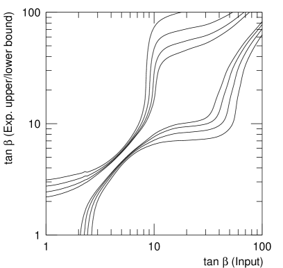
Figure 1: Accuracy of the measured $\tan\beta$ (95 % C.L.) for $\sqrt{s}=500$ GeV, $m_{H^{\pm}}=200$ GeV, $\epsilon_{b}=60$ %, and four integrated luminosities: 25, 50, 100, and 200 fb^-1 (from outside to inside).

We start with the NLC with $\sqrt{s}=500$ GeV, and the charged Higgs mass $m_{H^{\pm}}=200$ GeV. In this case, the decay of neutral Higgses into $t\bar{t}$ pair is kinematically forbidden. The $\tan\beta$ dependence of the cross sections then comes mainly from charged Higgs events. In Fig. 1, we plot the expected accuracy for $\tan\beta$ as a function of the input value (i.e., the actual value) of $\tan\beta$. Here, we use four different integrated luminosities: 25, 50, 100, and 200 fb^-1, which correspond to 0.5, 1, 2, and 4 years of running with design luminosity. The qualitative behavior of the figure can be understood in the following way. If the actual value of $\tan\beta$ is close to 1, the branching ratio of the charged Higgs decaying into $\tau\nu_{\tau}$ is too suppressed to be observed, and hence we may set an upper bound on $\tan\beta$ from the non-observation of the $H^{\pm}$ leptonic decay mode. If the underlying $\tan\beta$ is in the moderate region ($\sim$ 3 – 10), we observe both the leptonic and hadronic decays of $H^{\pm}$. In this case, we can determine $\tan\beta$ from these modes, as can be seen in Fig. 1. If the actual $\tan\beta$ is larger than $\sim 10$, pair production of heavy Higgses allows us to set a lower limit on $\tan\beta$. However, if $\tan\beta$ is large enough, the cross section for the process $e^{+}e^{-}\rightarrow tbH^{\pm}$ (channel 2) can be large enough to be observed, and both an upper and a lower limit on $\tan\beta$ can be obtained from channel 2.

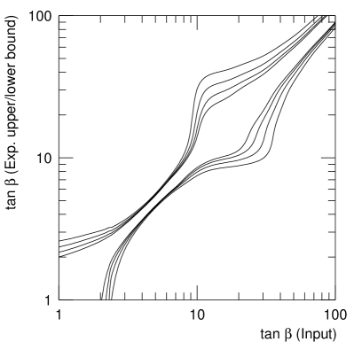
Figure 2: Accuracy of the measured $\tan\beta$ (95 % C.L.) for $\sqrt{s}=1$ TeV, $m_{H^{\pm}}=200$ GeV, $\epsilon_{b}=60$ %, and four integrated luminosities: 100, 200, 400, and 800 fb^-1 (from outside to inside).

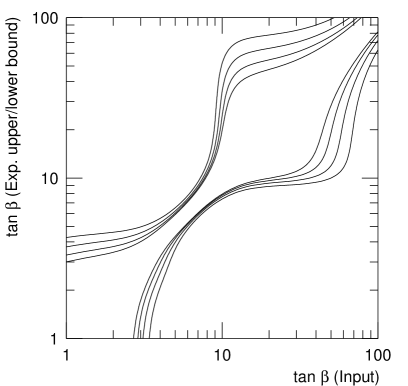
Figure 3: Same as Fig. 2, except for $m_{H^{\pm}}=300$ GeV.

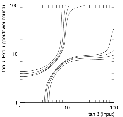
Figure 4: Same as Fig. 2, except for $m_{H^{\pm}}=400$ GeV.

If the heavy Higgses are not kinematically accessible, or even if they are, it is advantageous to increase the beam energy. Therefore, we next present results for phase II of the NLC with $\sqrt{s}=1$ TeV. In Figs. 2 – 4, we present results for $m_{H^{\pm}}=$ 200 GeV, 300 GeV, and 400 GeV, respectively. For the integrated luminosities, we use 100, 200, 400, and 800 fb^-1. In particular, for $m_{H^{\pm}}=$ 200 GeV, we can see a great improvement of the result, comparing Figs. 1 and 2. For $m_{H^{\pm}}=$ 300 GeV, we can still expect a precise determination of $\tan\beta$, especially if the underlying $\tan\beta$ is moderate or large. For $m_{H^{\pm}}=$ 400 GeV, the result is noticeably worse. There are mainly two reasons for this. First, $\sqrt{s}$ is close to the threshold energy in this case. The Higgs production cross sections then becomes small due to the phase space suppression, and the statistical errors become large. Furthermore, as the charged Higgs mass gets larger, the phase space suppression of the process $H^{\pm}\rightarrow tb$ becomes less significant, and the decay mode $H^{\pm}\rightarrow\tau\nu_{\tau}$ is relatively suppressed. As a result, the branching ratio of the charged Higgs loses its sensitivity to $\tan\beta$, contrary to the cases with $m_{H^{\pm}}=$ 200 and 300 GeV. In fact, in the case with $m_{H^{\pm}}=$ 400 GeV, $\tan\beta$ is mainly constrained by the $AH$ production process with $4b$, $2b2t$, and $4t$ final states. Note, however, that even in this case, we may distinguish low, moderate, and high $\tan\beta$, and we can still obtain accurate measurements of $\tan\beta$ if the underlying value of $\tan\beta$ is in the moderate region.

Before closing this section, we comment on the effects of the supersymmetric decay modes. Up to now, we have assumed that the Higgs bosons decay only into standard model particles. However, especially when the Higgs masses are large, Higgses may decay into superparticles, which one might think would lead to new sources of large systematic errors. Here, we would like to point out that this is not necessarily the case. Let us start with the decay mode $H\rightarrow\tilde{l}_{R}\tilde{l}_{R}^{*}$. We can predict the branching ratio for this mode, since this process is induced by $D$-term interactions. Thus, we only have to include this mode into the fit, and no new large systematic uncertainties arise. The primary effect of this decay mode is then to reduce the number of events from $AH$ production, and in fact, the numerical results are not changed much [3]. The same argument applies to the decay of $H$ into pairs of left-chirality sfermion. However, if the heavy Higgses can decay into sfermion pairs with different chirality, such as $H\rightarrow\tilde{l}_{R}\tilde{l}_{L}^{*}$, the branching ratios of the heavy Higgses depend on additional MSSM parameters, such as $\mu$ and the trilinear $A$ terms. These decay modes may then be a source of a large systematic errors. Of course, the new parameters may also be measured from different observables; for example, $\mu$ may be measured from chargino and neutralino masses, and the trilinear scalar couplings may be measured from left-right mixings. A complete analysis would therefore require a simultaneous fit to all of these parameters.

Finally, we briefly consider decays to charginos and neutralinos. These decay may be dominant in some regions of parameter space. However, if only decays to the lighter two neutralinos and the lighter chargino are available, and these are either all gaugino-like or all Higgsino-like, as is often the case, these decays are suppressed by mixing angles. If we are in the mixed region, these decay rates may be large, but in this case, all six charginos and neutralinos should be produced, and the phenomenology is quite rich and complicated.

5 DISCUSSION

The results presented in the previous section indicate that $\tan\beta$ may be well determined from the study of production and decay of the heavy Higgses at the NLC. The uncertainty in the measured $\tan\beta$ can be $O(10~{}\%)$ or less, depending on the underlying parameters. For example, for $\sqrt{s}=500$ GeV, $m_{H^{\pm}}=200$ GeV, and ${\cal L}=100$ fb^-1, the observed value $\tan\beta_{\rm obs}$ will be in the following ranges for various input values of $\tan\beta$:

$$\tan\beta~{}{\rm(input)}=2: \tan\beta_{\rm obs}<2.9,$$

$$\tan\beta~{}{\rm(input)}=3: 2.5<\tan\beta_{\rm obs}<3.6,$$

$$\tan\beta~{}{\rm(input)}=5: 4.5<\tan\beta_{\rm obs}<5.5,$$

$$\tan\beta~{}{\rm(input)}=10: 7.6<\tan\beta_{\rm obs}<30,$$

$$\tan\beta~{}{\rm(input)}=60: 40<\tan\beta_{\rm obs}<90.$$

In our study, we have not adopted any assumption which strongly depends on a specific model. Thus, if the heavy Higgses are kinematically accessible at the NLC, we can expect to obtain a constraint on $\tan\beta$ from the detailed study of heavy Higgs bosons.

Finally, we discuss implications of precise determinations of $\tan\beta$. First of all, it should be emphasized that a determination of $\tan\beta$ may help us understand physics at very high energy scales. For example, the simple SO(10) GUT predicts large values of $\tan\beta$ [17]. The unification of $m_{b}$-$m_{\tau}$ based on SU(5)-type GUTs is an another example. It prefers a value of $\tan\beta$ that is very large or close to 1 [18]. Precise determinations of $\tan\beta$ can be excellent tests of these scenarios.

The parameter $\tan\beta$ is also important for the determination of the SUSY breaking scalar masses. Neglecting mixings, the physical masses of sfermions are the sum of soft SUSY breaking masses and the $D$-term contribution which depends on $\tan\beta$. Thus, we must know $\tan\beta$ to determine soft SUSY breaking mass parameters from the physical masses of sfermions. If $\tan\beta$ is completely unknown, soft SUSY breaking masses may have large uncertainties even if we can measure the sfermion masses very accurately. Measurement of $\tan\beta$ reduce this uncertainty. The important point is that the $D$-term contribution is proportional to $\cos 2\beta$, and hence it becomes insensitive to $\tan\beta$ once $\tan\beta$ is larger than 3 – 4. Given our result, the uncertainty related to the $D$-term contribution is smaller than the error from the sfermion mass measurement, if $\tan\beta$ is larger than 3 – 4. The spectrum of the soft SUSY breaking masses may contain information about the origin of SUSY breaking [19] and the gauge and/or flavor structure at high scales [20].

Furthermore, if we combine the $\tan\beta$ determination with measurements of the Higgs masses, we may be able to gain some information about the Higgs potential. The Higgs potential is strongly constrained at the tree level, but radiative corrections are quite significant. In particular, the top squark plays an important role, and the precise determination of $\tan\beta$ as well as the Higgs masses may give us some constraint on top squark masses.

In summary, determination of the $\tan\beta$ parameter can potentially give us rich information about physics at the high scale, including the possibility of GUTs, high energy flavor structures, and the origin of SUSY breaking.

References

- [1] JLC Group, JLC-I, KEK Report 92-16.
- [2] NLC ZDR Design Group and the NLC Physics Working Group, Physics and Technology of the Next Linear Collider, SLAC-R-0485 (hep-ex/9605011); The NLC Design Group, Zeroth-Order Design Report for the Next Linear Collider, LBNL-PUB-5424.
- [3] J.L. Feng and T. Moroi, LBNL-39579 (hep-ph/9612333), to appear in Phys. Rev. D.
- [4] J.F. Gunion and J. Kelly, UCD-96-24 (hep-ph/9610495).
- [5] J.L. Feng, H. Murayama, M.E. Peskin, and X. Tata, Phys. Rev. D52 (1995) 1418.
- [6] M.M. Nojiri, K. Fujii, and T. Tsukamoto, Phys. Rev. D54 (1996) 6756.
- [7] T. Moroi, Phys. Rev. D53 (1996) 6565.
- [8] CMS Collaboration, Technical Proposal, CERN/LHCC/94-38 (1994); ATLAS Collaboration, Technical Proposal, CERN/LHCC/94-43 (1994).
- [9] J.F. Gunion, A. Stange, and S. Willenbrock, UCD-95-28 (hep-ph/9602238).
- [10] For a more complete review, see J. Gunion, H.E. Haber, G. Kane, and S. Dawson, The Higgs Hunter’s Guide (Addison-Wesley, Redwood City, California, 1990).
- [11] Y. Okada, M. Yamaguchi, and T. Yanagida, Prog. Theor. Phys. 85 (1991) 1; H.E. Haber and R. Hempfling, Phys. Rev. Lett. 66 (1991) 1815; J. Ellis, G. Ridolfi, and F. Zwirner, Phys. Lett. B257 (1991) 83; ibid, B262 (1991) 477.
- [12] J.F. Gunion, L. Poggioli, R. Van Kooten, C. Kao, and P. Rowson, UCD-97-5 (hep-ph/9703330), to appear in Proceeding of 1996 DPF/DPB Summer Study on High Energy Physics (Snowmass ’96).
- [13] C.S. Li and J.M. Yang, Phys. Lett. B315 (1993) 367; H. Konig, Mod. Phys. Lett. A10 (1995) 1113; A. Bartl, H. Eberl, K. Hidaka, T. Kon, W. Majerotto, and Y. Yamada, Phys. Lett. B378 (1996) 167; R.A. Jimenez and J. Sola, Phys. Lett. B389 (1996) 53.
- [14] A. Djouadi, H.E. Haber, and P.M. Zerwas, Phys. Lett. B375 (1996) 203.
- [15] D. Jackson, private communication.
- [16] A. Sopczak, Z. Phys. C65 (1995) 449.
- [17] B. Ananthanarayan, G. Lazarides and Q. Shafi, Phys. Rev. D44 (1991) 1613; L.J. Hall, R. Rattazzi, and U. Sarid, Phys. Rev. D50 (1994) 7048.
- [18] S. Kelly, J.L. Lopez, and D.V. Nanopoulos, Phys. Lett. B247 (1992) 387; V. Barger, M.S. Berger, and P. Ohmann, Phys. Rev. D47 (1993) 1093; P. Langacker and N. Polonsky, Phys. Rev. D49 (1994) 1454.
- [19] M.E. Peskin, Prog. Theor. Phys. Suppl. 123 (1996) 507.
- [20] T. Moroi, Phys. Lett. B321 (1994) 56; Y. Kawamura, H. Murayama, and M. Yamaguchi, Phys. Lett. B324 (1994) 52; R. Barbieri and L.J. Hall, Phys. Lett. B338 (1994) 212.