HD-THEP-97-32

hep-ph/9707489

October, 1997

Plasmon properties in classical lattice gauge theory

D. Bödeker and M. Laine

Institut für Theoretische Physik, Universität Heidelberg, Philosophenweg 16, D-69120 Heidelberg, Germany

Abstract

In order to investigate the features of the classical approximation at high temperatures for real time correlation functions, the plasmon frequencies and damping rates were recently computed numerically in the SU(2)+Higgs model and in the pure SU(2) theory. We compare the lattice results with leading order hard thermal loop resummed perturbation theory. In the broken phase of the SU(2)+Higgs model, we show that the lattice results can be reproduced and that the lattices used are too coarse to observe some important plasmon effects. In the symmetric phase, the main qualitative features of the lattice results can also be understood. In the pure SU(2) theory, on the other hand, there are discrepancies which might point to larger Landau and plasmon damping effects than indicated by perturbation theory.

PACS numbers: 11.10.Wx, 11.15.Kc, 11.30.Fs

The dynamics of non-abelian gauge fields at finite temperature has attracted some attention recently [1]–[16]. A lot of work on this subject has been done in perturbation theory. However, some physical quantities of interest are non-perturbative and the only known method of calculating them on the lattice is the classical approximation [1].

One problem of the classical approximation is related to the fact that the high momentum modes do not decouple from the dynamics of the low momentum modes. In the naive perturbative expansion, momenta of order $T$ lead to corrections in the Green’s functions which are proportional to $T^{2}$. For Green’s functions with soft external momenta $|{\bf p}|\sim g^{2}T$, where $g$ is the gauge coupling, these “corrections” can be as large as or even larger than the tree level Green’s functions. These large corrections have been named hard thermal loops (HTL) and a consistent perturbative expansion requires that they be resummed [2].

In the resummed perturbation theory the gauge field propagators reflect two distinct collective phenomena. One is the plasma oscillations which involve simultaneous oscillations of the low and the high momentum degrees of freedom in the plasma. The characteristic frequency of these oscillations is proportional to $gT$. Secondly, there is an effect called Landau damping which is related to an energy transfer from the low momentum degrees of freedom to the high momentum ones.

In the classical approximation the physics of the high momentum degrees of freedom is not correctly described. The hard thermal loops correspond to classically UV-divergent contributions [3]. How the hard thermal loops affect non-perturbative correlation functions of the low momentum fields is an open problem.

The physical picture sketched above is based on 1-loop resummed perturbation theory. It is therefore interesting to see whether it also shows up in non-perturbative lattice studies. In a recent paper [11] the correlation functions of two gauge invariant operators in the SU(2)+Higgs model (in continuum notation),

$$H(t) = \frac{1}{\sqrt{V}}\int\!\!d^{3}x\,\varphi^{\dagger}(t,{\bf x})\varphi(t,{\bf x}),$$ (1)

$$W_{i}^{a}(t) = \frac{1}{\sqrt{V}}\int\!\!d^{3}x\,i{\rm Tr\,}\left[\Phi^{\dagger}(t,{\bf x})D_{i}\Phi(t,{\bf x})\tau^{a}\right],$$ (2)

were computed with classical lattice simulations. Here $\varphi$ denotes the Higgs doublet, $\tau^{a}$ is a Pauli matrix, $\Phi$ is the matrix $\Phi=(\widetilde{\varphi}\,\varphi)$ with $\widetilde{\varphi}=i\tau^{2}\varphi^{*}$, and $V$ denotes the space volume. In the broken phase the correlator of $W_{i}^{a}(t)$ is given by the gauge field propagator. It was claimed that the plasmon frequency corresponding to this correlator is independent of the lattice spacing $a$. This contradicts the picture above since in the classical theory the plasmon frequency is proportional to $T/a$ instead of $T^{2}$. We will demonstrate here that the qualitative features of the correlators can be understood using perturbation theory and that the claim of ref. [11] concerning the broken phase $W_{i}^{a}$ plasmon frequency is not justified.

Ambjørn and Krasnitz [12] have reported a measurement of the gauge field correlator in the Coulomb gauge in the symmetric phase. We will see that many of the features observed can be qualitatively understood in perturbation theory, but quantitative discrepancies remain.

Real time correlators and the HTL effective action

The plasmon properties of the classical Hamiltonian SU(2)+Higgs gauge theory could be computed by solving the classical equations of motion perturbatively with given initial conditions, and by then averaging over the initial conditions with the Boltzmann weight [1]. However, it appears that in perturbation theory it is simpler to perform the computation in the full quantum theory and to take the classical limit $\hbar\to 0$ only in the end. We use this approach.

In the classical limit the operator ordering in a correlation function is irrelevant. Thus the quantum expression of which we are going to take the classical limit can be anything but a commutator. This still leaves several possibilities, and we choose to consider

$$C_{\cal O}(t,{\bf p})={\frac{1}{2}}\int\!d^{3}xe^{-i{\bf p}{\bf x}}\left\langle{\cal O}(t,{\bf x}){\cal O}(0,{\bf 0})+{\cal O}(0,{\bf 0}){\cal O}(t,{\bf x})\right\rangle.$$ (3)

In a perturbative computation, one first computes the corresponding two-point Green’s function ${\cal D}_{\cal O}(i\omega_{n},{\bf p})$ in Euclidean space for the Matsubara frequencies $\omega_{n}$. Then one performs an analytic continuation which depends on the real time correlator in question. The symmetric combination in eq. (3) is given by

$$C_{\cal O}(t,{\bf p})=\hbar\int_{-\infty}^{\infty}\frac{d\omega}{2\pi}e^{-i\omega t}\left[1+2n(\omega)\right]\mathop{\rm Im}{\cal D}_{\cal O}\left(i\omega_{n}\to\omega+i\epsilon,{\bf p}\right),$$ (4)

where

$$n(\omega)=\frac{1}{e^{\beta\hbar\omega}-1}\quad$$ (5)

is the Bose distribution function.

To evaluate the $\omega$-integral in eq. (4) numerically, it is convenient to rewrite it (for $t>0$) as an integral in the upper half of the complex $\omega$-plane. In this way one avoids integrating along the poles and discontinuities on the real $\omega$-axis. Denoting $\omega=\omega_{1}+i\omega_{2}$, one gets for $t>0$ in the classical limit $n(\omega)\to T/(\hbar\omega)$,

$$C_{\cal O}^{\rm classical}(t,{\bf p})=T\lim_{\hbar\to 0}{\cal D}_{\cal O}(0,{\bf p})+e^{\omega_{2}t}\int_{-\infty}^{\infty}\frac{d\omega_{1}}{2\pi i}\frac{T}{\omega_{1}+i\omega_{2}}e^{-i\omega_{1}t}\lim_{\hbar\to 0}{\cal D}_{\cal O}(\omega_{1}+i\omega_{2},{\bf p}).$$ (6)

Note that this expression is independent of the imaginary part $\omega_{2}>0$. The second term on the r.h.s. of eq. (6) vanishes for the equal time case $t=0$. A further virtue of eq. (6) is that one can take the limit ${\bf p}\to 0$ inside the integrand since $\omega_{2}>0$ guarantees that there are no singularities on the integration contour. In the remainder of this letter we will discuss only classical correlation functions and we will therefore omit the superscript ’classical’ from the l.h.s. of eq. (6).

We thus have to evaluate ${\cal D}_{\cal O}(\omega,{\bf p})$. As discussed above, a consistent perturbative expansion requires the resummation of the hard thermal loops [2]. In other words, the high momentum modes $p\mathop{\raise 1.29167pt\hbox{$>$\kern-7.5pt\raise-4.73611pt\hbox{$\sim$}}}T$ (or $p\mathop{\raise 1.29167pt\hbox{$>$\kern-7.5pt\raise-4.73611pt\hbox{$\sim$}}}a^{-1}$ in the classical theory) are integrated out, giving an effective theory for the low momentum modes $p\mathop{\raise 1.29167pt\hbox{$<$\kern-7.5pt\raise-4.73611pt\hbox{$\sim$}}}gT$. This amounts to including the hard thermal loops in the tree level action. Denoting $P=(\omega_{n},{\bf p})$, the quadratic part of the Euclidean HTL effective theory in momentum space is

$${\cal L}_{\rm HTL}^{(2)}={\frac{1}{2}}A_{\mu}^{a}A_{\nu}^{a}\left[P^{2}\delta^{\mu\nu}-P^{\mu}P^{\nu}+\Pi_{\rm HTL}^{\mu\nu}(P)\right]+\varphi^{\dagger}\varphi\left[P^{2}-{\frac{1}{2}}m_{H}^{2}+\Sigma_{\rm HTL}\right],$$ (7)

where $m_{H}$ is the Higgs mass. Eq. (7) gives directly the gauge and scalar field free propagators ${\cal D}_{\mu\nu}^{ab}(\omega,{\bf p})$, ${\cal D}(\omega,{\bf p})$, to be used in the computation of ${\cal D}_{\cal O}(\omega,{\bf p})$. Note that $\Sigma_{\rm HTL}$ is momentum independent.

Of the HTL self-energies, we will need especially the components $\Pi_{\rm HTL}^{ij}(P)$, $\Sigma_{\rm HTL}$. The expressions are [2, 3, 10], after the replacement $\omega_{n}\to-i\omega$,

$$\Pi_{\rm HTL}^{ij}(P) = -g^{2}(2N+N_{\rm s})\hbar\int\!\!\frac{d^{3}q}{(2\pi)^{3}}\,\frac{dn(\omega_{q})}{d\omega_{q}}\frac{v^{i}v^{j}\omega}{\omega-p^{i}v^{i}},$$ (8)

$$\Sigma_{\rm HTL} = \left(6\lambda+\frac{9}{4}g^{2}\right)\hbar\int\!\!\frac{d^{3}q}{(2\pi)^{3}}\,\frac{n(\omega_{q})}{\omega_{q}},$$ (9)

where, for the SU(2)+Higgs model, $N=2$, $N_{\rm s}=1$. Furthermore,

$$v^{i}=\frac{\partial\omega_{q}}{\partial q_{i}}$$ (10)

where $\omega_{q}$ is the tree level dispersion relation; for a space-time with discretized spatial dimensions (a cubic lattice),

$$\omega_{q}=\frac{2}{a}\sqrt{{\textstyle\sum_{i}}\sin^{2}\!\left(aq_{i}/2\right)},\quad v^{i}=\frac{\sin(aq^{i})}{a\omega_{q}}.$$ (11)

Eqs. (8), (9) hold actually for a generic dispersion relation [10]. In ref. [3], scalar electrodynamics was considered for which case $g^{2}(2N+N_{\rm s})$ has to be replaced with $2e^{2}$ in eq. (8).

Note that in the theory of eq. (7), the gauge field $A_{0}$ is included. In the classical lattice simulations [11, 12], in contrast, one puts $A_{0}=0$ and imposes the Gauss constraint explicitly.

The hard thermal loop self-energy simplifies in the limit ${\bf p}=0$, which is relevant for the operators in eqs. (1), (2). In that limit, the gauge field self-energy is

$$\Pi_{\rm HTL}^{00}=0,\quad\Pi_{\rm HTL}^{0i}=0,\quad\Pi_{\rm HTL}^{ij}=\delta^{ij}\omega_{W}^{2},$$ (12)

where $\omega_{W}$ is the plasmon frequency,

$$\omega_{W}^{2}=-{\frac{1}{3}}g^{2}(2N+N_{\rm s})\hbar\int\!\frac{d^{3}q}{(2\pi)^{3}}\frac{dn(\omega_{q})}{d\omega_{q}}|{\bf v}|^{2}.$$ (13)

Let us also introduce the “scalar plasmon frequency”

$$\omega_{H}^{2}=-{\frac{1}{2}}m_{H}^{2}+\Sigma_{\rm HTL}.$$ (14)

In the continuum limit of the full quantum theory, for which $|{\bf v}|^{2}=1$, one has

$$\omega_{W}^{2} = g^{2}(2N+N_{\rm s})\frac{T^{2}}{18}\frac{1}{\hbar},$$ (15)

$$\omega_{H}^{2} = -{\frac{1}{2}}m_{H}^{2}+\left(6\lambda+{\frac{9}{4}}g^{2}\right)\frac{T^{2}}{12}\frac{1}{\hbar},$$ (16)

whereas in the classical limit $n(\omega)\to T/(\hbar\omega)$ on a cubic lattice, one gets

$$\omega_{W}^{2} = g^{2}(2N+N_{\rm s})\left({\frac{3}{2}}\frac{\Sigma}{\pi}-1\right)\frac{T}{12a},$$ (17)

$$\omega_{H}^{2} = -{\frac{1}{2}}m_{H}^{2}+\left(6\lambda+{\frac{9}{4}}g^{2}\right)\frac{\Sigma}{4\pi}\frac{T}{a}.$$ (18)

Here

$$\Sigma=\frac{1}{\pi^{2}}\int_{-\pi/2}^{\pi/2}\!\!d^{3}x\frac{1}{\sum_{i}{\sin}^{2}x_{i}}=3.175911535625$$ (19)

is a constant which can be expressed in terms of the complete elliptic integral of the first kind [17].

The basic problem of the classical real time simulations can now be expressed as follows. For the scalar field, one has a mass parameter in the classical SU(2)+Higgs theory which does not break gauge invariance. It can be tuned such that the high momentum modes produce the correct quantum expression in eq. (16), and that the lattice spacing dependence in eq. (18) is canceled. For the gauge fields, in contrast, the local classical SU(2)+Higgs theory does not allow a mass term and hence the divergent classical expression in eq. (17) cannot be arranged to coincide with the quantum expression in eq. (15). This divergence should also show up in the classical simulations. This problem is specific for time dependent correlation functions: in the static case only the $\omega_{n}=0$ sector requires a resummation and $\Pi_{\rm HTL}^{ij}(0,{\bf p})=0$.

Finally, let us fix some notation. The continuum field $\varphi$ in eqs. (1), (2) is related to the dimensionless lattice field $\bar{\varphi}$ in [11] by

$$\bar{\varphi}^{\dagger}\bar{\varphi}=\frac{a}{T\beta_{G}}\varphi^{\dagger}\varphi,\quad\beta_{G}=\frac{4}{ag^{2}T}.$$ (20)

The operators measured on the lattice are then

$$\bar{H} = \frac{1}{\sqrt{N^{3}}}\sum_{\bf x}\bar{\varphi}^{\dagger}({\bf x})\bar{\varphi}({\bf x}),$$ (21)

$$\bar{W}^{a}_{i} = \frac{1}{\sqrt{N^{3}}}\sum_{\bf x}i{\rm Tr\,}\left[\bar{\Phi}^{\dagger}({\bf x})U_{i}({\bf x})\bar{\Phi}({\bf x}+{\bf e}_{i}a)\tau^{a}\right],$$ (22)

where $U_{i}({\bf x})$ is the link operator. The correlators measured with these operators are denoted by $C_{\bar{H}}(t)$, ${\frac{1}{3}}\delta^{ab}\delta_{ij}C_{\bar{W}}(t)$, and they are related in the continuum limit $a\to 0$ to the correlators $C_{H}(t),C^{ab}_{W,ij}(t)$ of the continuum operators in eqs. (1), (2) through $C_{H}(t)=a\beta_{G}^{2}T^{2}C_{\bar{H}}(t)$, $C^{ab}_{W,ij}(t)={\frac{1}{3}}\delta^{ab}\delta_{ij}a^{-1}\beta_{G}^{2}T^{2}C_{\bar{W}}(t)$. The factor $3$ in the definition of $C_{\bar{W}}(t)$ corresponds to a sum over the different isospin components.

The broken phase

Let us first consider the broken phase. The real time correlators of the operators $\bar{H}(t)$, $\bar{W}^{a}_{i}(t)$ have been determined in the classical approximation in the broken phase of the SU(2)+Higgs model by Tang and Smit [11].

We parameterize the scalar field in the broken phase as

$$\Phi=\frac{1}{\sqrt{2}}\left[v(T)+\phi_{0}+i\tau^{a}\phi_{a}\right].$$ (23)

Then, in continuum notation, the lowest order terms in the gauge invariant operators of eqs. (1), (2) become

$$H(t) = {\rm const.}+\frac{1}{\sqrt{V}}\int\!\!d^{3}x\,v(T)\phi_{0}(t,{\bf x}),$$ (24)

$$W^{a}_{i}(t) = \frac{1}{\sqrt{V}}\int\!\!d^{3}x\,v(T)\Bigl{[}m_{W}(T)A^{a}_{i}(t,{\bf x})-\partial_{i}\phi_{a}(t,{\bf x})\Bigr{]},$$ (25)

where $m_{W}(T)=gv(T)/2$. Due to the integration $\int\!d^{3}x$, these operators correspond to zero spatial momentum, ${\bf p}=0$, so that the second term in eq. (25) does not contribute. It follows that the leading terms in the correlation functions $C_{H}(t)$ and $C^{ab}_{W,ij}(t)$ are given by the propagators of the elementary fields $\phi_{0}$ and $A^{a}_{i}$.

To compute the required propagators, one can set ${\bf p}=0$ in the time dependent part of eq. (6), so that eqs. (13), (14) can be used. At zero spatial momentum the full Euclidean (Matsubara) propagators for the fields $A^{a}_{i}$, $\phi_{0}$ are of the form

$${\cal D}_{ij}^{ab}(i\omega_{n},{\bf 0})=\frac{\delta^{ab}\delta_{ij}}{\omega_{n}^{2}+(\omega_{W}^{\rm b})^{2}+\mbox{${}^{\ast}\Pi(i\omega_{n})$}},\quad{\cal D}(i\omega_{n},{\bf 0})=\frac{1}{\omega_{n}^{2}+(\omega_{H}^{\rm b})^{2}+\mbox{${}^{\ast}\Sigma(i\omega_{n})$}},$$ (26)

where ${}^{\ast}\Pi$, ${}^{\ast}\Sigma$ denote the parts of the self-energies which are generated radiatively within the HTL effective theory. The tree-level terms are

$$(\omega_{W}^{\rm b})^{2} = m_{W}^{2}(T)+0.05379\beta_{G}(g^{2}T)^{2},$$ (27)

$$(\omega_{H}^{\rm b})^{2} = m^{2}_{H}(T),$$ (28)

where $m_{W}(T)$, $m_{H}(T)$ are the mass parameters generated by the Higgs mechanism in the static theory: $m_{W}(T)=gv(T)/2$, $m_{H}^{2}(T)=\omega_{H}^{2}+3\lambda v^{2}(T)$. Here the scalar mass parameter was tuned to its correct value by using the counterterm of the static classical theory and the fact that $\Sigma_{\rm HTL}$ is momentum independent. For $(\omega_{W}^{\rm b})^{2}$, in contrast, the $\beta_{G}$-dependent part comes from eq. (17) and cannot be removed. Parametrically, $(\omega^{\rm b})^{2}\sim g^{2}T^{2}$ and ${}^{\ast}\Pi(\omega_{W}^{\rm b})$, ${}^{\ast}\Sigma(\omega_{H}^{\rm b})\sim g^{3}T^{2}$, so that the dominant contributions to the $H$ and $W^{a}_{i}$ plasmon frequencies (appearing as $C(t,{\bf p})\sim C_{0}\exp({-\Gamma t})\cos(\omega_{\rm pl}t+\delta)$ in the correlator) are just $\omega_{H}^{\rm b}$ and $\omega^{\rm b}_{W}$ according to eq. (6). The damping rates $\Gamma$ are related to ${}^{\ast}\Pi(\omega_{W}^{\rm b})$ and ${}^{\ast}\Sigma(\omega_{H}^{\rm b})$.

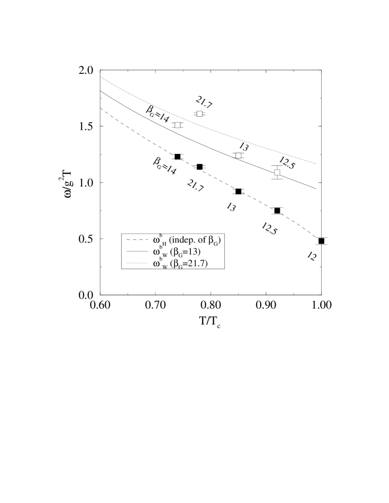
Figure 1: A comparison of the leading order perturbative plasmon frequencies with those determined on the lattice in [11]. The continuous curves are the perturbative values from eqs. (27), (28), and the squares are the data points from Table 5 in [11]. Open symbols correspond to $\omega_{W}^{\rm b}$ and filled to $\omega_{H}^{\rm b}$. The corresponding $\beta_{G}$ values are given next to the symbols.

In Fig. 1 we compare the leading order plasmon frequencies in eqs. (27), (28) with the lattice results of ref. [11]. The value of $v(T)$ has been determined from the 1-loop effective potential. The zero-temperature parameters used in [11] correspond to $m_{H}$ = 80 GeV. It is seen that the lattice results are remarkably close to the leading order perturbative results. In particular, we conclude that the gauge field plasmon frequency $\omega_{W}^{\rm b}$ diverges in the continuum limit according to eq. (27), while the scalar plasmon frequency $\omega_{H}^{\rm b}$ remains finite and equals the static screening mass at leading order. One sees that the lattice is so coarse that it is difficult to notice the divergence of $\omega_{W}^{\rm b}$ since this is shadowed by the finite $m_{W}(T)$. Thus one is in a sense not close enough to the continuum limit. It should also be noted that the amplitude of $C^{ab}_{W,ij}(t)$ dies out as $1/(\omega_{W}^{\rm b})^{2}$ in the continuum limit.

The damping rates of the gauge and scalar fields are parametrically of order $g^{2}T$ and therefore, in contrast to the plasmon frequencies, they are classical. This has been demonstrated explicitly in a scalar field theory [13, 14]. A full computation of the damping rates in the broken phase of the SU(2)+Higgs theory is missing at the moment. However, the order of magnitude can apparently be understood [11] using the known symmetric phase gauge and Higgs elementary field damping rates [18, 19].

The symmetric phase

Let us now turn to the symmetric phase. The correlators of the composite operators in eqs. (1), (2) have been determined in the symmetric phase of the SU(2)+Higgs model by Tang and Smit [11]. In addition, the gauge field correlator of the pure SU(2) model has been measured in the Coulomb gauge by Ambjørn and Krasnitz [12].

Consider first the composite operator correlators measured in [11]. In the symmetric phase, the composite operator character of $H(t)$ and $W^{a}_{i}(t)$ manifests itself more clearly than in the broken phase. For instance, the leading term in $\bar{W}^{a}_{i}$ is

$$\bar{W}^{a}_{i}=\frac{1}{\sqrt{N^{3}}}\sum_{\bf x}\left[\bar{\phi}_{0}({\bf x}+{\bf e}_{i}a)\bar{\phi}_{a}({\bf x})-\bar{\phi}_{0}({\bf x})\bar{\phi}_{a}({\bf x}+{\bf e}_{i}a)-\epsilon^{abc}\bar{\phi}_{b}({\bf x})\bar{\phi}_{c}({\bf x}+{\bf e}_{i}a)\right],$$ (29)

which does not contain the gauge field $A^{a}_{i}$ at all.

Figure 2: The lowest order diagram contributing to $C_{H}(t)$ and $C^{ab}_{W,ij}(t)$ in the symmetric phase. The solid lines denote scalar propagators.

Due to the fact that no gauge fields are involved, the leading terms in $C_{H}(t)$ and $C^{ab}_{W,ij}(t)$ can be easily computed: both are given by diagrams of the type depicted in Fig. 2. To evaluate them one has to start with a Matsubara external momentum $p_{0}=i\omega_{n}$. Then the sum over the loop frequencies is written in terms of an integral in the complex $k_{0}$ plane (see, e.g., [20]). Only then can one continue to arbitrary complex values of $p_{0}$. For the operator ${\cal O}(t,{\bf x})=\varphi^{\dagger}\varphi(t,{\bf x})$, the diagram in Fig. 2 finally gives

$${\rm Im}{\cal D}_{\varphi^{\dagger}\varphi}(p_{0}+i\epsilon,{\bf p})=$$

$$\quad\quad 4\int\!\frac{d^{4}k}{(2\pi)^{4}}\left[n(k_{0})-n(k_{0}+p_{0})\right]{\rm Im}{\cal D}(k_{0}+i\epsilon,{\bf k})\,{\rm Im}{\cal D}(k_{0}+p_{0}+i\epsilon,{\bf k}+{\bf p}).\hskip 28.45274pt$$ (30)

This expression is equivalent to a corresponding one derived in ref. [21]. The correlator $C_{H}(t)={\frac{1}{2}}\langle H(t)H(0)+H(0)H(t)\rangle$ for the operator $H(t)$ of eq. (1) is given by $C_{H}(t)=C_{\varphi^{\dagger}\varphi}(t,{\bf p}=0)$, where $C_{\varphi^{\dagger}\varphi}(t,{\bf p})$ is obtained from eq. (4).

To get the leading contribution in $C_{H}(t)$, one uses the free propagators for which

$${\rm Im}{\cal D}_{\rm free}(k_{0}+i\epsilon,{\bf k})=\frac{\pi}{2\sqrt{{\bf k}^{2}+\omega_{H}^{2}}}\left[\delta\left(k_{0}-\sqrt{{\bf k}^{2}+\omega_{H}^{2}}\right)-\delta\left(k_{0}+\sqrt{{\bf k}^{2}+\omega_{H}^{2}}\right)\right].$$ (31)

Then the integrals over $k_{0}$ and $p_{0}$ can be performed in eqs. (30), (4). In the limit ${\bf p}\to 0$, one obtains

$$C_{H}(t)=T^{2}\int\frac{d^{3}k}{(2\pi)^{3}}\frac{1}{({\bf k}^{2}+\omega_{H}^{2})^{2}}\left[1+\cos\left(2\sqrt{{\bf k}^{2}+\omega_{H}^{2}}\,t\right)\right].$$ (32)

On the lattice (in the continuum limit) this corresponds to

$$C_{\bar{H}}(t)=\frac{1}{4\pi^{2}\beta_{G}^{2}}\int_{0}^{\infty}dx\frac{x^{2}}{(x^{2}+z^{2})^{2}}\left[1+\cos(4\bar{t}\sqrt{x^{2}+z^{2}})\right],$$ (33)

where $z=a\omega_{H}/2$ and $\bar{t}=t/a$.

The vector correlator $C^{ab}_{W,ij}(t)$ has an additional factor of $k_{i}k_{j}$ in the integrand compared with eq. (32). Therefore the continuum limit of $C^{ab}_{W,ij}(t=0)$ does not exist. On the lattice one obtains

$$C_{\bar{W}}(t)=\frac{2}{\pi^{3}\beta_{G}^{2}}\int_{0}^{\pi/2}\!d^{3}x\frac{\sum_{i}\sin^{2}2x_{i}}{[\sum_{i}\sin^{2}x_{i}+z^{2}]^{2}}\left[1+\cos\left(4\bar{t}\sqrt{{\textstyle\sum_{i}}\sin^{2}x_{i}+z^{2}}\right)\right].$$ (34)

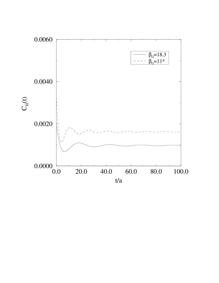
Figure 3: The leading order perturbative correlator $C_{\bar{H}}(t)$ in lattice units in the symmetric phase at $T/T_{c}=1.52$. To be compared with Fig. 8 in [11]. The oscillation frequency is $2\omega_{H}$ (this agrees at leading order with the static screening mass).

Figure 4: The leading order perturbative correlator $C_{\bar{W}}(t)$ in lattice units in the symmetric phase at $T/T_{c}=1.52$. To be compared with Fig. 10 in [11]. The oscillation period here is proportional to the lattice spacing $a$.

The correlation function $C_{\bar{H}}(t)$ is shown in Fig. 3 and $C_{\bar{W}}(t)$ in Fig. 4. These should be compared with Figs. 8, 10 in [11], respectively. It is seen that the qualitative features can be understood quite well with the leading order results. Note, in particular, that the scalar correlation function $C_{\bar{H}}(t)$ in Fig. (3) is oscillating with an amplitude which decreases with time. It should be emphasized that this decrease is not related to damping (remember that Fig. 3 shows the tree level results without any interactions and damping occurs only through interactions). The decrease is rather due to the fact that there is a continuous spectrum of frequencies $\omega>2\omega_{H}$ causing a destructive interference in the phase space integral, eq. (33). This shows that it is difficult to determine a damping rate from the gauge invariant operator $C_{\bar{H}}(t)$.

Let us then try to estimate how higher order corrections could modify the qualitative behavior of $C_{H}(t)$. Consider the effect of self-energy insertions in the scalar propagators ${\cal D}(k_{0},{\bf k})$. The self-energy has an imaginary part. Therefore the scalar propagator does not have poles at $k_{0}=\pm\sqrt{{\bf k}^{2}+\omega_{H}^{2}}$ (the lowest order result for $C_{H}(t)$ is due to these poles). Since the imaginary part of the self-energy is small compared with $\sqrt{{\bf k}^{2}+\omega_{H}^{2}}$, $C_{H}(t)$ will nevertheless still be dominated by the region $k_{0}\approx\pm\sqrt{{\bf k}^{2}+\omega_{H}^{2}}$. One can therefore approximate the scalar propagator as

$${\cal D}(k_{0}+i\epsilon,{\bf k})\approx\frac{1}{-(k_{0}+i\Gamma_{k})^{2}+{\bf k}^{2}+\omega_{H}^{2}},$$ (35)

where the width $\Gamma_{k}$ is given by (see, e.g., [21]) $\Gamma_{k}\equiv-{\rm Im}\Sigma(\sqrt{{\bf k}^{2}+\omega_{H}^{2}},{\bf k})/(2\sqrt{{\bf k}^{2}+\omega_{H}^{2}})$. Inserting this into eq. (30) and using eq. (4), we find

$$C_{H}(t)=T^{2}\int\frac{d^{3}k}{(2\pi)^{3}}\frac{e^{-2\Gamma_{k}t}}{[{\bf k}^{2}+\omega_{H}^{2}][{\bf k}^{2}+\omega_{H}^{2}+\Gamma_{k}^{2}]}\left[1+\cos\left(2\sqrt{{\bf k}^{2}+\omega_{H}^{2}}\,t-2\alpha_{k}\right)\right],$$ (36)

where $\alpha_{k}=\arctan\left({\Gamma_{k}}/{\sqrt{{\bf k}^{2}+\omega_{H}^{2}}}\right)$. Thus the effect of damping should show up in Fig. 3 such that the constant part (corresponding to the first term in the square brackets in eq. (36)) decays away at large times. This is indeed the qualitative behavior observed in [11].

Finally, we consider the transverse gauge field correlator $C_{A_{\scriptstyle\rm t}}(t,{\bf p})$ measured in [12]. Gauge fields can only be defined in a particular gauge, which in [12] was chosen to be the Coulomb gauge. We let the external momentum point into the $x_{3}$-direction, ${\bf p}={\bf e}_{3}(2\pi k/L)$, where $L$ is the spatial extent of the lattice and $k$ is an integer. Then $C_{A_{\scriptstyle\rm t}}(t,{\bf p})$ is given, e.g., by the correlator of $A_{1}^{a}$,

$$C_{A_{\scriptstyle\rm t}}(t,{\bf p})=\frac{1}{2}\int d^{3}xe^{-i{\bf p}{\bf x}}\langle A_{1}^{a}(t,{\bf x})A_{1}^{a}(0,{\bf 0})+A_{1}^{a}(0,{\bf 0})A_{1}^{a}(t,{\bf x})\rangle.$$ (37)

Let us first recall some features of $C_{A_{\scriptstyle\rm t}}(t,{\bf p})$ and of the corresponding analytic Green’s function ${\cal D}_{A_{\scriptstyle\rm t}}(\omega,{\bf p})$ for $|{\bf p}|\sim g^{2}T$ in the quantum theory. After the HTL resummation, ${\cal D}_{A_{\scriptstyle\rm t}}(\omega,{\bf p})$ has poles at $\omega\approx\pm\omega_{W}$, where $\omega_{W}$ is given by eq. (15). These poles lead to an oscillation of $C_{A_{\scriptstyle\rm t}}(t,{\bf p})$ on the time scale $\sqrt{\hbar}/(gT)$. In addition, ${\cal D}_{A_{\scriptstyle\rm t}}(\omega,{\bf p})$ has a discontinuity on the real $\omega$-axis for $\omega<|{\bf p}|$. This discontinuity is related to Landau damping and it gives a contribution $f_{\rm Landau}(t,{\bf p})$ to $C_{A_{\scriptstyle\rm t}}(t,{\bf p})$. The function $f_{\rm Landau}(t,{\bf p})$ does not involve any oscillations and just constitutes a decaying background for the superimposed plasmon oscillations. The time scale on which $f_{\rm Landau}(t,{\bf p})$ varies is $\mathop{\raise 1.29167pt\hbox{$>$\kern-7.5pt\raise-4.73611pt\hbox{$\sim$}}}1/(g^{2}T)$.

Higher order corrections to ${\cal D}_{A_{\scriptstyle\rm t}}(\omega,{\bf p})$, which are not included in HTL effective action but are generated radiatively within that theory, lead to a damping of the plasmon oscillations. The plasmon damping rate $\Gamma$ is of order $g^{2}T$ and has been computed for ${\bf p}=0$ in ref. [18].

These two different damping effects manifest themselves in the correlator $C_{A_{\scriptstyle\rm t}}(t,{\bf p})$ in quite different ways, so that its functional form is expected to be

$$C_{A_{\scriptstyle\rm t}}(t,{\bf p})\sim A\exp({-\Gamma t})\cos(\omega_{W}t+\delta)+f_{\rm Landau}(t,{\bf p}).$$ (38)

The time dependence of $f_{\rm Landau}(t,{\bf p})$ becomes non-perturbative for $t\mathop{\raise 1.29167pt\hbox{$>$\kern-7.5pt\raise-4.73611pt\hbox{$\sim$}}}1/(\hbar g^{4}T)$ [7], where $f_{\rm Landau}(t,{\bf p})$ is expected to vanish. This means that $C_{A_{\scriptstyle\rm t}}(t,{\bf p})$ can be computed perturbatively up to a non-perturbative constant $C_{A_{\scriptstyle\rm t}}(0,{\bf p})$ as long as $t\ll 1/(\hbar g^{4}T)$.

In the classical lattice gauge theory one expects a similar qualitative behavior. In the order of magnitude estimates for the quantum theory one has to replace $\hbar\to Ta$. The analytic structure of ${\cal D}_{A_{\scriptstyle\rm t}}(\omega,{\bf p})$ is more complicated than in the quantum case. The HTL resummed ${\cal D}_{A_{\scriptstyle\rm t}}(\omega,{\bf p})$ depends not only on the magnitude but also on the direction of ${\bf p}$ [3]. In particular, there are directions of ${\bf p}$ for which there is a discontinuity for arbitrarily large values of $\omega$ [10]. Nevertheless, the qualitative behavior of $C_{A_{\scriptstyle\rm t}}(t,{\bf p})$ should be given by eq. (38).

Unfortunately, the numerical results for $C_{A_{\scriptstyle\rm t}}(t,{\bf p})$ in [12] have been normalized to $C_{A_{\scriptstyle\rm t}}(0,{\bf p})$ which cannot be computed in perturbation theory. Comparing our perturbative estimates with the non-perturbative results therefore requires some model assumptions about $C_{A_{\scriptstyle\rm t}}(0,{\bf p})$.

In order to account for the plasmon damping effects, we include the leading order damping rate $\Gamma$ in the HTL resummed propagator ${\cal D}^{ab}_{ij}(\omega,{\bf p})$. Since the momentum dependence of $\Gamma$ is not known we use its value for ${\bf p}=0$ which is $\Gamma=0.176g^{2}T$ [18]. We can then write for the transverse components in eq. (37), analogously to eq. (35),

$${\cal D}^{ab}_{11}(\omega+i\epsilon,{\bf p})=\frac{\delta^{ab}}{-(\omega+i\Gamma)^{2}+{\bf p}^{2}+\Pi_{\rm HTL}^{11}(\omega,{\bf p})}.$$ (39)

Consider first the zero external momentum case, ${\bf p}={\bf 0}$. Eq. (39) only makes sense when $\Gamma^{2}\ll{\bf p}^{2}+\mathop{\rm Re}\Pi^{11}_{\rm HTL}(\omega,{\bf p})$. In the latter term in eq. (6) there should be no problem, since for ${\bf p}=0$, $\Pi^{11}_{\rm HTL}(\omega,{\bf p})\to\omega_{W}^{2}$, but for the first term (i.e., for the static limit $t=0$) the inequality is not satisfied (remember that $\Pi_{\rm HTL}^{11}(0,{\bf p})=0$). One might try to regulate the real part of the gauge fixed self-energy phenomenologically with a “magnetic mass”; letting $M=\sqrt{m_{\rm magn}^{2}+\Gamma^{2}+\omega_{W}^{2}}$, $\widetilde{M}=\sqrt{m_{\rm magn}^{2}+\omega_{W}^{2}}$, it follows from eq. (6) that this would give

$$C_{A_{\scriptstyle\rm t}}(0) = \frac{T}{m_{\rm magn}^{2}+\Gamma^{2}},$$ (40)

$$C_{A_{\scriptstyle\rm t}}(t)-C_{A_{\scriptstyle\rm t}}(0) = -\frac{T}{M^{2}}+\frac{T}{M\widetilde{M}}e^{-\Gamma t}\cos\!\left(\widetilde{M}t-\arctan\frac{\Gamma}{\widetilde{M}}\right).$$ (41)

Parameterized this way, one can indeed find quite reasonable agreement with Fig. 6 in [12], but only if $\Gamma$ is chosen to have a large value, $\Gamma\sim(0.8\ldots 1.0)g^{2}T$. Otherwise one is getting too many oscillations in $C_{A_{\scriptstyle\rm t}}(t)$, not observed in [12]. For these large values of $\Gamma$, the magnetic mass parameter is in fact favored to be small or zero. However, these fits are quite phenomenological, and thus we will not consider them any more.

For ${\bf p}\neq 0$, the $t=0$ –part of the leading order correlator is still parametrically non-perturbative, but at least it is formally finite for $\Gamma\to 0$ so that the perturbative approximation might be numerically reasonable. To get a feeling about the momentum scales in question, note that for the value $\beta_{G}=14$ considered in [12], $|{\bf p}|=0.69g^{2}T\times k$ and $\omega_{W}=0.87g^{2}T$ (the latter can be obtained from eq. (27) with $m_{W}(T)=0$). We have evaluated numerically both the HTL self-energy in eq. (8) and the remaining $\omega_{1}$-integral in eq. (6), for $k=1,\ldots,4$. The resulting correlators are shown in Fig. 5. This should be compared with Fig. 6 in [12].

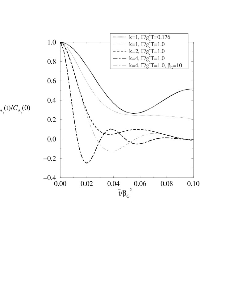
Figure 5: The gauge field correlator in the pure SU(2) theory. To be compared with Fig. 6 in [12]. Here $t$ is expressed in lattice units: $\bar{t}\equiv t/a$. Unless otherwise stated, $\beta_{G}=14$.

The main effects to be seen in Fig. 5 are the following. For $k=1$ one can see an oscillation in Fig. 5, in contrast to Fig. 6 in [12]. Thus one could say that the non-perturbative plasmon damping rate is larger than the perturbative estimate $\Gamma=0.176g^{2}T$. Indeed, one has to go to a much larger value, $\Gamma\sim 1.0g^{2}T$ ($>|{\bf p}|,\omega_{W}$), to get enough plasmon damping. Another observation to be made at $k=1$ is that in [12] the correlator is already very close to zero at $\bar{t}/\beta_{G}^{2}=0.10$. This is not quite so in Fig. 5, but one has to wait much longer for the correlator to vanish. Thus the non-perturbative Landau damping effects seem also to be larger than the leading order perturbative HTL result. At $k=2$ there is no large difference in Landau damping any more, but the plasmon damping appears to be somewhat too weak even with $\Gamma\sim 1.0g^{2}T$. Finally, at $k=4$ one gets reasonable agreement between the perturbative and lattice results, provided that $\Gamma\sim 1.0g^{2}T$. One can also see that the $\beta_{G}$-dependence is reproduced; the plasmon frequency thus diverges according to eq. (17).

We have also tried the expression $-\omega^{2}-2i\omega\Gamma$ in the denominator of eq. (39), so that the real part is not modified by $\Gamma^{2}$. The qualitative conclusions and the preferred value $\Gamma\sim 1.0g^{2}T$ remain the same. Based on those curves, one would nevertheless say that even at $k=2$ there is too little Landau damping in the perturbative estimates, but at $k=4$ one again gets good agreement.

Summary and Conclusions

We have computed several quantities related to real time correlation functions in the classical SU(2) and SU(2)+Higgs models on the lattice, using hard thermal loop resummed perturbation theory.

Our results for the gauge field and scalar plasmon frequencies in the broken phase are in remarkable agreement with the numerical lattice simulations in ref. [11]. We have reiterated that the classical gauge field plasmon frequency is divergent in the continuum limit and we have demonstrated that this is consistent with the results of ref. [11], where the plasmon frequency was claimed to be lattice spacing independent.

For the symmetric phase we have computed gauge invariant scalar and vector correlators as functions of time at the lowest order in perturbation theory. Furthermore, we have estimated the effect of higher order corrections. Our results are in good agreement with ref. [11]. We have shown that it is difficult to extract damping rates from the measurement of these correlators.

Finally, we have studied the correlator of the transverse gauge field in pure SU(2) gauge theory. While the qualitative features of the numerical simulations in ref. [12] are consistent with our perturbative estimates, there appear to be significant quantitative discrepancies. The damping of the plasmon oscillations observed in [12] appears to be much stronger than one would expect from the perturbative result for the damping rate [18]. This is puzzling because the damping rate is of the order $g^{2}T$ and should therefore have a classical continuum limit. However, one should keep in mind that the perturbative estimates are reliable only if the plasmon frequency is much larger than the damping rate which is not the case for the lattice spacing used in ref. [12].

Acknowledgments. We are grateful to E. Berger, P. Overmann, O. Philipsen, M.G. Schmidt and I.O. Stamatescu for useful discussions.

Note added

After this paper was submitted, we were informed by J.Smit that in the revised version of Ref. [11], Tang and Smit have weakened their conclusions concerning the lattice spacing independence of the $W$ plasmon frequency in the broken phase, so that their statements are now in better accordance with ours. We thank J.Smit for communication on this issue.

In view of the interpretation in [22], let us stress that the discussion around eq. (35) is not meant to be a consistent quantitative estimate of the higher order corrections. We just want to see in which qualitative way the higher order corrections might manifest themselves.

References

- [1] D.Yu. Grigoriev and V.A. Rubakov, Nucl. Phys. B 299 (1988) 67.
- [2] E. Braaten and R. Pisarski, Nucl. Phys. B 337 (1990) 569; Phys. Rev. D 45 (1992) 1827; J. Frenkel and J.C. Taylor, Nucl. Phys. B 334 (1990) 199; J.C. Taylor and S.M.H. Wong, Nucl. Phys. B 346 (1990) 115.
- [3] D. Bödeker, L. McLerran and A. Smilga, Phys. Rev. D 52 (1995) 4675.
- [4] J. Ambjørn and A. Krasnitz, Phys. Lett. B 362 (1995) 97.
- [5] G.D. Moore, Nucl. Phys. B 480 (1996) 657; Nucl. Phys. B 480 (1996) 689; PUPT-1698 [hep-ph/9705248]; G.D. Moore and N. Turok, Phys. Rev. D 55 (1997) 6538; PUPT-1681 [hep-ph/9703266].
- [6] W-H. Tang and J. Smit, Nucl. Phys. B 482 (1996) 265.
- [7] P. Arnold, D. Son and L.G. Yaffe, Phys. Rev. D 55 (1997) 6264.
- [8] P. Huet and D.T. Son, Phys. Lett. B 393 (1997) 94.
- [9] C.R. Hu and B. Müller, DUKE-TH-96-133 [hep-ph/9611292].
- [10] P. Arnold, Phys. Rev. D 55 (1997) 7781.
- [11] W-H. Tang and J. Smit, ITFA-97-02 [hep-lat/9702017].
- [12] J. Ambjørn and A. Krasnitz, NBI-HE-97-18 [hep-ph/9705380].
- [13] G. Aarts and J. Smit, Phys. Lett. B 393 (1997) 395; ITFA-97-24 [hep-ph/9707342].
- [14] W. Buchmüller and A. Jakovác, Phys. Lett. B 407 (1997) 39.
- [15] D. Bödeker, M. Laine and O. Philipsen, HD-THEP-97-18 [hep-ph/9705312].
- [16] D.T. Son, UW/PT-97-19 [hep-ph/9707351].
- [17] K. Farakos, K. Kajantie, K. Rummukainen and M. Shaposhnikov, Nucl. Phys. B 442 (1995) 317.
- [18] E. Braaten and R. Pisarski, Phys. Rev. D 42 (1990) 2156.
- [19] T.S. Biró and M.H. Thoma, Phys. Rev. D 54 (1996) 3465.
- [20] J.I. Kapusta, Finite–temperature field theory (Cambridge University Press, 1989).
- [21] S. Jeon, Phys. Rev. D 52 (1995) 3591.
- [22] P. Arnold and L.G. Yaffe, UW/PT-97-22 [hep-ph/9709449].