SUSX-TH/97-010

IEM-FT-159/97

Weak Magnetic Dipole Moments in the MSSM

B. de Carlos^a and J. M. Moreno<sup>b

a</sup> Centre for Theoretical Physics, University of Sussex,
Falmer, Brighton BN1 9QH, UK.
Email: B.De-Carlos@sussex.ac.uk

^b Instituto de Estructura de la Materia, CSIC,
Serrano 123, 28006-Madrid, Spain.
Email: jmoreno@pinar1.csic.es

Abstract

We calculate the weak magnetic dipole moment of different fermions in the MSSM. In particular, we consider in detail the predictions for the WMDM of the $\tau$ lepton and bottom quark. We compare the purely SUSY contributions with two Higss doublet models and SM predictions. For the $\tau$ lepton, we show that chargino diagrams give the main SUSY contribution, which for $\tan\beta=50$ can be one order of magnitude bigger than the SM prediction. For the $b$ quark, gluino diagrams provide the main SUSY contribution to its weak anomalous dipole moment, which is still dominated by gluon contributions. We also study how the universality assumption in the slepton sector induces correlations between the SUSY contributions to the $\tau$ WMDM and to $(g-2)$ of the muon.

1 Introduction

One of the most promising candidates for physics beyond the so–called Standard Model (SM) is that of supersymmetry (SUSY) [1]. SUSY has the highly attractive properties of giving a natural explanation to the hierarchy problem of how it is possible to have a low energy theory containing light scalars (the Higgs) when the ultimate theory must include states with masses of order of the Planck mass.

On the other hand, the spectrum of new particles predicted by SUSY seems to lie beyond the region explored by present colliders. The information coming from direct searches is nicely complemented by the one provided by precision measurements. The predicted values for these measurements are sensitive to supersymmetric, virtual, contributions. An example of this kind of observables is given by magnetic dipole moments (WMDM). In a renormalizable theory, they are generated by quantum corrections, and then virtual effects from new physics appear at the same level as SM weak contributions. Due to the chiral nature of these observables, we expect that the induced corrections will be suppressed by some power of $m_{f}/M$, where $m_{f}$ is the mass of the fermion and $M$ is the typical scale of new physics. In that case, heavy third generation fermions would be the preferred candidates to look for this kind of quantum corrections.

In this paper we present a complete calculation of the WMDM of the $\tau$ lepton and bottom quark within the Minimal Supersymmetric Standard Model (MSSM) framework. We will compare the contributions from the three different sectors: the electroweak one, the two higgs doublet sector and the purely supersymmetric one involving charginos, neutralinos and sfermions. We will analyze the regions of the supersymmetric parameter space where these new contributions could be more relevant. Finally, we will also study other observables such as $(g-2)_{\mu}$ that could get potentially large supersymmetric contributions in the region where the SUSY corrections to the WMDM are enhanced.

2 The $\tau$ lepton

It is well known that Z peak data prove the existence of quantum corrections to the vector and axial Z couplings to fermions at least up to 1-loop level. But, as we comment before, in general these 1-loop contributions also induce a new effective magnetic moment type interaction given by:

$${\cal L}_{W\!M\!D\!M}=\frac{e}{2m_{f}}\,{\bar{u}}(p_{-})\left[a_{f}(q^{2})\,i\sigma^{\mu\nu}q_{\nu}\right]v(p_{+})Z_{\mu},$$ (1)

where $e$ is the positron electric charge and $q$ stands for the momentum of the $Z$ boson. The conventions used for the different momenta are depicted in fig. 1.

Figure 1: General diagram contributing to the WMDM of a fermion $f$.

This weak magnetic dipole moment, $a_{f}$, is a well defined, gauge invariant quantity when the Z boson is on shell.

The different measurements on the Z peak, such as $\Gamma_{f\bar{f}}$, asymmetries, etc., provide indirect bounds on these WMDM [2]. Let us focus first on the $\tau$ lepton case. In particular, using the data presented at Moriond 1997 [3], Rizzo gets [2]

$$|{\rm Re}(a_{\tau}^{Z})|<0.0027\;\;95\%\;CL$$ (2)

In a general model, if the scale of the new interactions generating the terms in eq. (1) is sufficiently large, then this operator will be contained in some more general $SU(2)\times U(1)$ gauge invariant operators, involving also $W$ and the higgs field [4]. This correlation among the “sizes” of the WMDM operator and their gauge companions allows to put extra bounds on the magnetic and electric dipole moment values (see, for example Escribano and Massó in [4].) Notice, however, that in general the MSSM case cannot be described in this framework. Therefore we will not consider here indirect $a_{f}$ bounds derived from these kind of relations.

On the other hand, L3 has recently presented the first direct limit on a WMDM, the one corresponding to this lepton. They use correlated azimuthal asymmetries of the $\tau^{+}\tau^{-}$ products, as proposed in [5], and get [6]

$$|{\rm Re}(a_{\tau}^{Z})|<0.014\;\;95\%\;CL$$ (3)

The maximum sensitivity expected on this WMDM from a complete analysis of LEP 1 data would be of the order of $10^{-4}$ [7]. The SM prediction for $a_{\tau}$ is

$$a_{\tau}^{Z}=-(2.10+0.61i)\;10^{-6}\;\;,$$ (4)

and was calculated by Bernabéu et al. [7]. They showed that $a_{\tau}^{Z}$ in the SM is dominated by $W-\nu$ diagrams. The Higgs diagrams are suppressed by $\tau$ Yukawa coupling factors and their contribution is negligible for allowed $m_{H}$ values.

Let us now briefly review the situation in two Higgs doublet models. As is well known, the corresponding $\tau-h^{0}$, $\tau-H^{0}$ couplings are not necessarily small in these models, even if they are proportional to $m_{\tau}/M_{Z}$ . In fact, they depend on the value of $\tan\beta$, the ratio between the vacuum expectation values of the two Higgs fields. It can be shown that for large values of $\tan\beta$ and scalar masses around $M_{Z}$, diagrams involving neutral Higgses can be of the same order of magnitude as the dominant SM contribution [8]. The same considerations can be done for the new charged Higgs contributions. Therefore, we have to keep in mind that new diagrams in these models could give contributions, $a_{\tau}^{Z}|_{2HD}$, comparable to the SM result.

Let us now analyze the situation in the MSSM. We can split the contributions to the WMDM as follows:

$$a_{\tau}^{Z}=a_{\tau}^{Z}|_{EW}+a_{\tau}^{Z}|_{2HD}+a_{\tau}^{Z}|_{SUSY}\;\;,$$ (5)

where the new term $a_{\tau}^{Z}|_{SUSY}$ stands for the corrections given by chargino and neutralino diagrams. They are depicted in fig. 2. As we said before, $a_{\tau}^{Z}|_{EW}$ is given in [7] and a detailed computation of $a_{\tau}^{Z}|_{2HD}$ can be found in [8]. We will not repeat these results here, but we want to stress that we have checked the analytical formulae and the numerical results presented in [8].

 

 

Figure 2: Relevant SUSY diagrams involving charginos and neutralinos that contribute to the WMDM of the $\tau$ lepton.

We have collected in the appendix the expressions for the WMDM as functions of the SUSY masses and couplings.

2.1 SUSY results

As we have seen, two sets of SUSY diagrams contribute to the WMDM: one with charginos and sneutrinos running in the loop and the other one with neutralinos and staus (see fig. 2). In general the chargino/sneutrino diagrams are going to dominate over the neutralino/stau ones, but not so overwhelmingly as to make the latter negligible, especially for low values of $\tan\beta$. Moreover both sets will sometimes contribute with opposite sign to that of the SM+2HDM diagrams (which from now on will be denoted as “non-SUSY” contributions), therefore potential cancellations can take place depending on the values of the different parameters. In fact we have to distinguish between two different situations depending on the sign of $\mu$. For the rest of this analysis we are going to assume values for the scalar soft masses, as well as for the trilinear couplings and $M_{1}$ (the soft bino mass), low enough (i.e. $\stackrel{{\scriptstyle<}}{{\sim}}300$ GeV) to give physical masses for the sparticles (staus and sneutrinos in this particular case) and neutralinos close to their present experimental limits [9]. Finally the mass of the pseudoscalar, $m_{A}$, has been chosen so as to yield a lightest neutral Higgs mass of approximately $80$ GeV. Also, from now on we will give results for the real part of the WMDM, given that the only relevant contribution to the imaginary one would come from the lightest Higgs diagram and has already been studied in [8]. There could be some contribution coming from those diagrams with neutralinos lighter than $M_{Z}/2$, but we have checked that their effect on the total result is not important.

For $\mu>0$ and moderately small values of $\tan\beta$ (we have chosen $\tan\beta=2$ as a representative one) the chargino contribution has opposite sign to the non–SUSY one which, as said before, is going to lead to cancellations and therefore a total WMDM, in general, smaller that the one corresponding to the SM. On the other hand the neutralino contribution has the same sign as that of the non–SUSY one, but its absolute value is small enough to have no important effect on the final result. This can be seen in the right half plane of fig. 3(a), where we plot contour lines of equal WMDM (in units of $10^{-6}$) in the $\mu-M_{2}$ plane, which determines a lightest chargino mass of at most 250 GeV. For reasonably small values of the different sparticle masses we see that the total WMDM is never bigger than $-1.7.10^{-6}$, which corresponds to $a_{non-SUSY}\sim-2.1.10^{-6}$, $a_{\chi^{\pm}}|_{min}\sim 0.4.10^{-6}$ and $a_{\chi^{0}}\sim-1.10^{-8}$. This corresponds to minimising the contribution of the charginos, which happens when their masses increase. As we approach the contour line of $m_{\chi^{\pm}_{1}}=85$ GeV shown in the plot, the total WMDM decreases as $a_{\chi^{\pm}}$ increases reaching a maximum value of $9.10^{-6}$.

 

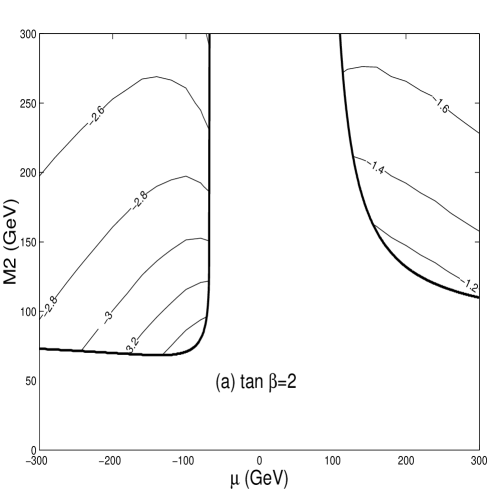
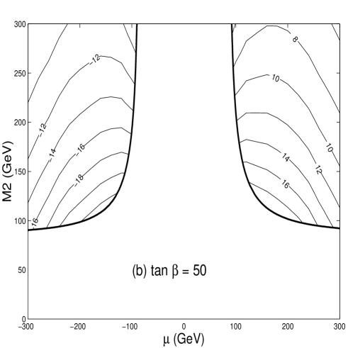
Figure 3: Contour lines of constant WMDM (in units of $10^{-6}$) of the $\tau$ lepton in the $\mu$ vs $M_{2}$ plane for (a) $\tan\beta=2$; (b) $\tan\beta=50$. The thick line in both plots represents the contour $m_{\chi^{\pm}_{1}}=85$ GeV.

Therefore the total result varies between $-1.1.10^{-6}$ and $-1.7.10^{-6}$.

Let’s now turn to the most interesting case of $\mu<0$. Now the chargino/sneutrino and neutralino/stau contributions have the same sign as the non-SUSY one and, therefore, the total result is above the SM prediction. This is shown in the left-hand side of fig. 3(a). As a general feature, $a_{non-SUSY}\sim-2.1~{}.~{}10^{-6}$, whereas $a_{\chi^{\pm}}|_{max}\sim-1.3.10^{-6}$ and $a_{\chi^{0}}\sim-1.10^{-7}$ giving a total WMDM of approximately $-3.5.10^{-6}$ along the line of $m_{\chi^{\pm}_{1}}=85$ GeV. Similarly to the $\mu>0$ case, as the chargino mass increases, its contribution, and therefore in this case $a_{tot}$, decreases reaching a minimum value of $-2.10^{-6}$.

In conclusion, for $\tan\beta=2$ we achieve some enhancement with respect to the SM for $\mu<0$, but not enough to be detected in the near future. Also, as a general feature throughout this analysis, increasing $\tan\beta$ will induce larger WMDM values. This is due to the fact that increasing $\tan\beta$ notably increases the chargino contribution; therefore for $\mu>0$ this will result in a total WMDM of around 0 when $a_{\chi}^{\pm}\sim a_{non-SUSY}$ (which occurs for $\tan\beta\sim 10$), and from then on, in a total WMDM increasingly dominated by the chargino diagrams. For $\mu<0$, as we said all the three contributions to the WMDM (namely non–SUSY, chargino and neutralino) have the same sign, and will always result in a total value bigger than the SM one. This together with the fact that $a_{\chi^{\pm}}$ grows with increasing $\tan\beta$, will lead to values of the WMDM well above the SM contribution from $\tan\beta\sim 10$ onwards.

Let’s focus on $\tan\beta=50$ as the case in which all these effects are maximised. For the same region of parameter space as before, the SM+2HDM is now around $-1.5.10^{-6}$ for $\mu>0$, and a number between $-1.0$ and $-1.7.10^{-6}$ for $\mu<0$ (these variations resulting from the significant increase in the contribution of both the light neutral and the charged Higgs diagrams with respect to the $\tan\beta=2$ case); in the presence of SUSY, we find that now the chargino contribution is totally dominant, being well above both those of the non-SUSY and the neutralino diagrams for both signs of $\mu$. This can be seen in fig. 3(b) which is analogous to fig. 3(a) but for $\tan\beta=50$. As we can see, most of the $\mu<0$ plane and a considerable part of the $\mu>0$ one give a total WMDM for the tau lepton an order of magnitude well above the SM prediction (between $20$ and $6.10^{-6}$ for $\mu>0$, and $-8$ and $-23.10^{-6}$ for $\mu<0$). They correspond to chargino contributions $a_{\chi^{\pm}}\sim(22\rightarrow 7).10^{-6}$ ($\mu>0$) and $a_{\chi^{\pm}}\sim(-20\rightarrow-6.5).10^{-6}$ ($\mu<0$), whereas the corresponding neutralino ones are almost negligible ($|a_{\chi^{0}}|\stackrel{{\scriptstyle<}}{{\sim}}10^{-6}$).

2.2 $(g-2)_{\mu}$

It is interesting to relate these results for the WMDM of the $\tau$ lepton with the analogous calculation of $(g-2)_{\mu}$. This latter case has been extensively studied in the literature, both for the SM [10] and SUSY [11] scenarios, and it is widely motivated by the increasingly good precision of recent and future measurements [12, 13]. As just said, the calculation is totally analogous to that of the previous section, and the formulae can be obtained from the appendix particularizing for the case of having a photon and two muons in the external legs of the different diagrams, which, among other things, allows an analytic solution of the Feynman integrals. We have computed the SUSY contribution to $(g-2)_{\mu}$ for exactly the same spectra for which we computed the WMDMs of the previous section. Imposing a value $|\delta a_{\mu}|\leq 9.10^{-9}$ for the new contributions we find that $\tan\beta\stackrel{{\scriptstyle>}}{{\sim}}10$ is the maximum allowed value for which these spectra respect the bound on $\delta a_{\mu}$. Bigger values of $\tan\beta$ will give rise to unacceptable values of the magnetic moment of the muon. This can be clearly seen in fig. 4, where we plot $\delta a_{\mu}$ in the plane $\mu$ vs $M_{2}$ for (a) $\tan\beta=2$ and (b) $\tan\beta=50$.

 

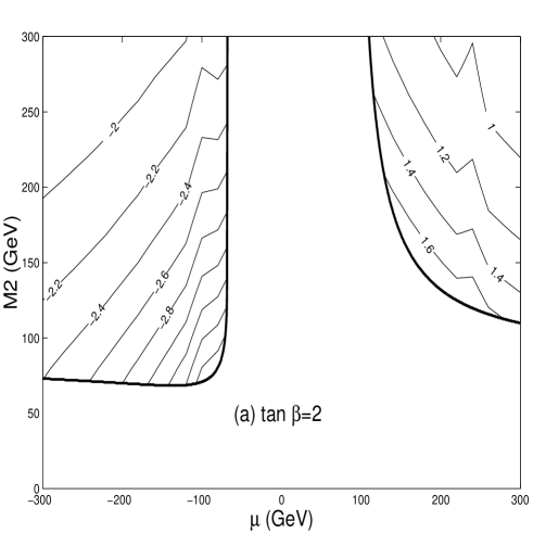
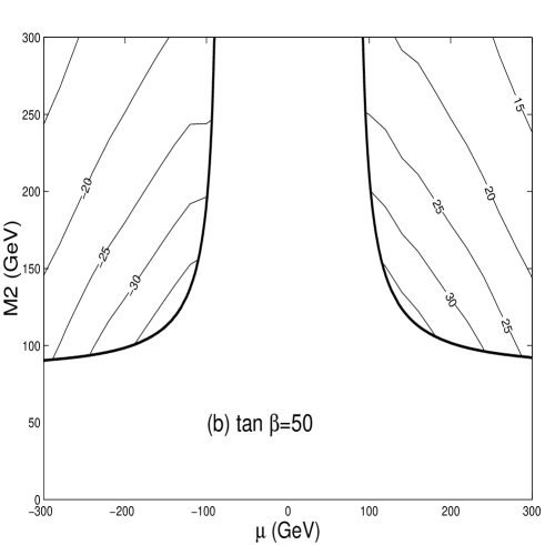
Figure 4: Contour lines of constant $(g-2)$ (in units of $10^{-9}$) of the muon in the $\mu$ vs $M_{2}$ plane for (a) $\tan\beta=2$; (b) $\tan\beta=50$. The thick line in both plots represents the contour $m_{\chi^{\pm}_{1}}=85$ GeV.

As for the WMDM of the $\tau$ lepton, the chargino/sneutrino diagram is the dominant one, therefore it is the variation of $\delta a_{\mu}$ with those masses that is the most interesting one. As mentioned above, we can see that case (b) is totally ruled out by using the experimental bound also given above.

However, these results have been obtained under the assumption of universal soft masses for the three families of squarks and sleptons, that is, in our case $m_{L1}=m_{L2}=m_{L3}$, $m_{E1}=m_{E2}=m_{E3}$. Essentially we are interested in keeping the outstanding predictions for $a_{\tau}$ of the previous section for high values of $\tan\beta$ (over an order of magnitude above the SM result), while maintaning $(g-2)_{\mu}$ under below its experimental bound. Given that in both cases the dominant effect, as $\tan\beta$ increases, is due to the chargino/sneutrino diagram, we may break the degeneracy between the sneutrino masses associated with the different families, in order to achieve the desired result. Therefore we can compute how different these masses have to be (or, in other words, how much bigger $m_{L2}$ has to be with respect to $m_{L3}$) to have a big WMDM for the $\tau$ lepton and an acceptable $(g-2)_{\mu}$.

This can be easily read from fig. 5, where we plot both anomalous magnetic moments vs a generic soft mass, $m_{L}$. The example

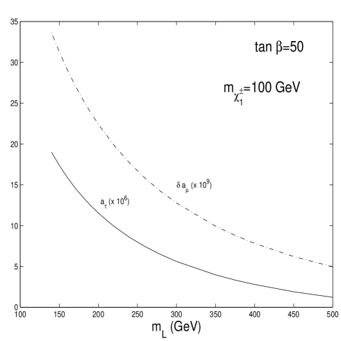
Figure 5: Plot of the WMDM of the $\tau$ lepton (solid line, in units of $10^{-6}$) and of $(g-2)$ of the muon (dot–dashed line, in units of $10^{-9}$) vs a generic slepton soft mass, $m_{L}$, for $\tan\beta=50$.

shown here corresponds to a lightest chargino mass of 100 GeV and $\tan\beta=50$. To obtain a value of $\delta a_{\mu}$ below the limit of $9.10^{-9}$ we have imposed (the most restrictive one) the $m_{L2}$ must be above, approximately, 375 GeV. If we wish to preserve universality of the slepton masses, this in turn would give us a prediction for the WMDM of the $\tau$ lepton of $3.5.10^{-6}$. However keeping $m_{L3}$ at some value between 100 and 200 GeV, while driving $m_{L2}$ to the region of 400 GeV would result in values of $a_{\tau}\sim(1.2-2.0).10^{-5}$, whereas the bounds on $\delta a_{\mu}$ would be fulfilled. In general it will be possible to estimate to what extent this degeneracy has to be broken in order to i) have $a_{\tau}$ as big as possible; ii) maintain $|\delta a_{\mu}|$ below $9.10^{-9}$. The required $\Delta m_{L}\equiv m_{L3}-m_{L2}$ will be a function of $\tan\beta$ and the value of the lightest chargino mass we are picking to evaluate the relevant diagram in both cases.

The main direct effect of such lack of degeneracy of the slepton soft masses would be the existence of non universal corrections to the $Z$–lepton couplings [14]. These non-universal effects are strongly constrained by SLAC and LEP measurements (left-right asymmetries, leptonic widths, $\tau$ polarization data at the Z peak [15], etc.). First indications show that these corrections are never too large in SUSY extensions of the SM, but nevertheless the issue of universality breaking is interesting enough to deserve further investigation.

3 The $b$ quark

Let’s now discuss very briefly the calculation of the WMDM for the case of the $b$ quark. As already pointed out by the authors of ref. [8, 16], the dominant contribution to this calculation comes from the gluon diagram, which is two orders of magnitude bigger than the electroweak ones. Altogether they give a total result of $(3.57-1.95i).10^{-4}$, which will change very little when we plug in the SUSY contributions, which are given in the appendix. In general, the inclusion of the two Higgs doublets will not have a remarkable impact unless we are in a region of high $\tan\beta$ and low pseudoscalar mass $m_{A}$ (for more details, see [8]); therefore we will only discuss the case of $\tan\beta=50$, which on the other hand, maximises the SUSY contributions, which are now given by the diagrams analogous to the chargino and neutralino diagrams discussed for the $\tau$ lepton (with stops and sbottoms, respectively, circulating in the loop) plus a new diagram, a SUSY version of the dominant gluon one, which has gluinos and sbottoms circulating in it.

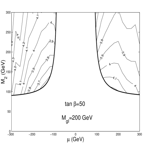
Figure 6: Contour lines of constant WMDM of the $b$ quark (in units of $10^{-4}$) in the $\mu$ vs $M_{2}$ plane, for $\tan\beta=50$ and $M_{g}l=200$ GeV. The thick line in the plot represents the contour $m_{\chi^{\pm}}=85$ GeV.

For $\mu<0$ $a_{non-SUSY}$ deviates from its pure EWSM+QCD value due to the effect of the light Higgs diagram, which increases as the absolute value of $\mu$ does. Therefore we have that $a_{non-SUSY}$ ranges from $3.7.10^{-4}$ to $4.3.10^{-4}$ when we go from $\mu=-100$ GeV to $\mu=-300$ GeV. If, on top of that, we include the effect of SUSY, as is shown in fig. 6, the total value does not change much, because the effect of charginos and neutralinos, which contribute with the same sign, is totally balanced by the gluino diagram which has the opposite sign. $a_{gl}$ ranges between $39$ and $26.10^{-6}$ (for a representative gluino mass of 200 GeV), whereas $a_{\chi^{0}}$ lies between $-11$ and $-26.10^{-6}$, and the chargino contribution is the most variable one, given that it is the chargino mass which is changing on fig. 6: from $-48$ to $3.10^{-6}$.

As for $\mu>0$, $a_{non-SUSY}$ is almost constant at a value of $3.9.10^{-4}$ (the light Higgs diagram is not sensitive to changes in the value of $\mu$ as was also the case with the $\tau$ WMDM); the SUSY diagrams now contribute with opposite signs to the $\mu<0$ case, but there is no exact cancellation between chargino+neutralino diagrams on one hand and the gluino diagram on the other. The final result is then a total real part of the WMDM centered around $a_{non-SUSY}$, being slightly smaller when the chargino contribution decreases (i.e. big values of $M_{2}$ in fig. 6), and slightly bigger when the charginos dominate. As we can read from fig. 6, $3.6.10^{-4}\leq a_{tot}\leq 4.2.10^{-4}$.

Finally, we have verified that, for the considered values of the parameters, the SUSY corrections to $R_{b}$, also induced by these diagrams, are under control.

4 Conclusion

We have presented a full calculation of weak magnetic dipole moments in the framework of the Minimal Supersymmetric Standard Model. In particular we have performed a detailed analysis of the parameter space for the case of the $\tau$ lepton and $b$ quark. For the former we found that the SUSY contributions, in particular those of the diagrams involving charginos and sneutrinos, dominate over the SM result, especially for increasing $\tan\beta$. In general it is perfectly possible to achieve an enhancement of over an order of magnitude with respect to what the SM predicts. This in turn implies a too large contribution of the analogous SUSY diagrams to the calculation of $(g-2)$ of the muon when we assume universal slepton masses; however it is possible in principle to break this degeneracy without affecting any universality–breaking observables and still keep this enhancement for the WMDM of the $\tau$ while having a prediction for $(g-2)_{\mu}$ within the experimental limit.

Note added

After completion of this work we have received the paper of ref. [18] where an independent analysis of the MSSM predictions for the WMDM of the ${\tau}$ lepton and $b$ quark is presented.

Appendix

In this appendix we present the formulae for the supersymmetric contributions to the WMDM of a general, quark or lepton, fermion. As an example, we have depicted in fig. 2 the relevant diagrams involved in the calculation of the WMDM of the tau lepton. A new type of diagram, associated with gluinos, has to be included if we calculate the WMDM of a quark. These diagrams can be expressed as a combination of the scalar, vector and tensor Passarino-Veltman three point functions [17]. We will use instead the parametrization given in [8], which we reproduce here for the sake of completeness. Let $A,B,C$ be the tree particles running into the loop, using the convention shown in fig. 1. Then the relevant integrals are:

$$I_{00;\mu;\mu\nu}\;(p_{-}^{2},(p_{-}+p_{+})^{2},p_{+}^{2},m_{A}^{2},m_{B}^{2},m_{C}^{2}) =$$

$${\displaystyle\int\frac{d^{4}k}{i\pi}}{\displaystyle\frac{\left\{1;k_{\mu},k_{\mu\nu}\right\}}{(k^{2}-m_{A}^{2})\left[(k-p_{-})^{2}-m_{B}^{2}\right]\left[(k+p_{+})^{2}-m_{C}^{2}\right]}}$$

which we will decompose as:

$$\begin{array}[]{rcl}I^{\mu}&=&(p_{-}-p_{+})^{\mu}I_{10}+(p_{-}+p_{+})^{\mu}I_{11}\\ I^{\mu\nu}&=&(p_{+}^{\mu}p_{+}^{\nu}+p_{-}^{\mu}p_{-}^{\nu})I_{21}+(p_{+}^{\mu}p_{-}^{\nu}+p_{-}^{\mu}p_{+}^{\nu})I_{22}+\\ &&(p_{+}^{\mu}p_{+}^{\nu}-p_{-}^{\mu}p_{-}^{\nu})I_{2-1}+g^{\mu\nu}I_{20}\end{array}$$ (A.2)

Let $a^{ABC}$ be the contribution to the WMDM given by this general diagram. Then $a^{ABC}$ will be expressed as a combination of the different $I_{ij}=I_{10},I_{11},I_{21},I_{22},I_{2-1}$ (see for example (A.4)). We omit some of the arguments of the $I_{ij}$s, since the external fermions are on shell. To be more precise, we will use

$$I_{ij}(m_{A},m_{B},m_{C},q)\equiv I_{ij}(p_{-}^{2},(p_{-}+p_{+})^{2},p_{+}^{2},m_{A}^{2},m_{B}^{2},m_{C}^{2})$$ (A.3)

where $p_{-}^{2}=p_{+}^{2}=m^{2}$, with $m$ the mass of the fermion we are considering. We have evaluated both the photon and Z-boson like magnetic dipole moments, $a^{\gamma}$ and $a^{Z}$, fixing $(p_{-}+p_{+})^{2}\equiv q^{2}$ at $0$ and $M_{Z}^{2}$ respectively. Since the only difference, besides the $q$ value, is contained in the coupling of the gauge boson, we will give a unique expression for the two cases.

CHARGINO

Let us first consider the two diagrams associated to the charginos (see fig. 2). The contribution of the chargino-sfermion-sfermion diagram is given by:

$$a^{\chi^{-}ss} = -{\displaystyle\frac{\alpha_{em}}{4\pi}}{\cal S}{\displaystyle\sum_{l=1,2}\;\sum_{i,j=1,2}}{\displaystyle\frac{m}{s^{2}_{W}}}(S_{j1}(x_{s}+y_{s})S^{*}_{i1}+S_{j2}(x_{s}-y_{s})S^{*}_{i2})$$

$$\;\;\;\;\;\;\;\;\;\;\;\;\left[2m\,(\Lambda^{L*}_{jl}\Lambda^{L}_{il}+\Lambda^{R*}_{jl}\Lambda^{R}_{il})\,(I_{10}-I_{21}+I_{22})\right.$$

$$\;\;\;\;\;\;\;\;\;\;\;\;\left.+M_{\chi^{-}_{l}}\,(\Lambda^{R*}_{jl}\Lambda^{L}_{il}+\Lambda^{L*}_{jl}\Lambda^{R}_{il})\,(I_{00}-2I_{10})\right](M_{\chi^{-}_{l}},m_{s}^{j},m_{s}^{i},q)\,.$$

The SUSY particles running in the loop are given in the mass basis, so the usual matrices relating mass and interaction states (for both charginos and sfermions) will appear in the vertices. In particular, $S_{i\alpha}$ is the corresponding rotation matrix for the sfermions involved in the loop. The subscript $l$ labels the two charginos. The matrices $\Lambda^{R,L}$ mainly describe the chargino-sfermion-sfermion vertex. For stop-like squarks (i.e., $T_{3}^{s}=1/2$), they are given by

$$\begin{array}[]{rcl}\Lambda^{L}_{il}&=&-{\displaystyle\frac{m_{d}}{\sqrt{2}M_{W}\cos\beta}}T_{i1}U_{l2}\\[14.22636pt] \Lambda^{R}_{il}&=&T_{i1}V^{*}_{l1}-{\displaystyle\frac{m_{u}}{\sqrt{2}M_{W}\sin\beta}}T_{i2}V^{*}_{l2}\;\;,\end{array}$$ (A.5)

with $S_{i\alpha}=T_{i\alpha}$, and for sbottom-like squarks ($T_{3}^{s}=-1/2$)

$$\begin{array}[]{rcl}\Lambda^{L}_{il}&=&B_{i1}U^{*}_{l1}-{\displaystyle\frac{m_{d}}{\sqrt{2}M_{W}\cos\beta}}B_{i2}U^{*}_{l2}\\[14.22636pt] \Lambda^{R}_{il}&=&-{\displaystyle\frac{m_{u}}{\sqrt{2}M_{W}\sin\beta}}B_{i1}V_{l2}\;\;,\end{array}$$ (A.6)

where $S_{i\alpha}=B_{i\alpha}$. The matrices $U,V$ in the previous equations are the usual ones that allow expression of the two chargino mass eigenstates as a combination of the wino and charged higgsino. These expressions are trivially generalized for sleptons, by just replacing $m_{u}$ by $m_{l}$ and setting $m_{d}=0$.

The coupling of the gauge boson $(Z,\gamma)$ to the sfermions is parametrized by

$$x_{s}=\left[\begin{array}[]{c}{\displaystyle\frac{1}{2s_{W}c_{W}}}(T_{3}^{s}-2Q_{s}s^{2}_{W})\\[8.53581pt] Q_{s}\end{array}\right]\;\;\;y_{s}=\left[\begin{array}[]{c}{\displaystyle\frac{T_{3}^{s}}{2s_{W}c_{W}}}\\[8.53581pt] 0\end{array}\right]$$ (A.7)

Finally, ${\cal S}$ stands for a global factor $2T_{3f}=\pm 1$.

The contribution of the sfermion-chargino-chargino diagram is given by:

$$a^{s\chi^{-}\chi^{-}} = -{\displaystyle\frac{\alpha_{em}}{4\pi}}{\displaystyle\sum_{i=1,2}\;\sum_{l,m=1,2}}{\displaystyle\frac{m}{s_{W}^{2}}}\left[2m({\Lambda}^{L*}_{im}{\cal O}^{R}_{ml}{\Lambda}^{L}_{il}+{\Lambda}^{R*}_{im}{\cal O}^{L}_{ml}{\Lambda}^{R}_{il})(I_{10}-I_{21}+I_{22})\right.$$

$$\;\;\;\;\;\;\;\;\;\;\left.+M_{\chi^{-}_{l}}({\Lambda}^{R*}_{im}{\cal O}^{L}_{ml}{\Lambda}^{L}_{il}+{\Lambda}^{L*}_{im}{\cal O}^{R}_{ml}{\Lambda}^{R}_{il})(I_{10}-I_{11})\right.$$

$$\;\;\;\;\;\;\;\;\;\;\left.+M_{\chi^{-}_{m}}({\Lambda}^{R*}_{im}{\cal O}^{R}_{ml}{\Lambda}^{L}_{il}+{\Lambda}^{L*}_{im}{\cal O}^{L}_{ml}{\Lambda}^{R}_{il})(I_{10}+I_{11})\right](m_{s}^{i},M_{\chi^{-}_{m}},M_{\chi^{-}_{l}},q)$$

where the matrices

$${\cal O}^{L}_{ml}=\left[\begin{array}[]{c}{\displaystyle\frac{1}{s_{W}c_{W}}}(c^{2}_{W}\delta_{ml}-\frac{1}{2}V_{m2}V^{*}_{l2})\\[8.53581pt] \delta_{ml}\end{array}\right]\;\;\;{\cal O}^{R}_{ml}=\left[\begin{array}[]{c}{\displaystyle\frac{1}{s_{W}c_{W}}}(c^{2}_{W}\delta_{ml}-\frac{1}{2}U^{*}_{m2}U_{l2})\\[8.53581pt] \delta_{ml}\end{array}\right]$$ (A.9)

describe, up to some factor, the $(Z,\gamma)-\chi^{+}-\chi^{-}$ vertex.

NEUTRALINO

The corrections induced by neutralinos are parametrized in a similar way. In particular, the contribution of the neutralino-sfermion-sfermion diagram can be written as:

$$\begin{array}[]{rcrl}a^{\chi^{0}ss}&=&{\displaystyle\frac{\alpha_{em}}{4\pi}}{\displaystyle\sum_{l=1,4}\;\sum_{i,j=1,2}}&2m\,(S_{j1}(x_{s}+y_{s})S^{*}_{i1}+S_{j2}(x_{s}-y_{s})S^{*}_{i2})\\[11.38109pt] &&&\left[2m({\Lambda}_{jl}^{L*}{\Lambda}_{il}^{L}+{\Lambda}_{jl}^{R*}{\Lambda}_{il}^{R})(I_{10}-I_{21}+I_{22})\right.\\[8.53581pt] &&&\left.+M_{\chi^{0}_{l}}({\Lambda}_{jl}^{R*}{\Lambda}_{il}^{L}+{\Lambda}_{jl}^{L*}{\Lambda}_{il}^{R})(I_{00}-2I_{10})\right](M_{\chi^{0}_{l}},m_{s}^{j},m_{s}^{i},q)\,.\end{array}$$ (A.10)

where now

$$\begin{array}[]{rcl}\Lambda^{L}_{il}&=&\phantom{-}T_{i1}\left[Q_{u}N^{\prime*}_{l1}+{\displaystyle\frac{(v+a)_{u}}{2s_{W}c_{W}}}N^{\prime*}_{l2}\right]+T_{i2}{\displaystyle\frac{m_{u}}{2M_{W}s_{W}\sin\beta}}N^{*}_{l4}\\[14.22636pt] \Lambda^{R}_{il}&=&-T_{i2}\left[Q_{u}N^{\prime}_{l1}+{\displaystyle\frac{(v-a)_{u}}{2s_{W}c_{W}}}N^{\prime}_{l2}\right]+T_{i1}{\displaystyle\frac{m_{u}}{2M_{W}s_{W}\sin\beta}}N_{l4}\end{array}$$ (A.11)

for stop-like sfermions running in the loop, and

$$\begin{array}[]{rcl}\Lambda^{L}_{il}&=&\phantom{-}B_{i1}\left[Q_{d}N^{\prime*}_{l1}+{\displaystyle\frac{(v+a)_{d}}{2s_{W}c_{W}}}N^{\prime*}_{l2}\right]+B_{i2}{\displaystyle\frac{m_{d}}{2M_{W}s_{W}\cos\beta}}N^{*}_{l3}\\[14.22636pt] \Lambda^{R}_{il}&=&-B_{i2}\left[Q_{d}N^{\prime}_{l1}+{\displaystyle\frac{(v-a)_{d}}{2s_{W}c_{W}}}N^{\prime}_{l2}\right]+B_{i1}{\displaystyle\frac{m_{d}}{2M_{W}s_{W}\cos\beta}}N_{l3}\end{array}$$ (A.12)

for diagrams involving sbottom-like sfermions. In these equations, $v=T_{3}-2Qs^{2}_{W}$, $a=T_{3}$ and $N$ are the rotation matrices that relate mass eigenstate neutralinos to the photino, wino and neutral higgsinos.

The sfermion-sfermion-neutralino diagram only contributes to $a^{Z}$ and is given by

$$a^{s\chi^{0}\chi^{0}} = {\displaystyle\frac{\alpha_{em}}{4\pi}}{\displaystyle\sum_{i=1,2}\;\sum_{l,m=1,4}}{\displaystyle\frac{2m}{s_{W}c_{W}}}\left[2m({\Lambda}^{L*}_{im}{\cal O}^{R}_{ml}{\Lambda}^{L}_{il}+{\Lambda}^{R*}_{im}{\cal O}^{L}_{ml}{\Lambda}^{R}_{il})(I_{10}-I_{21}+I_{22})\right.$$

$$\;\;\;\;\;\;\;\;\left.+M_{\chi^{0}_{l}}({\Lambda}^{R*}_{im}{\cal O}^{L}_{ml}{\Lambda}^{L}_{il}+{\Lambda}^{L*}_{im}{\cal O}^{R}_{ml}{\Lambda}^{R}_{il})(I_{10}-I_{11})\right.$$

$$\;\;\;\;\;\;\;\;\left.+M_{\chi^{0}_{m}}({\Lambda}^{R*}_{im}{\cal O}^{R}_{ml}{\Lambda}^{L}_{il}+{\Lambda}^{L*}_{im}{\cal O}^{L}_{ml}{\Lambda}^{R}_{il})(I_{10}+I_{11})\right](m_{s}^{i},M_{\chi^{0}_{m}},M_{\chi^{0}_{l}},q)\,.$$

where

$$\begin{array}[]{rcl}{\cal O}^{L}_{ml}&=&-\frac{1}{2}N_{m3}N^{*}_{l3}+\frac{1}{2}N_{m4}N^{*}_{l4}\\[8.53581pt] {\cal O}^{R}_{ml}&=&-{\cal O}^{L*}_{ml}\end{array}$$ (A.14)

are the matrices describing the $Z-\chi^{0}-\chi^{0}$ vertex. All these expressions are also valid for the WMDM of leptons, just making the replacements we suggested above.

GLUINO

Finally, we have to consider the gluino diagram in the evaluation of the WMDM of quarks. This diagram is similar to the neutrino-sfermion-sfermion one. We get:

$$a^{\tilde{g}ss} = {\displaystyle\frac{\alpha_{s}}{4\pi}}{\displaystyle\sum_{i,j=1,2}}C_{R}\,2m\,(S_{j1}(x_{s}+y_{s})S^{*}_{i1}+S_{j2}(x_{s}-y_{s})S^{*}_{i2})$$

$$\;\;\;\;\;\;\;\;\left[2m\,\delta_{ij}\,(I_{10}-I_{21}+I_{22})-M_{\tilde{g}}\,(S_{i2}S^{*}_{j1}+S_{i1}S^{*}_{j2})\,(I_{00}-2I_{10})\right](M_{\tilde{g}},m_{s}^{j},m_{s}^{i},q)\,.$$

where $C_{R}=4/3$ and $\alpha_{s}\equiv\alpha_{s}(M_{Z})=0.118$.

The previous expressions can be simplified when considering $a^{\gamma}$. Firstly, some of the diagrams do not contribute. Secondly, since the $U(1)_{em}$ is unbroken, the photon coupling is of course diagonal in the sfermion and chargino indices. On the other hand, the $I_{ij}$ are reduced to well known analytical functions when $q=0$ and $m_{B}=m_{C}$. To be more precise, the following relations hold:

$$I_{11}(m,M,M,q) = 0$$

$$I_{10}(m,M,M,0) = -{\displaystyle\frac{1}{4M^{2}}}\left[(1-3x)(1-x)^{-2}-2x^{2}(1-x)^{-3}\ln x\right]$$

$$[I_{10}-I_{21}+I_{22}](m,M,M,0) = -{\displaystyle\frac{1}{12M^{2}}}\left[(1-5x-2x^{2})(1-x)^{-3}-6x^{2}(1-x)^{-4}\ln x\right]$$

$$[I_{00}-2I_{10}](m,M,M,0) = -{\displaystyle\frac{1}{2M^{2}}}\left[(1+x)(1-x)^{-2}+2x(1-x)^{-3}\ln x\right]$$ (A.16)

where $x=(\frac{m}{M})^{2}$. Then, the well known results for $(g-2)_{\mu}$ in SUSY models can be recovered as a particular and simple case in our general calculation.

References

-
[1]
For reviews see for example H.P. Nilles, Phys. Rep.
110 (1984) 1;
H.E. Haber and G.L. Kane, Phys. Rep. 117 (1985) 75. -
[2]
T.G. Rizzo,
Phys. Rev. D51 (1995) 3811 and hep-ph/9704337;
G. Köpp, D. Schaile, M. Spira and P.M. Zerwas, Z. Phys. C65 (1995) 545. - [3] A. Böhm, L3 Collaboration, talk presented at the Rencontres de Moriond, Electroweak Interactions and Unified Theories, Les Arcs, France, 15–22 March, 1997.
-
[4]
See, for example, C. Artz, M.B. Einhorn and J. Wudka,
Phys. Rev. D49 (1994) 1370;
R. Escribano and E. Massó, Nucl. Phys. B429 (1994) 19 and Phys. Lett. B395 (1997) 367. - [5] J. Bernabéu, G.A. González-Sprinberg, and J. Vidal, Phys. Lett. B326 (1994) 168.
- [6] E. Sánchez, Fourth International Workshop on Tau Lepton Physics, Estes Park, Colorado, 16–19 September 1996.
- [7] J. Bernabéu, G.A. González-Sprinberg, M. Tung and J. Vidal, Nucl. Phys. B436 (1995) 474.
- [8] J. Bernabéu, D. Comelli, L. Lavoura and J.P. Silva, Phys. Rev. D53 (1996) 5222.
-
[9]
Glen Cowan, ALEPH Results at 172 GeV;
François Richard, DELPHI Results at 172 GeV;
Marco Pieri, L3 Physics Results at 172 GeV LEP Run;
Sachio Komamiya, Preliminary OPAL Results at 170 & 172 GeV;
CERN PPE Seminar, 25 February 1997.
CDF Collaboration, FERMILAB-PUB-97/031-E, Submitted to Phys. Rev. D;
D0 Collaboration, Phys. Rev. Lett. 75 (1995) 618. -
[10]
T. Kinoshita, Phys. Rev. Lett. 75 (1995) 4728;
A. Czarnecki, B. Krause and W.J. Marciano, Phys. Rev. Lett. 76 (1996) 3267;
S. Laporta and E. Remiddi, Phys. Lett. B379 (1996) 283;
F. Jegerlehener, Nucl. Phys. Proc. Supl. 51C (1996) 131-141. -
[11]
J.P. Leveille, Nucl. Phys. B137 (1978) 63;
S.A. Abel, W.N. Cottingham and I.B. Whittingham, Phys. Lett. B259 (1991) 307;
J.L. López, D.V. Nanopoulos and X. Wang, Phys. Rev. D49 (1994) 366;
U. Chattopadhyay and P. Nath, Phys. Rev. D53 (1996) 1648;
T. Moroi, Phys. Rev. D53 (1996) 6565;
M. Carena, G.F. Giudice and C.E.M. Wagner, Phys. Lett. B390 (1997) 234. - [12] Particle Data Group, R.M. Barnett et al., Phys. Rev. D54 (1996) 1.
- [13] V.W. Hughes, in Frontiers of High Energy Spin Physics edited by T. Hasegawa et al. (Universal Academy Press, Tokyo, 1992), pp. 717-722.
- [14] J. Bernabéu and A. Pilaftsis, Phys. Lett. B351 (1995) 235.
- [15] A. Pich, Fourth International Workshop on Tau Lepton Physics, Estes Park, Colorado, 16–19 September 1996, hep-ph/9612308.
- [16] J. Bernabéu, G.A. González-Sprinberg and J. Vidal, Phys. Lett. B397 (1997) 255.
- [17] G. Passarino and M. Veltman, Nucl. Phys. B160 (1979) 151.
- [18] W. Hollik, J.I. Illana, S. Rigolin and D. Stöckinger, preprint KA-TP-11-1997, DFPD/97/28, hep-ph/9707437.