RU-97-22

Abstract: Not yet. ALEPH’s recent exclusion limit employs an aggressive determination of theoretical uncertainties using a simplified application of the Bayesian method. The validity of their analysis can be evaluated by its further implications, such as contradicting the existence a b quark and requiring relations between hadronic event-shape observables which are not observed. Traditional error estimation methods result in a much larger estimate for the theoretical uncertainties. This puts the ALEPH and also Csikor-Fodor limits at the $\sim 1~{}\sigma$ level for the very light gluino scenario. A recent astrophysical result implies direct searches will be more difficult than previously anticipated, adding to the importance of reducing the QCD uncertainty in predictions sensitive to indirect effects of light gluinos. Some possible indications in favor of a light gluino are noted.

All the LEP experiments have addressed the question of constraining QCD color factors by high-statistics data on hadronic event shapes in $Z^{0}$ decay. See, e.g., [1, 2, 3, 4] and references therein. The agreement with QCD is entirely adequate, but the sensitivity to the effective number of flavors has not been sufficient up to now to rule out the presence of a light gluino which would increase the effective number of flavors from $\sim 5$ to $\sim 8$. The strategy of the new ALEPH analysis[4] is to fit both 4-jet angular distributions and the differential 2-jet rate to simultaneously constrain $\alpha_{s}(m_{Z})$ and $n_{f}$, the effective number of flavors. Since every hadronic event contributes to the differential two jet rate, it is well-determined statistically. It is a first-order observable, i.e., its leading contribution is $O(\alpha_{s})$, so it is sensitive to the running of $\alpha_{s}$. Thus it feels $n_{f}$ through the coefficient of the $\beta$ function, $b_{0}=\frac{11}{6}\frac{C_{A}}{C_{F}}-\frac{2}{3}n_{f}\frac{T_{F}}{C_{F}}$. The various 4-jet angular distributions are second-order variables, i.e., at the parton level their leading contribution is $O(\alpha_{s}^{2})$. Particular angular correlations enhance the sensitivity to 4-fermion final states in comparison to the dominant $q\bar{q}gg$ final states. However 4-jet angular distributions are less precisely determined statistically than is the differential 2-jet rate. The nice observation of ALEPH is that the shapes of the error ellipses from the two types of measurements tend to be complementary, so combining the constraints could produce a more precise determination than either one alone. The final result quoted by ALEPH from this analysis is[4]: $\alpha_{s}(m_{Z})=0.1162\pm 0.0012(stat)\pm 0.0040(syst)$ and $n_{f}=4.24\pm 0.29(stat)\pm 1.15(syst)$. The crucial question is whether their estimate of the systematic uncertainty is realistic or overly optimistic.

The fundamental issue is ALEPH’s approach to assigning quantitative systematic error bars. For each source of systematic uncertainty considered, several variations on the model are fit to the data, resulting in a determination of $\alpha_{s}(m_{Z})$ and $n_{f}$, with some $\chi^{2}$ for the fit. They adopt what they characterize as a “Bayesian point of view”, which they describe as follows[4]: “The Bayesian idea is that a priori all models can be considered equally well suited for usage in the analysis, but from a bad $\chi^{2}$ it is deduced that the a posteriori probability of such a model is low, and therefore this model should get a small weight when estimating the actual systematic error. …the systematic error corresponds to the increase in $\chi^{2}$ by one.” If all possible models, or at least a complete unbiased sample of models is explored by the analysis, the above ansatz should be valid on average over many experimental fits. The question which must be addressed is whether the ansatz remains valid when restricted to the class of model variations considered by ALEPH.

It is intuitively plausible that when data are being modeled from first principles with a correct theory, and only the parameters of the theory require specification, that the prescription outlined above would give a correct estimation of errors. Moving away from this ideal but rarely realized case, one may have a situation in which the form of some model function is known theoretically (e.g., the power-dependence of pseudoscalar meson masses on the light-quark mass in the $m_{q}\rightarrow 0$ limit of a lattice gauge theory calculation) and only some parameters of the function are unknown. Here it is also possible to rely on the Bayesian analysis as described above, for aspects of the modeling which refer to the known functional form.

However in the situation most commonly encountered in practice, the form of functions appearing in the model are not known from first principles. Examples are the functional forms which are used to describe parton distribution functions or parton hadronization. When, as is usually the case, functional forms are chosen for simplicity and convenience, and parameters tuned to fit a diverse collection of data, naive application of the Bayesian approach can lead to a completely wrong estimate of the actual theoretical uncertainty. A recent case in point is the production of high $p_{\perp}$ jets observed by CDF which was anomalously large in comparison to predictions of QCD with the then-standard gluon distribution functions[7]. With the standard functional form of the gluon distribution function, the QCD prediction seemed very strongly constrained by other data. However only a mild generalization of the form was needed to fit all data including the high-$p_{\perp}$ jets[8].

The most difficult situation of all is when one must model both the conventional theory and the theory with some new degree of freedom. In this case, to completely survey the model space as required for a correct analysis, requires modeling and fitting all the physical observables used to constrain the models, with and without the new degree of freedom. Here, since the form and parameters of hadronization models are tuned to agree with an enormous body of data, the correct application of Bayesian principles minimally requires generalizing Herwig and JETSET to include light gluinos and varying all the parameters of the hadronization models to fit all data. To the extent that the underlying physics (e.g., non-perturbative QCD) is well or poorly understood, the generalization of the modeling to new degrees of freedom will or will not provide an adequate framework for the Bayesian analysis.

In addition to these non-perturbative issues, the perturbative QCD predictions at the parton level depend on the renormalization scale $\mu$, the matching scheme used to obtain resummed predictions, and also on the parameter $y_{cut}$ and scheme used to define 4-jet events. The problem of fully exploring the model dependence associated with these parameters is discussed below.

Given that the full implementation of the Bayesian approach is so demanding, we can ask whether it might still be valid in practice when applied in the simplified way adopted by ALEPH. Independent experimental evidence will allow us to answer this question.

Three sources of uncertainty dominate the ALEPH estimate of their systematic error:

• The uncertainty in the theoretical prediction for $D_{2}$, the differential 2-jet rate, due to sensitivity to renormalization scale, $\mu$.

• The uncertainty in the theoretical prediction for $D_{2}$ due to sensitivity to uncontrolled aspects of the resummation of large logarithms of $y_{3}$.

• The modeling of the hadronization of the partons.

Two other uncertainties in the theoretical predictions which may be important but which were not considered are:

• The uncertainty in the theoretical prediction for the 4-jet angular distributions due to sensitivity to renormalization scale, $\mu$.

• The uncertainty in the theoretical prediction for the 4-jet angular distribution due to large logarithms of $y_{cut}$, i.e., the dependence of the theoretical prediction on jet definition.

Two schemes for treating the effects of subleading logarithms of $y_{3}$ in the prediction for the differential 2-jet rate were considered, R matching and log-R matching. If subleading logs and higher order corrections are unimportant, the schemes should give identical results and should exhibit only weak scale dependence. Fig. 1 from [4] shows their fit results for the two schemes, along with the $\chi^{2}$ for each fit, as a function of $lnf\equiv ln(\mu^{2}/m_{Z}^{2})$. It can be seen that the extracted value of $n_{f}$ is sensitive to $\mu$, in both schemes. Since $n_{f}$ is a physical quantity, it cannot depend on $\mu$ or scheme.

If one knew that the true prediction for the functional dependence on $y_{3}$ of the differential 2-jet distribution were given by the functional dependence predicted by one of the schemes, for some particular value of $\mu$, then one could obtain the uncertainty associated with the $\mu$ dependence by the Bayesian prescription, and would get the correct mean value of the physical parameters by using the scheme and $\mu$ value with the smallest $\chi^{2}$. ALEPH assumes this is the case and takes the 1-sigma “theoretical error” (scale uncertainty) to be⁴ (c.f., formulae (15,16) of ref. [4])

$$\Delta^{th}n_{f}=C~{}{\rm max}_{[i]}\left(\frac{|n_{f}^{[i]}-n_{f}^{*}|}{\sqrt{{\rm max}(1,|\chi^{2}_{*}-\chi^{2}_{[i]}|)}}\right)~{}~{};~{}~{}C={\rm max}\left(1,\sqrt{\chi^{2}_{*}/N_{dof}}\right).$$ (1)

$i$ labels the fit parameters of various models, with $*$ designating the best fit. Table 1, taken from Table 3 of ref. [4], shows for the two schemes the best-fit and $\Delta\chi^{2}=\pm 1$ fits. Rather than treating $i$ as a continuous variable regarding the $\mu$ dependence shown in Fig. 1, they only consider the discrete choices listed in Table 1; applying eqn (1), they find $\Delta^{th}=1.01$.

The best fit (log R matching with $lnf=-1.3$) gives $n_{f}=3.68$. However ALEPH averages the best-fit results of the log R and R matching schemes and quotes $n_{f}=4.24\pm 1.01(th)\pm 0.45(had)\pm 0.27(de)\pm 0.29(stat)$.

Table 1: Scheme and scale variations in ALEPH Fit B analysis, $N_{dof}=73$.

Variations	$\rm\alpha_{s}(M_{Z})$	$n_{f}$	$\chi^{2}$	$\mu/M_{Z}$
Theoretical Prediction
nominal: $\log$R, ln $f=-$1.3	0.1154	3.68	78.5	0.52
$\log$R, ln $f=-$1.8	0.1182	4.08	79.8	0.41
$\log$R, ln $f=-$0.6	0.1130	3.09	79.6	0.74
$R$, ln $f=-$0.5	0.1210	5.81	83.3	0.78
$R$, ln $f$ = 0.0	0.1175	4.88	81.6	1.00
$R$, ln $f$ = 0.7	0.1141	3.57	83.0	1.42

The traditional prescription for estimating the $\pm 1\sigma$ systematic error from scale uncertainty is to take it to be the range of $n_{f}$ obtained by varying $\mu/\sqrt{s}$ over the range [1/2,2], i.e., $lnf$ between $\pm 1.4$. From Fig. 1 this gives $n_{f}=4.88\pm 2.5(th)$, for the R-matching scheme, and $n_{f}=2.7\pm 1(th)$ for the logR scheme. The conservative conclusion is that the dependence of measured distributions on $n_{f}$ is sensitive to truncation of the perturbation series (reflected in the sensitivity to $\mu$) and also to subleading logarithms of $y_{3}$ (reflected in the sensitivity to matching scheme) and therefore one cannot draw strong conclusions until the theoretical predictions are improved.

Fortunately, we have two pieces of independent empirical evidence to test the validity of ALEPH’s more aggressive estimate of the scale and resummation scheme uncertainty.

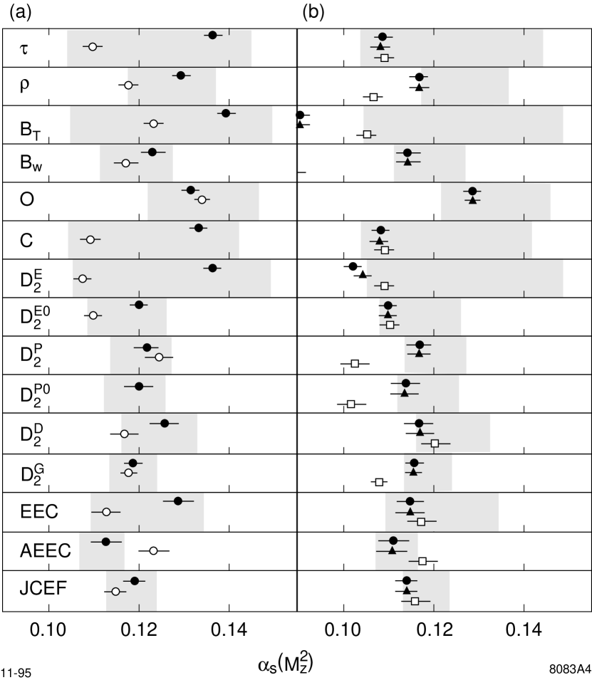
Figure 2: (a) values of $\alpha_{s}(m_{Z})$ from QCD fits to various event shape distributions using “physical” ($\mu=M_{Z}$) – solid circles – and experimentally-optimized scales – open circles. For each observable the shaded region indicates the total uncertainty estimated in Ref. [11], dominated by the contribution from wide variation of the renormalization scale. (b) shows similar comparisons for other scale-setting prescriptions: Principle of Minimal Sensitivity (solid circles), Fastest Apparent Convergence (solid triangles) and Brodsky-Lepage-Mackenzie (open squares). Taken from ref. [10].

First of all, consider the procedure for fixing the scale uncertainty. As noted above, the underlying assumption is that there is some value of $\mu$ for which the net effect of neglected higher orders and subleading logs is minimal so that the functional dependence of the predicted distribution on $y_{3}$ gives a good representation of the complete result. This amounts to the principle of experimental optimization: fixing $\mu$ to the value $\mu=\mu_{\rm EO}$ which minimizes $\chi^{2}$ for that observable. Unless the differential two-jet rate is a lucky accident, the same principle should apply to any event-shape distribution (e.g., thrust, energy-energy correlation, etc). If using $\mu_{\rm EO}$ does in fact subsume the effects of neglected terms, the values of $\alpha_{s}(m_{Z})$ obtained from different event shape distributions, each at its own $\mu_{\rm EO}$, should be the same up to statistical and systematic errors other than those associated with scale uncertainty. Burrows has analyzed various scale-fixing proposals[10] and finds that the dispersion of values of $\alpha_{s}(m_{Z})$ obtained with the experimentally-optimized-scale prescription is no better than the dispersion from other scale-fixing prescriptions, as evident in Fig. 2 from ref. [10] reproduced here. That study used $O(\alpha_{s}^{2})$ rather than resummed predictions. However from Figs 34-37 of ref. [11] one can see that the dispersion in $\alpha_{s}(m_{Z})$ determinations using $\mu_{EO}$ is large in this case as well, even restricting to matching schemes and observables for which $\chi^{2}/N_{dof}\leq 1$. Thus it is not true that the effects of neglected higher order corrections are effectively included by choosing the $\mu$ which minimizes $\chi^{2}$.

Next consider the problem of resummation scheme ambiguity. The log-R matching scheme gives the best-fit, with a $\chi^{2}$ of 78.5 compared to $81.6$ from the R-matching scheme. Therefore, if the Bayesian procedure were being consistently implemented, the log-R matching scheme would be a posteriori identified as the model which gives the best estimate of the physical parameters. Within the set of models considered by ALEPH, their analysis procedure thus gives $n_{f}=3.68\pm 0.29(stat)\pm 1.15(syst)$ as discussed above. The $\pm 0.29$ statistical error means that repeating the experiment many times will yield a value of $n_{f}$ in the range 2.93-4.42 in 99% of the trials. The log-R matching scheme prediction simply does not tolerate $n_{f}>4.5$, for any $\mu$, as apparent from Fig. 1. Thus strictly following Bayesian reasoning[6] requires reject the log R matching scheme for the $D_{2}$ observable because it contradicts our a priori knowledge that $n_{f}\geq 5$. This phenomenon illustrates that Bayesian reasoning can only be applied safely when all relevant experimental information is included in the fit and a sufficiently complete set of theoretical models is being fit. Otherwise, one can wind up in a local rather than global minimum in the space of possible models.

Hadronization errors are similarly not amenable to the Bayesian method, unless much more general hadronization models are used. In particular, the parton shower modeling must include light gluinos and the hadrons containing them, if one is to consistently determine whether a model with light gluinos can fit the data. In the absence of such an undertaking, one can apply the traditional method of trying various hadronization models and seeing if the resultant values of $n_{f}$ change. OPAL[1] investigated the effect on 4-jet angular distributions of changing parameters in a given hadronization model by $O(10\%)$ and found it produced shifts in $n_{f}$ of order 1 unit (see Table 1 of [1]). ALEPH did not try changing parameters in a given hadronization model, but reports that using Herwig rather than JETSET to model the differential 2-jet rate leads to a best-fit value of $n_{f}=6.21$ with only a slight loss of fit quality ($\chi^{2}/N_{dof}$ increases from $81.6/73=1.12$ to $91.6/73=1.25$). The fact that such a large shift in $n_{f}$ accompanies a change of model should have been followed up by varying $\mu$ and changing matching scheme, to discover the best fit which can be obtained with the new hadronization model.

A final area where there may be additional theoretical uncertainty which cannot yet be quantified is the question of the sensitivity of the 4-jet distributions to the scale $\mu$ and to details of the jet definition ($y_{cut}$ and scheme). The 1-loop correction to 4-jet matrix elements was not available when the ALEPH analysis was started. However it has recently been determined[12] and the correction to the angular dependence is small. This can be seen in Fig. 3 from ref. [13] which shows the Bengtsson-Zerwas angular distribution at tree level and 1-loop for $n_{f}=5$ and at 1-loop for $n_{f}=8$, compared to ALEPH data. Since 1-loop corrections to the angular distributions are small, $\mu$ dependence of the angular distribution is evidently not a problem. At the same time, Fig. 3 illustrates that light gluinos make only a very small change in the angular distribution, which is why the $n_{f}$ extraction is so sensitive to corrections to the perturbative prediction.

No resummed calculation exists for the 4-jet angular distributions, but the effects of resummation may be large. First of all, L3 found considerable sensitivity to $y_{cut}$ in their color factor analysis[3]. Secondly, differential distributions such as $D_{2}$ which depend on defining jets, for which the $y_{cut}$ dependence has been determined, display a significant sensitivity to $y_{cut}$. Finally, the sensitivity of $n_{f}$ to hadronization model shows that low $p_{t}$ aspects of the distribution of hadrons relative to the jets affect the angular distribution. Thus soft and colinear gluon radiation may modify the angular dependence found in a fixed order calculation.

It is desirable to estimate what result ALEPH would have reported had traditional error estimation methods of earlier experiments[1, 2, 3] been used. We can only give a lower bound on the systematic error, since ALEPH did not check the sensitivity of its $n_{f}$ extraction to variation of the parameters of the hadronization model or choice of $y_{cut}$ for the 4-jet angular distributions, while the former made a significant contribution to, e.g., the OPAL error[1]. We must use R matching, since the log R matching scheme is excluded because it contradicts the existence of the b quark. We take $\sigma^{th}=2.5$ because this reproduces the $n_{f}$ range obtained for $1/2<\mu/M_{Z}<2$. Combining quadratically with the $\pm 0.45(had)\pm 0.27(de)\pm 0.29(stat)$ obtained by ALEPH, gives $n_{f}=4.88\pm 0.29(stat)\pm 2.57(syst)$. Using the PDG prescription for obtaining limits when part of the experimental range is unphysical ($n_{f}<5$), this implies the 95% cl limit $n_{f}\leq 9.95$, or the 77% cl limit $n_{f}\leq 8$.

It is interesting that the $\pm 2.57(syst)$ obtained from the ALEPH combined fit to $D_{2}$ and the 4-jet angular distributions by traditional uncertainty estimation procedures is actually a larger than obtained using the 4-jet angular distributions alone[1, 2, 3]. The reason for this is that $D_{2}$ is actually very sensitive the $\mu$, even after resummation, while the 4-jet angular distribution is not, so that the ALEPH combined analysis only results in a more precise determination of $n_{f}$ if the $\mu$ range can be limited. However the results of ref. [10] show that ALEPH’s attempt to limit the $\mu$ range by embracing the “experimental optimization” prescription is not valid.

Csikor and Fodor (CF) receintly studied the effect of light gluinos on the running of $\alpha_{s}(Q^{2})$[14]. By restricting themselves to $\alpha_{s}$ extracted via 3-loop perturbative predictions for $R_{had}$ in $\tau$ decay and in $e^{+}e^{-}$ collisions at the $Z^{0}$ and below, they largely avoid the hadronization and scale uncertainties of the hadronic event shape analyses. The fit is mainly constrained by the values $\alpha_{s}(m_{\tau})=0.335\pm 0.053$ and $\alpha_{s}(m_{Z})=0.123\pm 0.006$ because the data at intermediate values of $Q$ are statistically much weaker. However the error on $\alpha_{s}(m_{\tau})$ has been argued[15] to be of order twice as large as used by CF. Thus in their final analysis for the very light gluino case, CF do not use $\alpha_{s}(m_{\tau})$ at all. They find a very light gluino is disfavored only at about 70% cl. The 99.97% cl limit they quote after combining with the ALEPH limit mainly reflects the ALEPH number, which we have argued underestimates the theoretical uncertainty and does not correctly deal with the manifestly unphysical log R matching. Modifying the ALEPH result to $n_{f}=4.88\pm 0.29(stat)\pm 2.57(syst)$, as obtained using standard methods of error estimation, leads to the conclusion that very light gluinos cannot be excluded with either the ALEPH or Csikor-Fodor methods until QCD uncertainties, which are at this point mainly non-perturbative, can be reduced.

Before closing, I remark that SUSY model-building developments and recent cosmological constraints have increased the importance of such indirect constraints on light gluinos. Several gauge-mediated SUSY-breaking models have recently appeared in which the gluino is lighter than the other gauginos and $R$-parity is conserved[16]. In such scenarios the only decay mechanism for the lightest gluino-containing hadron (the glueballino, denoted $R^{0}$) is through gravitino emission, if kinematically allowed. Thus the $R^{0}$ may be stable, or so long-lived that direct detection through its decay may be impossible. Furthermore, direct detection of decaying $R^{0}$’s may also be more difficult than anticipated[17] in models in which the photino as well as the gluino is approximately massless at tree level. In this case, radiative corrections give the gluino and photino masses of $\sim 0.1$ GeV and $\,\raisebox{-3.69899pt}{$\stackrel{{\scriptstyle\textstyle<}}{{\textstyle\sim}}$}\,1$ GeV respectively, and the $R^{0}$ mass should be 1.3-2.2 GeV[17]. A new analysis[18] of the photino relic abundance shows that $m(\tilde{\gamma})\geq m(R^{0})/1.8$. Combining this with the 1.3-2.2 GeV mass range of the $R^{0}$ leads to discouraging prospects for direct searches for the decay $R^{0}\rightarrow\pi^{+}\pi^{-}\tilde{\gamma}$ over the full $r\equiv m(R^{0})/m(\tilde{\gamma})$ range in which photinos provide the observed dark matter: $1.4\,\raisebox{-3.69899pt}{$\stackrel{{\scriptstyle\textstyle<}}{{\textstyle\sim}}$}\,r\,\raisebox{-3.69899pt}{$\stackrel{{\scriptstyle\textstyle<}}{{\textstyle\sim}}$}\,1.7$[18]. The point is that the invariant mass of the dipion system cannot be larger than $m(R^{0})-m(\tilde{\gamma})=m(R^{0})(r-1)/r$, while to remove the $K^{0}\rightarrow\pi^{+}\pi^{-}$ and other background one wishes to require $m(\pi^{+}\pi^{-})$ convincingly above $m_{K}$. Also, the low $Q$ value makes it more difficult to use the $p_{t}$ of the $\pi^{+}\pi^{-}$ pair as a discriminant against background.

Thus even if there are light unstable gluino-containing hadrons, they may be very difficult to observe through their decays. This increases the importance of reducing the (mainly non-perturbative) QCD errors in theoretical predictions for $\alpha_{s}$ running and for $e^{+}e^{-}$ event shape observables. When lattice gauge theory can predict the bottomonium spectrum without the use of non-relativistic or quenched approximations, the $n_{f}$ required to obtain precision agreement for the level splitting may provide the cleanest indirect test of all. Direct searches for quasi-stable R-hadrons as discussed in [19, 20, 17] should be considered.

My La Thuile talk ended with a brief discussion of three tantalizing phenomena which could be naturally explained by light gluinos but are seemingly difficult to explain otherwise. Here, I merely list them in order of decreasing experimental robustness and leave the reader to consult the references given for details and further references.

• The existence of the isosinglet pseudoscalar $\eta(1410)$ whose properties match those expected for a gluinoball or glueball and whose mass agrees with that predicted for a gluinoball but is much lighter than the lattice QCD and sum rule predictions for a glueball[21].

• Ultra-high-energy cosmic rays which violate the Greisen-Zatsepin-Kuzmin bound[22, 23].

• The peak observed in dijet mass pairs by ALEPH in $e^{+}e^{-}$ annihilation at 133, 161 and 172 GeV.

Acknowledgements: I am particularly indebted to G. Dissertori for extensive correspondence and discussions of the ALEPH analysis. I have also benefited from correspondence and discussions with S. Bentvelsen, P. Burrows, S. Catani, G. Cowan, L. Dixon, Z. Fodor, J. W. Gary, M. Seymour and D. Schlatter. Special thanks to Dissertori, Burrows, Dixon and Signer for providing their figures.

Figure 1: Fit results with the R (solid) and logR (dashed) matching schemes as a function of $lnf\equiv ln\mu^{2}/s$, from [4].

Figure 3: Bengtsson-Zerwas angular distribution at tree and 1-loop level for $n_{f}=5$ (dotted and solid) and at 1-loop for $n_{f}=8$, compared to ALEPH data, from [13].

References

- [1] OPAL Collaboration. Z. Phys. C, 68, 1995.
- [2] DELPHI Collaboration. Technical Report DELPHI 96-68 CONF 628 (ICHEP’96 Ref pa01-020), CERN, 1996.
- [3] The L3 Collaboration. Technical Report L3 Note 1805, submitted to lepton-photon conf 1995, CERN, 1995.
- [4] The ALEPH Collaboration. Technical Report CERN-PPE-97/002, to be pub Z. Phys., CERN, 1997.
- [5] G. Dissertori. Technical Report CERN-OPEN-97-015, CERN, 1997.
- [6] G. D’Agostini. Technical Report hep-ph/9512295, DESY/Roma1, 1995.
- [7] CDF Collaboration. Phys. Rev. Lett., 77:438, 1996.
- [8] CTEQ Collaboration. Phys. Rev., D55, 1997.
- [9] L. Dixon and A. Signer. Technical Report SLAC-PUB-7528, hep-ph/9706285, SLAC, 1997.
- [10] P. N. Burrows. Technical Report SLAC-OUB-7328, MIT-LNS-96-213, hep-ex/9612008, MIT, 1996.
- [11] SLD Collaboration. Phys. Rev., D51, 1995.
- [12] E. W. N. Glover and D. J. Miller. Technical Report DTP-96-66, hep-ph/9609474. Z. Bern et al. Nucl. Phys., B489, 1997. J. M. Campbell, E. W. N. Glover, and D. J. Miller. Technical Report DTP-97-44, hep-ph/9706297. Z. Bern, L. Dixon, and D. Kosower. Technical Report SLAC-PUB-7529, hep-ph/9606378, SLAC, 1997.
- [13] A. Signer. Technical Report SLAC-PUB-7490 and hep-ph/9705218, 1997.
- [14] F. Csikor and Z. Fodor. Phys. Rev. Lett., 78:4335, 1997.
- [15] B. Chibisov et al. Technical Report hep-ph/9605465, TPI Minnesota, 1996.
- [16] R. Mohapatra and S. Nandi. Technical Report UMD-PP-97-082 and hep-ph/9702291, 1997. S. Raby. Technical Report OHSTPY-HEP-T-97-002 and hep-ph/9702299, 1997. Z. Chacko et al. Technical Report UMD-PP-97-102 and hep-ph/9704307, 1997.
- [17] G. R. Farrar. Phys. Rev. Lett., 76:4111, 1996.
- [18] D. J. Chung, G. R. Farrar, and E. W. Kolb. Technical Report FERMILAB-Pub-96-097-A, RU-97-13 and astro-ph/9703145, FNAL and Rutgers Univ, 1997.
- [19] G. R. Farrar. Phys. Rev. Lett., 53:1029–1033, 1984.
- [20] G. R. Farrar. Phys. Rev., D51:3904, 1995.
- [21] F. E. Close, G. R. Farrar, and Z. P. Li. Phys. Rev., D, 1997.
- [22] G. R. Farrar. Technical Report invited talk IDM96, Sheffield England, Sept 1996. RU-97-15 and hep-ph/9704309, Rutgers Univ., 1997.
- [23] D. J. Chung, G. R. Farrar, and E. W. Kolb. Technical Report RU-97-14 and astro-ph/9707036, FNAL and Rutgers Univ, 1997.