CERN-TH/97-137

DESY 96-254

hep-ph/9707430

July 1997

Production of Charged Higgs Boson Pairs
in Gluon–Gluon Collisions

A. Krause¹, T. Plehn¹, M. Spira² and P. M. Zerwas¹

¹ Deutsches Elektronen–Synchrotron DESY, D–22603 Hamburg, FRG

² Theory Division, CERN, CH–1211 Geneva 23, Switzerland

The search for charged Higgs bosons, which are predicted in supersymmetric theories, is difficult at hadron colliders if the mass is large. In this paper we present the theoretical set-up for the production of charged Higgs boson pairs at the LHC in gluon–gluon collisions: $pp\!\rightarrow\!gg\!\rightarrow\!H^{+}H^{-}$. When established experimentally, the trilinear couplings between charged and neutral CP-even Higgs bosons, $H^{+}H^{-}h^{0}$ and $H^{+}H^{-}H^{0}$, can be measured.

CERN-TH/97-137

DESY 96-254

hep-ph/9707430

July 1997

1 Introduction

Charged Higgs bosons are part of the extended Higgs sector predicted in supersymmetric theories. They belong to the two Higgs isodoublets that must be introduced to provide masses to down- and up-type fermions through the superpotential and to keep the theory free of anomalies [1]. The mass of these particles is expected to be in the range of the electroweak symmetry-breaking scale $v=246$ GeV, albeit with a rather wide spread. Embedding low-energy supersymmetry into supergravity models with universal SUSY breaking, the masses of the heavy neutral and charged Higgs bosons are indeed predicted at the TeV scale for large parts of the parameter space [see e.g. Ref. [2]].

At hadron colliders [3], several mechanisms can be exploited to search for charged Higgs bosons. A copious source of charged Higgs bosons with fairly light mass are decays of top quarks, $t\rightarrow b+H^{+}$. Since top quarks are produced with very large rates at the LHC, charged Higgs bosons can be searched for in this channel for masses $m_{H^{\pm}}$ up to the top mass. No experimental technique has been established so far for charged Higgs bosons with masses above the top mass. Channels such as $pp\rightarrow\bar{t}bH^{+}$, in which the Higgs bosons are emitted from heavy quark lines [4], and the Drell–Yan production of charged pairs [5], $pp\rightarrow q\bar{q}\rightarrow H^{+}H^{-}$, are potential candidates for the search.

Extending the previous analysis of neutral Higgs bosons in supersymmetric theories, Ref. [6], we present in this paper the theoretical set-up for the production of charged Higgs boson pairs in gluon–gluon collisions:

$$pp\rightarrow gg\rightarrow H^{+}H^{-}\;.$$ (1)

The analysis of this channel is motivated by the large number of gluons in high-energy proton beams. We work out the predictions for the cross sections^, at the LHC. For charged Higgs masses above the top mass, yet less than 300 GeV, the cross sections will turn out to be in the range between 1 fb and 10 fb if the mixing parameter $\text{tan}\beta$ in the 2-doublet Higgs sector is either small, $\text{tan}\beta\gtrsim 1$, or large, $\text{tan}\beta\sim 50$. The search for such events will therefore be difficult, and the characteristic decay properties must be exploited exhaustively in the experimental analyses. However, if the signal can be established experimentally, the trilinear couplings between charged and neutral CP-even Higgs bosons, $h^{0}\,H^{+}\,H^{-}$ and $H^{0}\,H^{+}\,H^{-}$, can be studied, thus complementing related analyses in the purely neutral sector [6, 9]. Measurements of these couplings are the first step in the reconstruction of the self-interaction terms in the Higgs potential. By contrast, the emission of charged Higgs bosons from top quarks and the Drell–Yan production of charged Higgs pairs do not include the trilinear couplings.

The paper is organized as follows. After a brief summary of the charged Higgs sector within the Minimal Supersymmetric Standard Model (MSSM) in the next section, the theoretical set-up for the production of charged Higgs boson pairs in gluon–gluon collisions at the LHC will be described in the subsequent section which includes a brief phenomenological evaluation.

2 Charged Higgs Bosons: SUSY Exposé

The MSSM will be adopted as the paradigm for a theory of charged Higgs bosons. After the characteristic phenomena are worked out for this example, the results can easily be adapted to more general scenarios. At least two Higgs isodoublets are required in supersymmetric theories to generate masses for down- and up-type fermions through the trilinear superpotential, and to cancel anomalies associated with higgsino triangle loops. After absorbing three of the eight field components to generate the longitudinal components of the electroweak gauge bosons, three neutral CP-even and CP-odd particles and a pair of charged particles build up the Higgs spectrum of the MSSM [1].

In the minimal version, the properties of the Higgs particles depend essentially on three parameters: two masses, generally identified with the $Z$-boson mass $m_{Z}$ and the pseudoscalar Higgs-boson mass $m_{A}$, and the ratio of the two vacuum expectation values of the neutral Higgs fields, $\text{tan}\beta=v_{2}/v_{1}$, assumed to vary between unity and $m_{t}/m_{b}\sim 50$. Including the leading radiative corrections, induced in the potential by the large top mass, the other masses can be expressed in terms of $m_{Z}$ and $m_{A}$:

$$m^{2}_{h^{0},H^{0}} =\frac{1}{2}\Big{[}m_{AZ}^{2}\mp\sqrt{m_{AZ}^{4}-4m_{A}^{2}m_{Z}^{2}\,{\text{cos}}^{2}\left(2\beta\right)-4\epsilon\left(m_{A}^{2}\,\text{sin}^{2}\beta+m_{Z}^{2}\,\text{cos}^{2}\beta\right)}\Big{]}\qquad\phantom{ss}$$ (2)

$$m^{2}_{H^{\pm}} =m_{A}^{2}+m_{W}^{2}$$ (3)

with the abbreviation $m_{AZ}^{2}=m_{A}^{2}+m_{Z}^{2}+\epsilon\,$; the leading corrections are characterized by the radiative parameter $\epsilon$ [10],

$$\epsilon=\frac{3G_{F}}{\sqrt{2}\pi^{2}}\frac{m_{t}^{4}}{{\text{sin}}^{2}\beta}\text{log}\left[\frac{m_{\tilde{t}}^{2}}{m_{t}^{2}}\right]\;.$$ (4)

The parameter $m_{\tilde{t}}^{2}=m_{\tilde{t}_{1}}m_{\tilde{t}_{2}}$ denotes the average mass square of the stop particles. The mixing in the CP-even Higgs sector is given by the angle $\alpha$ with

$$\text{tan}\left(2\alpha\right)=\frac{m_{A}^{2}+m_{Z}^{2}}{m_{A}^{2}-m_{Z}^{2}+\epsilon/\text{cos}\left(2\beta\right)}\,\text{tan}\left(2\beta\right)\quad\qquad\left[\,-\frac{\pi}{2}\leq\alpha\leq 0\,\right]\;.$$ (5)

The mass pattern is a consequence of the fact that the size of the quartic self-couplings is determined by the square of the gauge couplings in the MSSM. Since these are small, strong upper bounds on the mass of the lightest neutral CP-even Higgs boson $h^{0}$ can be derived. The lightest neutral Higgs boson $h^{0}$ may therefore be the first Higgs particle to be discovered. However, since it is very difficult to determine $\text{tan}\beta$, the measurement of the $h^{0}$ mass will in general not enable us to predict the mass of the charged Higgs bosons. Moreover, as a result of the decoupling theorem, $m_{h^{0}}$ becomes increasingly insensitive to the values of the heavy Higgs masses beyond $\sim$ 200 GeV, as is evident from Fig. 1.

Figure 1: The masses of the Higgs bosons in the MSSM for two representative values of $\text{tan}\beta=1.5$ and $30$.

SM	$g_{t}$	${\left(\sqrt{2}G_{F}\right)}^{\frac{1}{2}}m_{t}$
	$g_{b}$	${\left(\sqrt{2}G_{F}\right)}^{\frac{1}{2}}m_{b}$
​​MSSM	$\bar{t}th^{0}$	$\left(\text{cos}\alpha/\text{sin}\beta\right)g_{t}$
	$\bar{b}bh^{0}$	$-\left(\text{sin}\alpha/\text{cos}\beta\right)g_{b}$ ss
	$\bar{t}tH^{0}$	$\left(\text{sin}\alpha/\text{sin}\beta\right)g_{t}$
	$\bar{b}bH^{0}$	$\left(\text{cos}\alpha/\text{cos}\beta\right)g_{b}$
	$\bar{t}bH^{+}$	$-\frac{1}{\sqrt{2}}\left[g_{t}\,\text{cot}\beta\left(1-\gamma_{5}\right)+g_{b}\,\text{tan}\beta\left(1+\gamma_{5}\right)\right]$
	$\bar{b}tH^{-}$	$-\frac{1}{\sqrt{2}}\left[g_{t}\,\text{cot}\beta\left(1+\gamma_{5}\right)+g_{b}\,\text{tan}\beta\left(1-\gamma_{5}\right)\right]$

Table 1: The Higgs-quark couplings to fermions in the MSSM relative to the corresponding SM couplings.

The couplings of the SUSY Higgs particles to fermions are modified by the mixing angles with respect to the Standard Model (Table 1). They are renormalized only indirectly in leading order through the renormalization of the mixing angle $\alpha$. By contrast, the trilinear Higgs couplings are modified indirectly through the renormalization of the mixing angle $\alpha$, but also explicitly through vertex corrections [11]. Normalized in units of $\lambda_{0}={\left(\sqrt{2}G_{F}\right)}^{\frac{1}{2}}m_{Z}^{2}$, they are given by

$$\lambda(h^{0}H^{+}H^{-}) =2\,{\text{cos}}^{2}\theta_{W}\,\text{sin}\left(\beta-\alpha\right)+\text{cos}\left(2\beta\right)\text{sin}\left(\beta+\alpha\right)+\frac{\epsilon}{M_{Z}^{2}}\frac{\text{cos}\alpha\,{\text{cos}}^{2}\beta}{\text{sin}\beta}$$ (6)

$$\lambda(H^{0}H^{+}H^{-}) =2\,{\text{cos}}^{2}\theta_{W}\,\text{cos}\left(\beta-\alpha\right)-\text{cos}\left(2\beta\right)\text{cos}\left(\beta+\alpha\right)+\frac{\epsilon}{M_{Z}^{2}}\frac{\text{sin}\alpha\,{\text{cos}}^{2}\beta}{\text{sin}\beta}\;.$$ (7)

Their size is illustrated for $\text{tan}\beta=1.5$ and 30 in Fig. 2.

Figure 2: The trilinear couplings of the charged Higgs bosons in the MSSM for two representative values of $\text{tan}\beta=1.5$ and $30$.

The trilinear couplings of the light scalar Higgs boson to charged Higgs particles turn out to be positive in the relevant charged-Higgs mass range, while those of the heavy scalar Higgs boson are negative for small charged Higgs masses and change to positive but small values for charged Higgs masses between about 150 and 250 GeV. The absolute size of these couplings extends from ${\cal O}(10^{-1})$ to ${\cal O}(1)$. For large values of $\text{tan}\beta$ the trilinear couplings change rapidly near $m_{H^{\pm}}\sim 150$ GeV.

Figure 3: The $s$-channel triangle diagrams and box diagrams contributing to $gg\to H^{+}H^{-}$.

When the form factors are evaluated numerically, the masses and couplings are consistently used in two-loop order [12].

3 Charged Higgs Pairs in $gg$ collisions

Two mechanisms contribute to the production of charged Higgs-boson pairs in $gg$ fusion, exemplified by the generic diagrams in Fig. 3: (i) Virtual neutral CP-even Higgs bosons $h^{0},H^{0}$, which subsequently decay into $H^{+}H^{-}$ final states, are coupled to gluons by $t,b$ quark triangles; (ii) The coupling between charged Higgs bosons and gluons is also mediated by heavy-quark box diagrams. As a result of CP invariance, the neutral CP-odd Higgs boson $A^{0}$ does not couple to pairs of charged Higgs bosons. The $Z$ boson cannot mediate the coupling either: The vector component of the wave function does not couple to the initial $gg$ state as a result of the Landau–Yang theorem, the CP-odd scalar component does not couple to the CP-even $H^{+}H^{-}$ state. Forbidden by the Landau–Yang theorem, virtual photons cannot contribute either.

In the triangle diagrams of Fig. 3 the gluons are coupled to the spin $S_{z}=0$ along the collision axis. The transition matrix element associated with this mechanism can therefore be expressed by the product of one form factor $F^{Q}_{\triangle}$, depending on the scaling variable $\tau_{Q}=4m_{Q}^{2}/\hat{s}$, with the generalized coupling $C^{Q}_{\triangle}$ defined as

$$C^{Q}_{\triangle}=\sum_{H_{i}=h^{0},H^{0}}\lambda_{H^{+}H^{-}H_{i}}\frac{m_{Z}^{2}}{\hat{s}-m_{H_{i}}^{2}+im_{H_{i}}\Gamma_{H_{i}}}g_{Q}^{H_{i}}\;.$$ (8)

The couplings $g_{Q}^{H_{i}}$ denote the Higgs–quark couplings in units of the SM Yukawa couplings, collected in Table 1; the Higgs self-couplings $\lambda_{H^{+}H^{-}H_{i}}$ have been defined in Eqs. (6),(7). $\sqrt{\hat{s}}$ is the $gg$ center-of-mass energy. For the sake of convenience, the well-known triangle form factor $F^{Q}_{\triangle}(\tau_{Q})$ is recapitulated in Appendix 1. In the limit of large [$t$] and small [$b$] quark-loop masses, the form factor $F^{Q}_{\triangle}$ simplifies considerably ($\tau_{t}\equiv 4m_{t}^{2}/\hat{s}$, $\tau_{b}\equiv 4m_{b}^{2}/\hat{s}$):

$$F^{t}_{\triangle}(\tau_{t}\gg 1) \to \frac{2}{3}$$ (9)

$$F^{b}_{\triangle}(\tau_{b}\ll 1) \to -\frac{\tau_{b}}{4}{\left[\log\frac{\tau_{b}}{4}+i\pi\right]}^{2}\;.$$ (10)

These expressions provide useful approximations in practice for a large range of Higgs masses.

The box diagrams in Fig. 3 contribute to the two spin states $S_{z}=0$ and 2. The tensor basis for the states is given explicitly in Appendix 1. For $S_{z}=2$ two independent elements can be defined, carrying positive and negative parity under space reflection. For $S_{z}=0$ only the basis element carrying positive parity is realized since the [$S_{z}=0;\>P=-$] element is odd under CP transformation and thus forbidden for CP conserving $gg\rightarrow H^{+}H^{-}$ transitions. Therefore we are left with three independent form factors $F,G$ and $H$, corresponding to the spin-C/P states $0^{++},2^{++}$ and $2^{--}$. It turns out to be convenient to split each form factor into three components, which are proportional to ${\text{tan}}^{2}\beta$ and ${\text{cot}}^{2}\beta$, and independent of $\text{tan}\beta$:

$$F_{\Box} ={\text{tan}}^{2}\beta F_{\Box}^{1}+{\text{cot}}^{2}\beta F_{\Box}^{2}+F_{\Box}^{3}$$ (11)

$$G_{\Box} ={\text{tan}}^{2}\beta G_{\Box}^{1}+{\text{cot}}^{2}\beta G_{\Box}^{2}+G_{\Box}^{3}$$ (12)

$$H_{\Box} ={\text{tan}}^{2}\beta H_{\Box}^{1}+{\text{cot}}^{2}\beta H_{\Box}^{2}+H_{\Box}^{3}\;.$$ (13)

The form factors depend on the square of the invariant energy $\hat{s}$ and the momentum transfer squared $\hat{t},\hat{u}$. These Mandelstam variables are given by the gluon beam energy $\hat{E}$ and the $H^{\pm}$ production angle $\hat{\theta}$ with respect to the $gg$ axis in the partonic c.m. system:

$$\hat{s} =4{\hat{E}}^{2}$$

$$\hat{t} =m_{H^{+}}^{2}-2{\hat{E}}^{2}\left(1-\hat{\beta}\,\text{cos}\hat{\theta}\right)$$ (14)

$$\hat{u} =m_{H^{+}}^{2}-2{\hat{E}}^{2}\left(1+\hat{\beta}\,\text{cos}\hat{\theta}\right)\;$$

with the velocity $\hat{\beta}=(1-4m_{H^{\pm}}^{2}/\hat{s})^{1/2}$. Compact analytical expressions in terms of these Mandelstam variables are given in Appendix 1.

In the double limit of large $t$ mass and small $b$ mass, the form factors can be reduced to very simple expressions:

$$F_{\Box}^{1} \to 0$$

$$F_{\Box}^{2} \to \frac{\tau_{b}}{4}{\left[\log\frac{\tau_{b}}{4}+i\pi\right]}^{2}+\frac{2}{3}$$

$$F_{\Box}^{3} \to \frac{\tau_{b}}{2}{\left[\log\frac{\tau_{b}}{4}+i\pi\right]}^{2}$$ (15)

$$G_{\Box} \to 0$$

$$H_{\Box} \to 0\;.$$

As expected, the $S_{z}=2$ form factors $G_{\Box}$ and $H_{\Box}$ vanish in the limit of large top masses. The non-zero components of the $S_{z}=0$ form factor $F_{\Box}$ can be interpreted in a transparent way. Pinching the top propagator in the $bbbt$ box effectively leads to a bottom-quark triangle, which is accounted for by the $\tau$-dependent expressions in $F_{\Box}$. The remaining constant term $2/3$ corresponds to the sum of the asymptotic limits of the $bttt$ box [$=-1/3$] and the contribution generated by the $bbtt$ box [$=+1$].

The form factors are compared with their asymptotic values in Fig. 4 for a particular value of the scattering angle. The partonic center-of-mass energy has been chosen near threshold, $\sqrt{\hat{s}}=310\,$GeV for $m_{H^{\pm}}=150$ GeV, where the dominant contributions to the hadron cross section are generated. The imaginary part of $F_{\triangle}$ is very small and is therefore not shown in the figure. Apparently, the box form factors approach the asymptotic values only for large quark masses. For $m_{t}=175\,$GeV the asymptotic box expressions are not yet useful in practice. Notably the real part of $F_{\Box}$, which for most of the parameter space gives the leading contribution to the cross section, approaches asymptotia only very slowly. Nevertheless, the comparison in the asymptotic parameter range provides an important cross check of the general calculation for realistic $b,t$ quark masses.

Figure 4: The form factors $F_{\triangle}$, $F_{\Box}$ and $G_{\Box}$, $H_{\Box}$ in comparison with their asymptotic limits for large quark-loop masses $Q\leftarrow t$.

Figure 5: Total cross sections (full lines) and the contributions without the triangle diagrams (dashed lines) for gluon fusion of charged Higgs-boson pairs at the LHC [CTEQ4M parton densities [15] with $\alpha_{s}\left(m_{Z}^{2}\right)=0.116$].

The differential cross section at the parton level can finally be written in the form

$$\frac{d\hat{\sigma}}{d\hat{t}}[gg\to H^{+}H^{-}]=\frac{G_{F}^{2}\alpha_{s}^{2}}{256(2\pi)^{3}}\Big{[}\big{|}\sum_{Q=t,b}C^{Q}_{\triangle}F^{Q}_{\triangle}+F_{\Box}\big{|}^{2}+\left|G_{\Box}\right|^{2}+\left|H_{\Box}\right|^{2}\Big{]}\;.$$ (16)

The hadronic cross section for the process $pp\to gg\to H^{+}H^{-}$ can finally be derived by integrating (16) over the production angle $0\leq\hat{\theta}\leq\pi$ and the $gg$ luminosity:

$$\sigma[pp\to gg\to H^{+}H^{-}]=\int_{4m_{H^{\pm}}^{2}/s}^{1}d\tau\frac{d{\cal L}^{gg}}{d\tau}\hat{\sigma}(\hat{s}=\tau s)\;.$$ (17)

It is likely that QCD corrections to gluon-fusion processes, known for the triangle diagrams, unknown still for the box diagrams, enhance the event rate (cf. Ref.[13]). In parallel to other gluonic processes, the corrections are expected to remain under control if the factorization scale in the $gg$ luminosity is chosen to be of the order of the invariant $(H^{+}H^{-})$ energy.

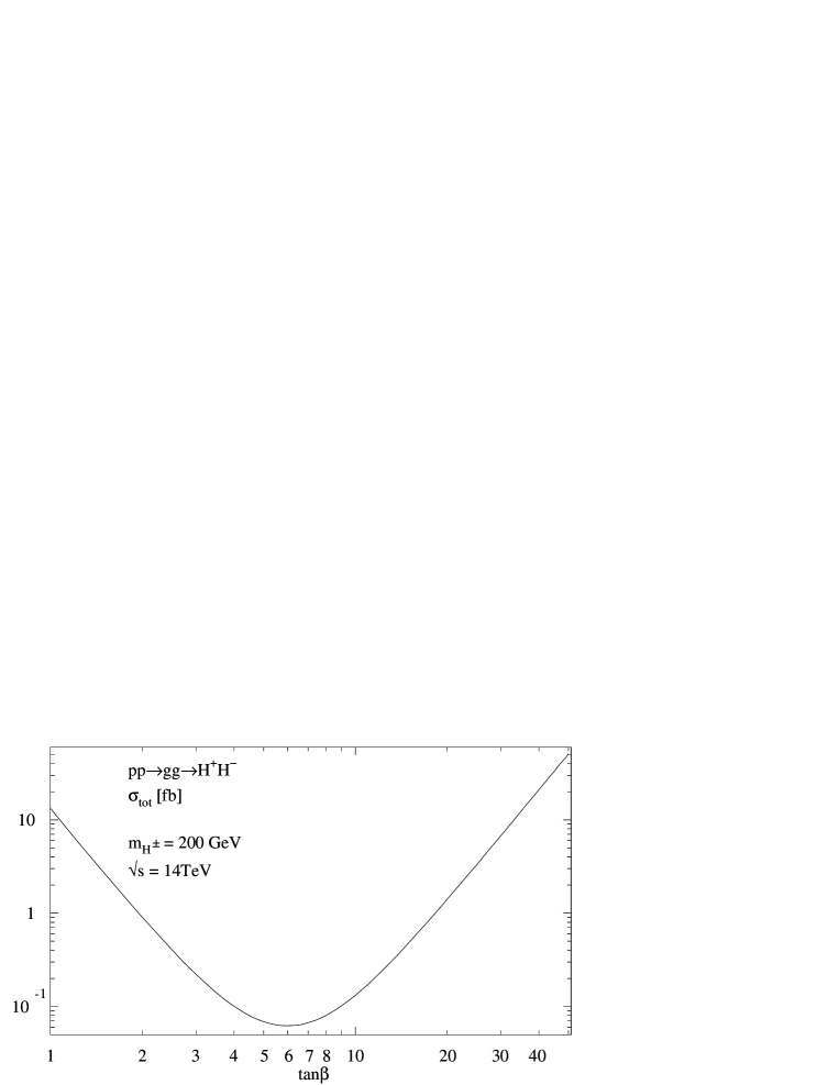
Figure 6: Dependence of the gluon-fusion cross section of charged Higgs-boson pairs on the parameter $\text{tan}\beta$.

We have evaluated the $pp$ cross section numerically for the LHC energy $\sqrt{s}=14\,$ TeV. The (pole) mass of the top quark has been set to $m_{t}=175$ GeV and the bottom quark mass to $m_{b}=5\,$GeV. The results are shown for three values $\text{tan}\beta=1.5,6$ and 30 in Fig. 5 as a function of the charged Higgs boson mass. [The masses of the neutral Higgs bosons $h^{0}$ and $H^{0}$ which enter through the charges $C^{Q}_{\triangle}$, are fixed by $m_{H^{\pm}}$ and $\text{tan}\beta$ in the MSSM.] For small values of $\text{tan}\beta$ and modest values of $m_{H^{\pm}}$, the triangle diagram provides the dominant contribution. With rising Higgs mass and for large $\text{tan}\beta$, the box diagrams become increasingly important; they dominate for Higgs masses above the top mass. The choice $\text{tan}\beta=6$ in Fig. 5 corresponds to the minimal value of the cross section. This is demonstrated in Fig. 6 for a fixed Higgs mass $m_{H^{\pm}}=200$ GeV and $\text{tan}\beta$ varied between 1 and 50. The minimal cross section is realized at $\text{tan}\beta\sim\sqrt{m_{t}/m_{b}}\sim 6$, roughly equivalent to the minimum of the average $QQH^{\pm}$ coupling $\langle g_{QQH^{\pm}}\rangle={\left(m_{t}^{2}\tan^{2}\!\beta+m_{b}^{2}\cot^{2}\!\beta\right)}^{1/2}$.

The cross section for gluon fusion of charged Higgs boson pairs is smaller than the cross section for the Drell–Yan mechanism. In the interesting mass range $m_{H^{\pm}}>200\,$ GeV, the ratio is about $0.4$ and $0.2$ for $\text{tan}\beta=30$ and $1.5$ respectively. It is noteworthy that the angular distributions of the charged Higgs bosons are different for the two mechanisms. While the Drell–Yan mechanism generates a $\sin^{2}\!\theta$ distribution in the $(H^{+}H^{-})$ center-of-mass frame, the gluon-fusion processes are not suppressed by angular-momentum conservation in the forward direction; for example, the amplitudes built up by the Higgs exchange diagrams, are isotropic in $\theta$. Even though the gluon-fusion mechanism is not dominant for the production of charged Higgs-boson pairs, it is nevertheless of great interest since the $gg$ fusion cross section and the angular distribution are affected by the size of the trilinear self-couplings between the CP-even neutral and charged Higgs bosons.

4 Conclusions

As shown in the representative examples of Fig. 5, the cross sections for charged Higgs masses below 300 GeV vary between 1 and 10 fb in a large part of the MSSM parameter space. This corresponds to rates of 100 and 1,000 events for an integrated luminosity of $\int{\cal L}=100\,\text{fb}^{-1}$, which is expected in a year of high-luminosity runs at the LHC. For small Higgs masses the triangle contribution appears large enough to generate a significant transition amplitude; this will enable us to measure the trilinear self-couplings $\lambda_{H^{+}H^{-}h^{0}}$ and $\lambda_{H^{+}H^{-}H^{0}}$ of the CP-even neutral and charged Higgs bosons. Charged Higgs particles decay predominantly to $\tau\nu_{\tau}$ final states at large $\text{tan}\beta$, leading to asymmetric $\tau^{+}\tau^{-}$ configurations in the decays of the two Higgs particles. For small $\text{tan}\beta$, the potentially dominant chargino/neutralino decays are more difficult to control experimentally. These experimental problems must be approached, however, in dedicated detector and background simulations, which are beyond the scope of this first-step theoretical analysis.

Acknowledgement:
We thank V.A. Smirnov for valuable discussions on the heavy-mass expansion of Feynman diagrams.

APPENDICES

1. Form factors in $gg\rightarrow H^{+}H^{-}$

Parameter definitions:

$$\hat{s} =(p_{a}+p_{b})^{2},\qquad\hat{t} =(p_{a}-p_{c})^{2},\qquad\hat{u} =(p_{b}-p_{c})^{2}\qquad\qquad\qquad\qquad$$

$$\hat{t}_{1} =\hat{t}-m_{H^{\pm}}^{2},\qquad\hat{u}_{1} =\hat{u}-m_{H^{\pm}}^{2},\qquad p_{t}^{2} =\hat{t_{1}}\hat{u_{1}}/{\hat{s}}-m_{H^{\pm}}^{2}$$

$$\tau_{Q} =4m_{Q}^{2}/\hat{s},\qquad\quad\hat{\beta} =\left(1-4m_{H^{\pm}}^{2}/\hat{s}\right)^{1/2}$$

Scalar integrals [16]:

$$C^{\alpha\beta\gamma}_{ij} =\int\frac{d^{4}q}{i\pi^{2}}\frac{1}{\left[q^{2}-m_{\alpha}^{2}\right]\left[{\left(q+p_{i}\right)}^{2}-m_{\beta}^{2}\right]\left[{\left(q+p_{i}+p_{j}\right)}^{2}-m_{\gamma}^{2}\right]}$$

$$D^{\alpha\beta\gamma\delta}_{ijk} =\int\frac{d^{4}q}{i\pi^{2}}\frac{1}{\left[q^{2}-m_{\alpha}^{2}\right]\left[{\left(q+p_{i}\right)}^{2}-m_{\beta}^{2}\right]\left[{\left(q+p_{i}+p_{j}\right)}^{2}-m_{\gamma}^{2}\right]\left[{\left(q+p_{i}+p_{j}+p_{k}\right)}^{2}-m_{\delta}^{2}\right]}$$

$$\phantom{sss}\text{with}\phantom{sss}\alpha,\beta,\gamma,\delta=t,b\,\quad\text{and}\quad i,j,k=1,\ldots,4$$

$$\phantom{ssswithsss}p_{1}=p_{a}\,,\;p_{2}=p_{b}\,,\;p_{3}=-p_{c}\,,\;p_{4}=-p_{d}\;\;\;\text{in}\;\;\;a+b\rightarrow c+d$$

Tensor basis:

$$P=+\qquad S_{z}=0\,:\quad A_{1}^{\mu\nu}=g^{\mu\nu}-\frac{p_{a}^{\nu}p_{b}^{\mu}}{\left(p_{a}p_{b}\right)}$$

$$S_{z}=2\,:\quad A_{2}^{\mu\nu}=g^{\mu\nu}+\frac{p_{c}^{2}p_{a}^{\nu}p_{b}^{\mu}}{p_{t}^{2}\left(p_{a}p_{b}\right)}-\frac{2\left(p_{b}p_{c}\right)p_{a}^{\nu}p_{c}^{\mu}}{p_{t}^{2}\left(p_{a}p_{b}\right)}-\frac{2\left(p_{a}p_{c}\right)p_{b}^{\mu}p_{c}^{\nu}}{p_{t}^{2}\left(p_{a}p_{b}\right)}+\frac{2p_{c}^{\mu}p_{c}^{\nu}}{p_{t}^{2}}$$

$$P=-\qquad S_{z}=0\,:\quad\bigg{[}A_{3}^{\mu\nu}=\frac{1}{\left(p_{a}p_{b}\right)}\epsilon^{\mu\nu p_{a}p_{b}}\;\text{: CP odd }\Rightarrow\text{ not coupling to }H^{+}H^{-}\,\bigg{]}$$

$$S_{z}=2\,:\quad A_{4}^{\mu\nu}=\frac{p_{c}^{\mu}\epsilon^{\nu p_{a}p_{b}p_{c}}+p_{c}^{\nu}\epsilon^{\mu p_{a}p_{b}p_{c}}+\left(p_{b}p_{c}\right)\epsilon^{\mu\nu p_{a}p_{c}}+\left(p_{a}p_{c}\right)\epsilon^{\mu\nu p_{b}p_{c}}}{\left(p_{a}p_{b}\right)p_{t}^{2}}$$

normalization and orthogonality: $A_{i}A_{j}=2\delta_{ij}$

Matrix element:

$${\cal M}\left(g_{a}g_{b}\rightarrow H^{+}H^{-}\right) ={\cal M}_{\triangle}+{\cal M}_{\Box}$$

$${\cal M}_{\triangle} =\frac{G_{F}\alpha_{s}\hat{s}}{2\sqrt{2}\pi}\sum_{Q=t,b}C_{\triangle}^{Q}F^{Q}_{\triangle}A_{1\mu\nu}\epsilon_{a}^{\mu}\epsilon_{b}^{\nu}\delta_{ab}$$

$${\cal M}_{\Box} =\frac{G_{F}\alpha_{s}\hat{s}}{2\sqrt{2}\pi}\left(F_{\Box}A_{1\mu\nu}+G_{\Box}A_{2\mu\nu}+H_{\Box}A_{4\mu\nu}\right)\epsilon_{a}^{\mu}\epsilon_{b}^{\nu}\delta_{ab}\qquad\qquad$$

Triangle form factor:

$$F^{Q}_{\triangle} =\tau_{Q}\left[1+\left(1-\tau_{Q}\right)f\left(\tau_{Q}\right)\right]$$

$$\phantom{=s}f\left(\tau_{Q}\right)=\left\{\begin{array}[]{rl}-\frac{1}{4}{\left[\text{log}\left(\frac{1+\sqrt{1-\tau_{Q}}}{1-\sqrt{1-\tau_{Q}}}\right)-i\pi\right]}^{2}&:\;\;\tau_{Q}\leq 1\\ &\\ {\text{arcsin}}^{2}\frac{1}{\sqrt{\tau_{Q}}}&:\;\;\tau_{Q}>1\end{array}\right.\qquad\qquad\qquad\quad$$

Box form factors:

$$F_{\Box}^{1}=\frac{2m_{b}^{2}}{\hat{s}} \bigg{[}\left(1+2m_{t}^{2}C_{12}^{ttt}\right)+\left(m_{t}^{2}+m_{b}^{2}-m_{H^{\pm}}^{2}\right)\Big{\{}-\frac{\hat{t}_{1}}{\hat{s}}C_{13}^{ttb}-\frac{\hat{u}_{1}}{\hat{s}}C_{23}^{ttb}+m_{t}^{2}\left(D_{123}^{tttb}+D_{213}^{tttb}\right)\qquad\qquad\qquad\qquad\qquad\qquad$$

$$+\frac{1}{2}\left(m_{t}^{2}+m_{b}^{2}+p_{t}^{2}\right)D_{132}^{ttbb}\Big{\}}\bigg{]}+\,\frac{2m_{b}^{2}}{\hat{s}}\bigg{[}b\leftrightarrow t\bigg{]}$$

$$F_{\Box}^{2}=F^{1}_{\Box}\left(m_{t}\leftrightarrow m_{b}\right)\qquad\qquad\qquad\qquad\qquad\qquad\qquad\qquad\qquad\qquad\quad\qquad\qquad\qquad\qquad\qquad\qquad$$

$$F_{\Box}^{3}=2m_{b}^{2}m_{t}^{2} \bigg{[}-\frac{4\hat{t}_{1}}{\hat{s}^{2}}C_{13}^{ttb}-\frac{4\hat{u}_{1}}{\hat{s}^{2}}C_{23}^{ttb}+\Big{(}\frac{4m_{t}^{2}}{\hat{s}}-1\Big{)}\left(D_{123}^{tttb}+D_{213}^{tttb}\right)+\Big{\{}\frac{2}{\hat{s}}\left(m_{t}^{2}+m_{b}^{2}+p_{t}^{2}\right)-1\Big{\}}D_{132}^{ttbb}\bigg{]}$$

$$+\,2m_{b}^{2}m_{t}^{2} \bigg{[}b\leftrightarrow t\bigg{]}\qquad\qquad\phantom{s}$$

$$G_{\Box}^{1}=\frac{m_{b}^{2}}{p_{t}^{2}}\bigg{[} \Big{\{}\frac{\hat{s}}{2}-p_{t}^{2}+M^{4}_{bt}\Big{\}}C_{12}^{bbb}+N(\hat{t}_{1})C_{13}^{ttb}+N(\hat{u}_{1})C_{23}^{ttb}+\Big{(}\frac{\hat{s}}{2}+m_{b}^{2}+m_{t}^{2}-m_{H^{\pm}}^{2}\Big{)}\Big{(}{\hat{\beta}}^{2}-\frac{2p_{t}^{2}}{\hat{s}}\Big{)}C_{34}^{tbt}\;$$

$$+ \Big{\{}M^{6}+L_{bt}(\hat{t}_{1},\hat{u}_{1})\Big{\}}D_{123}^{bbbt}+\Big{\{}M^{6}+L_{bt}(\hat{u}_{1},\hat{t}_{1})\Big{\}}D_{213}^{bbbt}+\Big{\{}M^{6}+\left(m_{b}^{4}+m_{t}^{4}\right)\Big{(}\frac{1}{2}+\frac{p_{t}^{2}-m_{H^{\pm}}^{2}}{\hat{s}}\Big{)}$$

$$+ \left(m_{b}^{2}+m_{t}^{2}\right)p_{t}^{2}\Big{(}\frac{1}{2}-\frac{m_{H^{\pm}}^{2}}{\hat{s}}\Big{)}\Big{\}}D_{132}^{ttbb}\bigg{]}+\,\frac{m_{b}^{2}}{p_{t}^{2}}\bigg{[}b\leftrightarrow t\bigg{]}$$

where: $$M^{4}_{bt}=\frac{2}{\hat{s}}\Big{[}{\big{(}m_{t}^{2}-m_{H^{\pm}}^{2}\big{)}}^{2}-m_{b}^{4}\Big{]}+2\left(m_{t}^{2}-m_{H^{\pm}}^{2}\right)$$

$$M^{6}=\frac{m_{t}^{6}-m_{t}^{4}m_{b}^{2}-m_{t}^{2}m_{b}^{4}+m_{b}^{6}}{\hat{s}}+m_{b}^{2}m_{t}^{2}\Big{(}2\frac{\hat{t}_{1}\hat{u}_{1}}{{\hat{s}}^{2}}-1\Big{)}$$

$$N(\hat{t}_{1})=\frac{\hat{t}_{1}}{\hat{s}}\Big{[}2\big{(}m_{H^{\pm}}^{2}-m_{b}^{2}-m_{t}^{2}\big{)}\frac{\hat{t}}{\hat{s}}+\frac{{\hat{t}_{1}}^{2}}{\hat{s}}\Big{]}$$

$$L_{bt}(\hat{t}_{1},\hat{u}_{1})=m_{b}^{4}\left[\frac{1}{2}+\frac{\hat{u}_{1}}{\hat{s}}\Big{(}1-\frac{\hat{u}_{1}}{\hat{s}}\Big{)}+\frac{p_{t}^{2}}{\hat{s}}\right]+m_{t}^{4}\left[\frac{1}{2}-\frac{2\hat{u}+m_{H^{\pm}}^{2}}{\hat{s}}\right]$$

$$\qquad\qquad\;\,+m_{b}^{2}\left[\frac{{\hat{\beta}}^{2}p_{t}^{2}}{2}-\frac{m_{H^{\pm}}^{4}}{\hat{s}}\right]+m_{t}^{2}\left[\frac{\hat{u}}{\hat{s}}\left(2\hat{u}+\hat{t}\right)-\frac{p_{t}^{2}}{2}\right]-\frac{\hat{u}}{\hat{s}}\left[\frac{{\hat{u}_{1}}^{2}}{2}+\hat{u}\,m_{H^{\pm}}^{2}\right]\qquad\qquad\qquad$$

$$G_{\Box}^{2}=G_{\Box}^{1}\left(m_{t}\leftrightarrow m_{b}\right)\qquad\qquad\qquad\qquad\qquad\qquad\qquad\qquad\qquad\qquad\qquad\qquad\qquad\qquad\qquad\qquad\qquad\,$$

$$G_{\Box}^{3}=\frac{4m_{t}^{2}m_{b}^{2}}{\hat{s}p_{t}^{2}} \bigg{[}-\left(2m_{t}^{2}-2m_{b}^{2}+2m_{H^{\pm}}^{2}-\hat{s}\right)C_{12}^{ttt}-\frac{2\hat{t}_{1}\hat{t}}{\hat{s}}\,C_{13}^{ttb}-\frac{2\hat{u}_{1}\hat{u}}{\hat{s}}\,C_{23}^{ttb}+\left(\hat{s}-4m_{H^{\pm}}^{2}-2p_{t}^{2}\right)\,C_{34}^{tbt}$$

$$\;+L_{bt}(\hat{u})D_{123}^{tttb}+L_{bt}(\hat{t})D_{213}^{tttb}+\Big{\{}{\left(m_{t}^{2}-m_{b}^{2}\right)}^{2}+\left(m_{t}^{2}+m_{b}^{2}\right)p_{t}^{2}\Big{\}}D_{132}^{ttbb}\bigg{]}+\,\frac{4m_{t}^{2}m_{b}^{2}}{\hat{s}p_{t}^{2}}\bigg{[}b\leftrightarrow t\bigg{]}\qquad\qquad\qquad\qquad\qquad\qquad\qquad\quad$$

$$\phantom{G_{\Box}^{1}=s}\text{where:}\quad L_{bt}(\hat{u}) ={\left(m_{t}^{2}-m_{b}^{2}\right)}^{2}+\hat{u}\left(\hat{u}-2m_{b}^{2}\right)-2m_{t}^{2}\hat{u}_{1}^{2}/\hat{s}\qquad\text{and}\quad\hat{u}\Rightarrow\hat{t}\qquad\qquad\qquad\qquad\qquad\quad$$

$$H_{\Box}^{1}=\frac{m_{b}^{2}}{p_{t}^{2}} \bigg{[}\left(\hat{t}_{1}-\hat{u}_{1}\right)M_{bt}^{2}\,C_{12}^{ttt}+\frac{\hat{t}_{1}^{2}}{\hat{s}^{2}}\left(t+m_{H^{\pm}}^{2}\right)\,C_{13}^{ttb}-\frac{\hat{u}_{1}^{2}}{\hat{s}^{2}}\left(u+m_{H^{\pm}}^{2}\right)\,C_{23}^{ttb}+\Big{(}\frac{\hat{u}_{1}-\hat{t}_{1}}{2}\Big{)}{\hat{\beta}}^{2}\,C_{34}^{btb}$$

$$\,+R_{bt}(\hat{t}_{1},\hat{u}_{1})D_{123}^{bbbt}-R_{bt}(\hat{u}_{1},\hat{t}_{1})D_{213}^{bbbt}+\Big{(}\frac{\hat{u}_{1}-\hat{t}_{1}}{2\hat{s}}\Big{)}\Big{\{}{\Big{(}m_{t}^{2}-m_{b}^{2}\Big{)}}^{2}+\left(m_{t}^{2}+m_{b}^{2}\right)p_{t}^{2}\Big{\}}D_{132}^{ttbb}\bigg{]}$$

$$+\frac{m_{b}^{2}}{p_{t}^{2}} \bigg{[}b\leftrightarrow t\bigg{]}$$

where: $$R_{bt}(\hat{t}_{1},\hat{u}_{1})=\frac{1}{2}\left(\hat{u}+m_{H^{\pm}}^{2}\right)\frac{\hat{u}\hat{u}_{1}}{\hat{s}}+\frac{1}{2}\left(\frac{\hat{u}_{1}-\hat{t}_{1}}{\hat{s}}\right){\left(m_{t}^{2}-m_{b}^{2}\right)}^{2}$$

$$\phantom{ssssssssss}+m_{b}^{2}\left[\frac{\hat{u}_{1}^{2}}{\hat{s}^{2}}\left(\hat{t}_{1}-\hat{u}_{1}\right)+\frac{p_{t}^{2}}{2}\right]+m_{t}^{2}\left[\frac{\hat{u}}{\hat{s}}\left(\hat{t}_{1}-\hat{u}_{1}\right)-\frac{p_{t}^{2}}{2}\right]\qquad$$

$$M^{2}_{bt}=\frac{m_{H^{\pm}}^{2}+m_{t}^{2}-m_{b}^{2}}{\hat{s}}-\frac{1}{2}\qquad\qquad\qquad\qquad\qquad\qquad\qquad\qquad\qquad\qquad\qquad\qquad\qquad$$

$$H_{\Box}^{2}=-\,\frac{m_{t}^{2}}{m_{b}^{2}}\,H_{\Box}^{1}\qquad\qquad\qquad\qquad\qquad\qquad\qquad\qquad\qquad\qquad\qquad\qquad\qquad\qquad\qquad\qquad\qquad\qquad$$

$$H_{\Box}^{3}=0\qquad\qquad\qquad\qquad\qquad\qquad\qquad\qquad\qquad\qquad\qquad\qquad\qquad\qquad\qquad\qquad\qquad\qquad\qquad\qquad$$

2. Pinching top propagators

Because of delicate cancellations, the limit $m_{t}\rightarrow\infty$ is not easy to calculate for the box diagrams involving one $t$ line and three $b$ lines, etc. We have performed this limit for the amplitudes first in the Feynman parametrization. The problem however can also be solved in a systematic way by adopting the scheme for the expansion in the heavy-quark mass, which has been discussed in Ref. [17]. This method is technically easier than the Feynman parameter method. The limit is performed by expanding the scalar integrals inside the form factors; the $m_{t}$ contributions arising from the Yukawa couplings are factored out.

The procedure [17] will be illustrated for a scalar three-point function including one top propagator:

$$C_{k_{1}k_{2}}^{bbt}=\int\!\frac{d^{n}\!q}{i\pi^{2}}\frac{1}{\big{[}q^{2}-m_{b}^{2}\big{]}\big{[}{\left(q+k_{1}\right)}^{2}-m_{b}^{2}\big{]}\big{[}{\left(q+k_{1}+k_{2}\right)}^{2}-m_{t}^{2}\big{]}}\;,$$

which must be expanded up to ${\cal O}((k_{i}k_{j})^{2}/m_{t}^{6})$. The integral is apparently ultraviolet and infrared finite; nevertheless, we will work in $n$ dimensions in order to properly define the divergences that occur at intermediate steps of the calculation. Since the Taylor expansion with respect to the heavy quark mass

$$\frac{1}{{\left(q+k_{1}+k_{2}\right)}^{2}-m_{t}^{2}}=\underbrace{-\frac{1}{m_{t}^{2}}-\frac{{\left(q+k_{1}+k_{2}\right)}^{2}}{m_{t}^{4}}}_{N_{\,UV}}+...$$

leads to ultraviolet divergences of the integral at $q\rightarrow\infty$, the expansion cannot be applied in this na$\ddot{{\text{\i}}}$ve form. However, after regularizing the divergences in $n$ dimensions, $N_{\,UV}$ can be used in the identity

$$\frac{1}{{\left(q+k_{1}+k_{2}\right)}^{2}-m_{t}^{2}}=N_{\,UV}+\underbrace{\Big{[}\frac{1}{{\left(q+k_{1}+k_{2}\right)}^{2}-m_{t}^{2}}-N_{\,UV}\Big{]}}_{R_{IR}}\;.$$

to define a kernel

$$R_{IR}=\frac{(q+k_{1}+k_{2})^{2}}{m_{t}^{4}\left[(q+k_{1}+k_{2})^{2}-m_{t}^{2}\right]}$$

which, together with the two bottom-quark propagators in $C$, can be expanded in the variables $(qk_{i})/(q^{2}-m_{t}^{2})$, $(k_{i}k_{j})/m_{t}^{2}$ and $m_{b}^{2}/m_{t}^{2}$. After performing the integral of the expansion in $n$ dimensions, the leading terms generate singularities which exactly cancel the singularities of the integral over $N_{\,UV}$. The finite pieces and the subsequent terms of the expansion lead to a well-behaved series in inverse powers of the heavy quark mass. The expansion for this particular example can finally be written:

$$C_{k_{1}k_{2}}^{bbt} =\frac{1}{m_{t}^{2}}\left[1+\log\left(\frac{m_{b}^{2}}{m_{t}^{2}}\right)-g(\kappa_{b})\right]$$

$$+\frac{1}{m_{t}^{4}}\left[m_{b}^{2}\left(1+2\log\left(\frac{m_{b}^{2}}{m_{t}^{2}}\right)-g(\kappa_{b})\right)+\left(k_{1}k_{2}+k_{2}^{2}\right)\left(\frac{5}{2}+\log\left(\frac{m_{b}^{2}}{m_{t}^{2}}\right)-g(\kappa_{b})\right)+\frac{k_{1}^{2}}{2}\right]$$

$$+{\cal O}\left(\frac{(k_{i}k_{j})^{2}}{m_{t}^{6}}\right)\;,$$

where $\kappa_{b}=4m_{b}^{2}/k_{1}^{2}$ and

$$g(\kappa_{b})=\left\{\begin{array}[]{rl}2-\sqrt{1-\kappa_{b}}\left[\log\left\{\frac{1+\sqrt{1-\kappa_{b}}}{1-\sqrt{1-\kappa_{b}}}\right\}-i\pi\right]&:\;\;\kappa_{b}\leq 1\\ &\\ 2-2\sqrt{\kappa_{b}-1}\arcsin\frac{1}{\sqrt{\kappa_{b}}}&:\;\;\kappa_{b}>1\end{array}\right.$$

The same procedure can be applied to the large quark mass limit of scalar three-point functions including two top propagators. The product of the two top propagators is first na$\ddot{{\text{\i}}}$vely Taylor expanded. The top part is then split into UV- and IR-divergent contributions as shown before. After the Taylor-expansion of the IR-divergent part, the calculation of the integrals leads to:

$$C_{k_{1}k_{2}}^{ttb}= -\frac{1}{m_{t}^{2}}-\frac{1}{m_{t}^{4}}\bigg{[}m_{b}^{2}\bigg{(}1+\log\big{(}\frac{m_{b}^{2}}{m_{t}^{2}}\big{)}\bigg{)}\frac{k_{1}^{2}}{3}+\frac{k_{2}^{2}}{2}+\frac{k_{1}k_{2}}{2}\bigg{]}\qquad\qquad\qquad\qquad$$

$$+{\cal O}\Big{(}\frac{(k_{i}k_{j})^{2}}{m_{t}^{6}}\Big{)}\;.$$

For the scalar three-point function involving three top propagators, the na$\ddot{{\text{\i}}}$ve expansion is UV-finite, so that it need not be split. One obtains the following expansion up to the required order ${\cal O}((k_{i}k_{j})^{3}/m_{t}^{8})$:

$$C_{k_{1}k_{2}}^{ttt}= -\frac{1}{2}\frac{1}{m_{t}^{2}}-\frac{1}{m_{t}^{4}}\Big{[}\frac{k_{1}k_{1}+k_{1}k_{2}+k_{2}k_{2}}{12}\Big{]}$$

$$-\frac{1}{m_{t}^{6}}\Big{[}\frac{(k_{1}^{2}+k_{2}^{2})k_{1}k_{2}}{30}+\frac{k_{1}^{2}k_{2}^{2}}{36}+\frac{(k_{1}k_{2})^{2}}{45}+\frac{k_{1}^{4}+k_{2}^{4}}{60}\Big{]}\qquad\qquad\qquad\quad$$

$$+{\cal O}\Big{(}\frac{(k_{i}k_{j})^{3}}{m_{t}^{8}}\Big{)}\;.$$

The expansion of the four-point functions can be carried out in an analogous way. The result is still too long to be presented in plain text; yet the analytic expressions are available from [14].

In contrast to the expansion for large $t$ mass, the subsequent expansion for small $b$ mass $m_{b}^{2}/\hat{s}\ll 1$ is straightforward.

References

- [1] P. Fayet, Nucl. Phys. B90 (1975) 104; S. Dimopoulos and H. Georgi, Nucl. Phys. B193 (1981) 150; N. Sakai, Z. Phys. 11 (1981) 153; K. Inoue, A. Komatsu and S. Takeshita, Prog. Theor. Phys. 67 (1982) 927; E. Witten, Nucl. Phys. B231 (1984) 419; H. P. Nilles, Phys. Rep. 110 (1984) 1; H.E. Haber and G.L. Kane, Phys. Rep. 117 (1985) 75.
- [2] V. Barger, M.S. Berger and P. Ohmann, Phys. Rev. D49 (1994) 4908; A. Djouadi, et al., Z. Phys. C74 (1997) 93.
- [3] E. Richter-Was, D. Froidevaux, F. Gianotti, L. Poggioli, D. Cavalli and S. Resconi, Report CERN-TH/96-111.
- [4] J. Gunion, H.E. Haber, F. Paige, Wu-ki Tung and S.S.D. Willenbrock, Nucl. Phys. B294 (1987) 621; S. Moretti and K. Odagiri, Phys. Rev. D55 (1997) 5627.
- [5] E. Eichten, I. Hinchliffe, K. Lane and C. Quigg, Rev. Mod. Phys. 56 (1984) 579.
- [6] T. Plehn, M. Spira and P.M. Zerwas, Nucl. Phys. B479 (1996) 46.
- [7] S.S.D. Willenbrock, Phys. Rev. D35 (1987) 173.
- [8] J. Yi, H. Liang, M. Wen–Gan, Y. Zeng–Hui and H. Meng, J. Phys. G23 (1997) 385.
- [9] A. Djouadi, H.E. Haber and P.M. Zerwas, Phys. Lett. B375 (1996) 203.
- [10] J. Gunion and A. Turski, Phys. Rev. D39 (1989) 2701 and D40 (1990) 2333; M. Berger, Phys. Rev. D41 (1990) 225; Y. Okada, M. Yamaguchi and T. Yanagida, Prog. Theor. Phys. 85 (1991) 1; H. Haber and R. Hempfling, Phys. Rev. Lett. 66 (1991) 1815; J. Ellis, G. Ridolfi and F. Zwirner, Phys. Lett. B257 (1991) 83; R. Barbieri, F. Caravaglios and M. Frigeni, Phys. Lett. B258 (1991) 167; A. Yamada, Phys. Lett. B263 (1991) 233; A. Brignole, J. Ellis, G. Ridolfi and F. Zwirner, Phys. Lett. B271 (1991) 123; P.H. Chankowski, S. Pokorski and J. Rosiek, Phys. Lett. B274 (1992) 191; M. Drees and M.M. Nojiri, Phys. Rev. D45 (1992) 2482.
- [11] A. Brignole and F. Zwirner, Phys. Lett. B299 (1993) 72; H.E. Haber, in Perspectives on Higgs Physics, ed. G.L. Kane (World Scientific, Singapore, 1993).
- [12] M. Carena, J. Espinosa, M. Quiros and C.E.M. Wagner, Phys. Lett. B355 (1995) 209.
- [13] M. Spira, Report CERN-TH/97-68 (hep-ph/9705337).
- [14] A. Krause, Diploma Thesis, Univ. of Hamburg 1997; file: spira@@cern.ch.
- [15] H.L. Lai, et al., Phys. Rev. D55 (1997) 1280.
- [16] G. ’t Hooft and M. Veltman, Nucl. Phys. B153 (1979) 365.
- [17] For a recent review see V.A. Smirnov, Mod. Phys. Lett. A10 (1995) 1485.