HD-THEP-97-34 Diffractive color-dipole nucleon scattering

Abstract

We determine the diffractive scattering amplitude of a color-dipole on a nucleon using a non-perturbative model of QCD which contains only parameters taken from low-energy physics. This allows to relate specific features of the confinement mechanisms with diffractive electro-production processes and structure functions. The agreement with phenomenological data is satisfactory.

Introduction

In strong interaction physics the infra-red behavior of QCD is relevant both in the low- and high-energy domain. In hadron spectroscopy this is evident, but also in high-energy reactions at small momentum transfer non-perturbative effects play a crucial role. Normally the non-perturbative input in low-energy physics (e.g. intra-quark potentials) and high-energy physics (e.g. structure functions) are conceptually and computationally seen quite separately. In this letter we calculate the high-energy diffractive scattering of color-dipoles on a nucleon in a non-perturbative model of QCD, the parameters of which are fixed only by low-energy input. Our results are compared with other approaches and experimental data.

Since several years one of the authors (H.G.D.) and Yu.A. Simonov have proposed a model in which the non-perturbative features of QCD are approximated by a Gaussian stochastic process which is characterized by the gauge-invariant non-local gluon field-strength correlator [1]-[3]. This correlator is characterized by a correlation length $a$ and its value at zero separation, the gluon condensate $<g^{2}FF>$. This model of the stochastic vacuum (MSV) yields linear confinement [1] in a very simple and natural way; a nice feature of the model is that confinement only occurs in non-Abelian theories.

The MSV has also been applied to diffractive high-energy scattering [4]-[6], lepto-production of vector-mesons [7] and $\gamma^{*}p$-interaction [8]. Here the natural ingredient (see next section for more details) is the expectation value of two Wegner-Wilson-loops with light-like sides, which correspond to the world-lines of two color-neutral dipoles [9] [10][4]. A characteristic feature of the application of the MSV to diffractive high-energy scattering is the fact that the same mechanism, which is responsible for confinement, leads to a typical dependence of the cross-sections on the loop extensions (dipole sizes): Even if the dipole size is large as compared to the correlation length $a$ of the correlator, the total cross-section still increases with the dipole size. Thus the model implies string-string-interaction and can not lead to quark-additivity. Nevertheless, the ratio of the total cross-sections off nucleon-nucleon- and nucleon-meson-scattering agrees with experiment without additional parameters, this is due to the different radii of the nucleon and mesons, given by the electro-magnetic form-factor [4]. This dependence on the radii also leads to a typical relation between the total cross-section and the logarithmic slope of the elastic cross-section for different hadrons which is in agreement with the experimental data [4].

In this letter we concentrate on the high-energy diffractive scattering of a color-dipole of arbitrary size on a proton. This process is phenomenologically very interesting because it can be used to describe for example the diffractive electro-production of vector-mesons, where due to the photon wave-function (in light-cone perturbation theory [11][12]) dipoles of arbitrary size occur in the interaction. For the proton we use a diquark-picture, which works in all our applications to high-energy scattering better than a three-body-picture. Especially the necessary suppression of the coupling of the odderon to the nucleon is achieved in that way [5][6]. So, the electro-production of vector-mesons can be build from dipole-dipole-scattering and is illustrated in fig.(1).

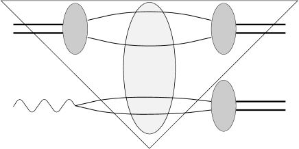
Figure 1: Diffractive electro-production of vector-mesons can be viewed as the diffractive scattering of color-dipoles ($q$-$\bar{q}$-pair for the photon and $q$-diquark-pair for the proton) folded with wave-functions. In this letter we calculate only the part inside the triangular, that is the diffractive scattering of the proton on a dipole of arbitrary size.

For large $Q^{2}$ the virtual photon (at least the longitudinal polarized one) interacts like a small dipole. In the phenomenological interesting regime dipole sizes between 0.1 fm and 1 fm are most interesting, where the cross-over from perturbative to non-perturbative physics occurs.
Dipole-proton-scattering amplitude

Nachtmann has developed a scheme which allows the separation of the hard high-energy scale from the soft scale of momentum transfer [9]. He considered quark-(anti-)quark-scattering first in an external gluon field in the eikonal approximation. In this way each (anti-)quark picks up the eikonal phase

$$\mbox{$\cal P$}e^{-ig\int_{C}\mbox{\bf A}_{\mu}(x){\rm d}x^{\mu}}$$ (1)

where the path $C$ is the classical (nearly) light-like path of the (anti-)quark, $\mbox{\bf A}_{\mu}$ is the matrix-valued color-potential and $\cal P$ stands for path ordering. The quantum transition amplitudes are obtained by functional integration over the color-field with the QCD-action as exponential weight. In our treatment of high-energy scattering we want to apply the MSV for this integration. We therefor consider not quark-quark-scattering but rather scattering of color-neutral dipoles. In that way we obtain from the eikonal factors (eq.(1)) Wegner-Wilson-loops, i.e. traces of line integrals around closed loops whose light-like sides are the paths of the constituents of the dipole (see fig.(2)). The scattering amplitude of two dipoles with transversal extension $\vec{R}_{1}$ and $\vec{R}_{2}$ respectively and impact parameter $\vec{b}$ is given by:

$$\tilde{J}(\vec{b},\vec{R}_{1},\vec{R}_{2})=-<\frac{1}{N_{C}}\makebox{ Tr }\left[\mbox{\bf W}[\partial S_{1}]-{\bf 1}\right]\cdot\frac{1}{N_{C}}\makebox{ Tr }\left[\mbox{\bf W}[\partial S_{2}]-{\bf 1}\right]>.$$ (2)

Figure 2: The two W-loops with transversal extension $\vec{R}_{1}$ and $\vec{R}_{2}$ and light-like sides. Loop 1 describes a color-dipole moving in negative $x^{3}$-direction and loop 2 a color-dipole moving in positive $x^{3}$-direction. The impact parameter $\vec{b}$ is chosen to be purely transversal.

The brackets ($<\dots>$) denote the functional integration over the gluon-field. In order to perform this integration we first transform the line integrals over $\mbox{\bf A}_{\mu}$ along the loops $\partial S_{1},\,\partial S_{2}$ in surface integrals over the field-strengths and then expand the exponentials. For the resulting functional integration over the field-strengths we use the ansatz of the MSV [1] [4]:

$$<g^{2}\,F_{\mu\nu}^{A}(z,w)\,F_{\rho\sigma}^{B}(0,w)>$$ (3)

$$= \frac{\delta^{AB}}{N_{C}^{2}-1}\frac{<g^{2}FF>}{12}\Big{\{}\kappa\left(g_{\mu\rho}g_{\nu\sigma}-g_{\mu\sigma}g_{\nu\rho}\right)D(z)$$

$$+(1-\kappa)\frac{1}{2}\left[\partial_{\mu}\left(z_{\rho}g_{\nu\sigma}-z_{\sigma}g_{\nu\rho}\right)+\partial_{\nu}\left(z_{\sigma}g_{\mu\rho}-z_{\rho}g_{\mu\sigma}\right)\right]D_{1}(z)\Big{\}}.$$

The correlation functions $D$ and $D_{1}$ are fitted to lattice results of the non-local correlator [13][14], they fall off on a length scale given by the correlation length $a$.
In leading order of the expansion of the W-loops we obtain a real scattering amplitude where only transversal coordinates enter. In ref. [4] only the $D$-function of the non-local correlator was taken into account. Including the $D_{1}$-function we find for eq.(2):

$$\tilde{J} = \frac{1}{8N_{C}^{2}(N_{C}^{2}-1)144}\tilde{\chi}^{2}$$

$$\tilde{\chi} = <g^{2}FF>\left(\kappa\,\int_{0}^{1}{\rm d}w_{1}\,\int_{0}^{1}{\rm d}w_{2}\,\left[\vec{r}_{1q}\cdot\vec{r}_{2q}\,\mbox{$\cal F$}_{2}[i\tilde{D}]\left(w_{1}\vec{r}_{1q}-w_{2}\vec{r}_{2q}\right)\right.\right.$$ (4)

$$\hskip 145.10922pt+\vec{r}_{1\bar{q}}\cdot\vec{r}_{2\bar{q}}\,\mbox{$\cal F$}_{2}[i\tilde{D}]\left(w_{1}\vec{r}_{1\bar{q}}-w_{2}\vec{r}_{2\bar{q}}\right)$$

$$\hskip 145.10922pt-\vec{r}_{1q}\cdot\vec{r}_{2\bar{q}}\,\mbox{$\cal F$}_{2}[i\tilde{D}]\left(w_{1}\vec{r}_{1q}-w_{2}\vec{r}_{2\bar{q}}\right)$$

$$\left.\hskip 145.10922pt-\vec{r}_{1\bar{q}}\cdot\vec{r}_{2q}\,\mbox{$\cal F$}_{2}[i\tilde{D}]\left(w_{1}\vec{r}_{1\bar{q}}-w_{2}\vec{r}_{2q}\right)\right]$$

$$\hskip 28.45274pt+(1-\kappa)\left[\mbox{$\cal F$}_{2}[i\tilde{D}_{1}^{\prime}]\left(\vec{r}_{1q}-\vec{r}_{2q}\right)\right.+\mbox{$\cal F$}_{2}[i\tilde{D}_{1}^{\prime}]\left(\vec{r}_{1\bar{q}}-\vec{r}_{2\bar{q}}\right)$$

$$\hskip 68.28644pt-\mbox{$\cal F$}_{2}[i\tilde{D}_{1}^{\prime}]\left(\vec{r}_{1q}-\vec{r}_{2\bar{q}}\right)-\left.\mbox{$\cal F$}_{2}[i\tilde{D}_{1}^{\prime}]\left(\vec{r}_{1\bar{q}}-\vec{r}_{2q}\right)\right]\bigg{)}.$$

The vectors $\vec{r}$ are defined in fig.(3) and $\mbox{$\cal F$}_{2}$ denotes the two dimensional Fourier-transformed of the correlation functions $D$ and $D_{1}$ in the transversal plane. Using the explicit ansatz given in ref. [4] we have:

$$\mbox{$\cal F$}_{2}[i\tilde{D}(\vec{k})](\vec{x}) = \int\,\frac{{\rm d^{2}}k}{(2\pi)^{2}}i\tilde{D}(\vec{k})e^{i\vec{k}\cdot\vec{x}}$$

$$= \frac{\pi}{2}\left[6\frac{|\vec{x}|^{2}}{\lambda^{2}}K_{2}\left(\frac{|\vec{x}|}{\lambda}\right)-\frac{|\vec{x}|^{3}}{\lambda^{3}}K_{3}\left(\frac{|\vec{x}|}{\lambda}\right)\right]\lambda^{2}$$

$$\mbox{$\cal F$}_{2}[i\tilde{D}_{1}^{\prime}(\vec{k})](\vec{x}) = \pi\frac{|\vec{x}|^{3}}{\lambda^{3}}K_{3}\left(\frac{|\vec{x}|}{\lambda}\right)\lambda^{4}$$

$$\lambda = \frac{8}{3\pi}a.$$ (5)

Here $K_{\nu}$ denotes the modified Bessel-functions of second order. One of the $w$-integrations in eq.(4) can be performed analytically [4].

Figure 3: Dipole-dipole-scattering in the transversal plane: $\vec{R}_{i}$ points from the quark of dipole $i$ to the anti-quark; $\vec{b}$ is the impact parameter and $\vec{r}_{iq(\bar{q})}$ points from the origin to the (anti-)quark of dipole $i$.

We also include the perturbative interaction which dominates the short distance behavior of the correlation function $D_{1}$. We use the perturbative expression for the non-local correlator in first order with a infra-red cutoff in agreement with the lattice results [14]:

$$<g^{2}\,F_{\mu\nu}^{A}(z)\,F_{\rho\sigma}^{B}(0)>_{\rm per}$$

$$= \delta^{AB}g^{2}\int\,\frac{{\rm d^{4}}k}{(2\pi)^{4}}\;e^{-ikz}\left(-g_{\nu\sigma}k_{\mu}k_{\rho}+g_{\nu\rho}k_{\mu}k_{\sigma}-g_{\mu\rho}k_{\nu}k_{\sigma}+g_{\mu\sigma}k_{\nu}k_{\rho}\right)\tilde{D}_{\rm per}^{\prime}(k)$$

with

$$\tilde{D}_{\rm per}^{\prime}(k)=\frac{i}{k^{2}-\frac{1}{c^{2}}},\;c=0.45\makebox{ fm}.$$

For the coupling constant we use here a frozen value of $\alpha_{s}\approx 0.5$, which is prescribed by our model for consistency reasons [15]-[17]. The perturbative contribution results in an additional term to $\tilde{\chi}$ (eq.(4)):

$$\tilde{\chi}_{\rm per} = -\frac{12i}{4}\int_{S_{1}}\int_{S_{2}}<g^{2}\,F_{\mu\nu}^{A}(x,w)\,F_{\rho\sigma}^{A}(y,w)>_{\rm per}\,{\rm d}\sigma^{\mu\nu}(x)\,{\rm d}\sigma^{\rho\sigma}(y)$$ (7)

$$= 12(N_{C}^{2}-1)g^{2}\left[\Delta\left(\vec{r}_{1q}-\vec{r}_{2q}\right)\right.+\Delta\left(\vec{r}_{1\bar{q}}-\vec{r}_{2\bar{q}}\right)-$$

$$\hskip 76.82234pt\Delta\left(\vec{r}_{1q}-\vec{r}_{2\bar{q}}\right)-\left.\Delta\left(\vec{r}_{1\bar{q}}-\vec{r}_{2q}\right)\right]$$

with

$$\Delta(\vec{x})=\mbox{$\cal F$}_{2}\left[\frac{1}{\vec{k}^{2}+\frac{1}{c^{2}}}\right](\vec{x})=\frac{1}{2\pi}K_{0}\left[\frac{|\vec{x}|}{c}\right].$$ (8)

Because the function $\tilde{\chi}$ enters quadratically in the scattering amplitude (see eq.(4)) we have in addition to the purely perturbative and non-perturbative contribution also an interference term.
In order to come from dipole-dipole- to dipole-hadron-scattering we smear the scattering amplitude (eq.(2)) with a transversal proton wave-function with extension parameter $S_{p}$ and keep one extension fixed to the dipole size $R_{\rm D}$:

$$\hat{J}(\vec{b},R_{\rm D},S_{p})=\int\,\frac{{\rm d}\varphi_{\rm D}}{2\pi}\int\,{\rm d^{2}}R_{2}\,\tilde{J}(\vec{b},\vec{R}_{\rm D},\vec{R}_{2})|\Psi(\vec{R}_{2},S_{p})|^{2}.$$ (9)

The scattering amplitude at center of mass energy $s$ and momentum transfer $t=-\vec{q}\,^{2}$ is given by:

$$T(s,t)=2is\int\,{\rm d^{2}}b\,e^{-i\vec{q}\,\vec{b}}\,\hat{J}(\vec{b},R_{\rm D},S_{p}).$$ (10)

For the proton (working in the diquark-picture [5] [6]) we use as wave-function:

$$|\Psi(\vec{R}_{2},S_{p})|^{2}=\frac{1}{2\pi}\frac{1}{S_{p}^{2}}e^{-\frac{|\vec{R}_{2}|^{2}}{2S_{p}^{2}}}.$$ (11)

For the total cross-section follows:

$$\sigma^{\rm tot}=\frac{1}{s}{\rm Im}T(s,0)=2\int\,{\rm d^{2}}b\,{\rm Re}[\hat{J}(\vec{b},R_{\rm D},S_{p})],$$ (12)

which in our model is independent of the center of mass energy $s$.

Numerical results and comparison with other approaches and experimental data

Nikolaev and Zakharov developed a picture of dipole-nucleon scattering [18]- [21] which is in some respect very similar to the one discussed above. But whereas our main emphasis lies on the calculation of the scattering amplitude $\hat{J}(\vec{b},R_{\rm D},S_{p})$ (eq.(9)) they are more interested in the consequences of the dipole-scattering picture especially in the energy dependence due to perturbative QCD. In a recent analysis Nemchik et al. extracted from electro-production data the dipole-proton cross-section $\sigma^{\rm tot}(s,R_{{\rm D}1})$ [22][23]. They used the fact that due to the overlap of the wave-functions of the photon with virtuality $Q^{2}$ and the produced vector-meson of mass $M_{V}$ the dipole-nucleon cross-section is manly probed at the so called scanning radius [24]

$$r_{s}\approx\frac{6}{\sqrt{Q^{2}+M_{V}^{2}}}.$$

The results of there analysis of different experiments are shown in fig.(4). There are two distinct domains of energy of the $\gamma^{*}-p$-system: The fixed target experiments of the EMC, NMC, E687 and FNAL groups are at the center of mass energy about $W\approx 10-15$ GeV, whereas the HERA experiments are at $W\approx 70-150$ GeV. The high-energy results are indeed systematically higher than the fixed target results but here we do not discuss this point which is off course of great interest for itself.

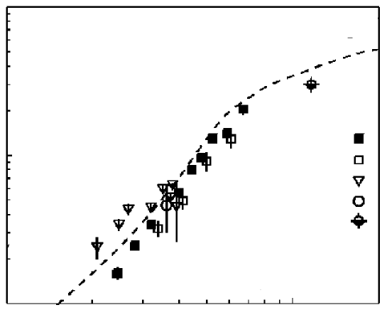
Figure 4: Comparison of our result for the total cross-section for dipole (extension $R_{{\rm D}1}$) proton scattering with values extracted from cross-sections of lepto-production of vector-mesons by the method of Nemchik et al. [22][23]. The solid line is our result without any fitting of the parameters to high-energy data. The dashed line is the ansatz of Nemchik et al. for the total cross-section for the fixed target experiments.

The solid line in fig.(4) is our prediction for the dipole-proton cross-section where only low-energy input has been used: the correlator (eq.(3)) taken from the lattice calculations (compatible with the string tension of heavy quarkonia) and the electro-magnetic proton radius ($R^{\rm em}=0.862$ fm [25]). We see that the agreement with the extracted phenomenological points is satisfactory and encourages the approach to relate high- and low-energy data.
Of special interest is the agreement of our calculation at values of $R_{{\rm D}1}$ larger than the correlation length $a\approx 0.3$ fm. If quark-additivity would hold the dipole cross-section should level off around that value of $R_{{\rm D}1}$. The continued increase shows that the most specific feature of non-perturbative QCD, namely confinement, leaves its traces also in high-energy scattering.

Acknowledgments

The authors want to thank A. Hebecker, O. Nachtmann and H.J. Pirner for discussions. M.R. thanks the Deutsche Forschungsgemeinschaft for financial support.

References

- [1] H.G. Dosch, Phys.Lett. B190 (1987) 177.
- [2] H.G. Dosch and Y.A. Simonov, Phys.Lett. B205 (1988) 339.
- [3] Y.A. Simonov, Nucl.Phys. B307 (1988) 512.
- [4] H.G. Dosch, E. Ferreira and A. Krämer, Phys.Rev. D50 (1994) 1992.
- [5] M. Rueter and H.G. Dosch, Phys.Lett. B380 (1996) 177.
-
[6]
M. Rueter, Proceedings of the workshop “Diquarks III”, Torino,
hep-ph-9612338 (1996). -
[7]
H.G. Dosch, T. Gousset, G. Kulzinger and H.J. Pirner,
Phys.Rev. D55 (1997) 2602. - [8] H.G. Dosch, T. Gousset and H.J. Pirner, hep-ph-9707264 (1997).
- [9] O. Nachtmann, Annals Phys. 209 (1991) 436.
- [10] O. Nachtmann, Lectures, Schladming (Austria), hep-ph-9609365 (1996).
- [11] J.D. Bjorken, J.B. Kogut and D.E. Soper, Phys.Rev. D3 (1971) 1382.
- [12] G.P. Lepage and S.J. Brodsky, Phys.Rev. D22 (1980) 2157.
- [13] A. Di Giacomo and H. Panagopoulos, Phys.Lett. B285 (1992) 133.
-
[14]
A. Di Giacomo, E. Meggiolaro and H. Panagopoulos,
hep-lat-9603017 (1996). - [15] M. Rueter and H.G. Dosch, Z.Phys. C66 (1995) 245.
- [16] H.G. Dosch, O. Nachtmann and M. Rueter, hep-ph-9503386 (1995).
- [17] M. Rueter, Proceedings of the conference “Quark Confinement and the Hadron Spectrum II”, Como, hep-ph-9610215 (1996).
- [18] N.N. Nikolaev and B.G. Zakharov, Z.Phys. C49 (1991) 607.
- [19] N.N. Nikolaev and B.G. Zakharov, Z.Phys. C53 (1992) 331.
- [20] N.N. Nikolaev and B.G. Zakharov, Z.Phys. C64 (1994) 631.
- [21] N.N. Nikolaev and B.G. Zakharov, Phys.Lett. B327 (1994) 149.
-
[22]
J. Nemchik, N.N. Nikolaev, E. Predazzi and B.G. Zakharov,
Phys.Lett. B374 (1996) 199. -
[23]
J. Nemchik, N.N. Nikolaev, E. Predazzi and B.G. Zakharov,
hep-ph-9605231 (1996). -
[24]
J. Nemchik, N.N. Nikolaev and B.G. Zakharov,
Phys.Lett. B341 (1994) 228. - [25] G.G. Simon et al., Z. Naturforsch. A35 (1980) 1.