3D EFFECTIVE THEORIES FOR THE
STANDARD MODEL AND EXTENSIONS

The construction and analysis of 3d effective theories for the description of the thermodynamics of the cosmological electroweak phase transition are reviewed. For the Standard Model and for the MSSM with stops somewhat heavier than the top, the effective theory is 3d SU(2)+Higgs, and the transition is strong enough for baryogenesis at no Higgs mass for the Standard Model, and up to $m_{H}\mathop{\raise 1.03334pt\hbox{$<$\kern-6.0pt\raise-3.7889pt\hbox{$\sim$}}}80$ GeV for the MSSM. For lighter stops, the effective theory is SU(3)$\times$SU(2) + two scalars and the transition could be strong enough up to $m_{H}\sim 100$ GeV. However, a lattice study in 3d is needed to confirm the last bound.

1 Introduction

The cosmological electroweak phase transition offers the prospect of connecting perturbative physics measurable at accelerator experiments, such as the Higgs mass, to non-perturbative astrophysical consequences, such as the matter-antimatter asymmetry and the galactic magnetic fields. Progress in recent years (for a review, see $\!{}^{{\bf?}}$) has made at least parts of this connection quantitative. The purpose of this talk is to review the part which is perhaps best under control: the equilibrium thermodynamics of the electroweak phase transition.

More specifically, the physics questions under consideration are: given the zero temperature vacuum Lagrangian and the corresponding parameters (the Higgs mass $m_{H}$, etc),

• is there a phase transition at some critical temperature $T_{c}$? If there is one, what is the order of that transition?

• if the transition is of the first order, what are the latent heat, the surface tension, and the discontinuity in the expectation value of the Higgs field characterizing the transition?

• what are the correlation lengths of different excitations around $T_{c}$?

Of course, the answers to these questions are just the first step in the study of the physical consequences of the transition. The equilibrium real time processes — such as the sphaleron rate and the plasmon properties — not to mention the whole class of non-equilibrium processes — such as bubble growth, rates of different processes in the bubble wall background, CP-violation, etc — remain outside of the present discussion. It is certainly only these phenomena which constitute the real physics possibly responsible, e.g., for baryon number or magnetic field generation. However, knowing the equilibrium thermodynamics is a necessary starting point: it gives the “ground state” around which non-equilibrium phenomena take place.

In fact, there is also one important quantitative constraint given (to a large extent) by thermodynamical considerations. This follows from the fact that if a baryon asymmetry has been generated at the electroweak phase transition, it must be preserved afterwards until present day. As non-thermodynamical input into this constraint go the sphaleron rate in the broken phase $\!{}^{{\bf?},{\bf?},{\bf?}}$, and the expansion rate of the Universe (which is however determined by the equation of state). The thermodynamical constraint to be satisfied can then be expressed as $\!{}^{{\bf?},{\bf?}}$

$$\frac{v(T_{c})}{T_{c}}\mathop{\raise 1.29167pt\hbox{$>$\kern-7.5pt\raise-4.73611pt\hbox{$\sim$}}}1.0\ldots 1.5,$$ (1)

where $v(T_{c})$ is the expectation value of the Higgs field in the broken phase in, say, the Landau gauge.

Unfortunately, even solving for the equilibrium thermodynamics of the electroweak phase transition is quite a difficult task, even though the theory is weakly coupled. This is due to the infrared (IR) problem at finite temperature $\!{}^{{\bf?},{\bf?}}$. Indeed, the perturbative expansion parameters of a finite temperature system differ from those of the same system at zero temperature. If the vacuum theory has the coupling $g^{2}$, then at finite temperature some loops are, instead, proportional to

$$g^{2}n_{b}(E)=\frac{g^{2}}{e^{E/T}-1}\stackrel{{\scriptstyle E\ll T}}{{\sim}}\frac{g^{2}T}{E}.$$ (2)

Here $n_{b}(E)$ is the Bose distribution function and $E$ is the typical energy or mass scale of the particles contributing. For example, in the effective potential $V(\phi)$ for the Higgs field $\phi$ appear terms of the type

$$\begin{array}[]{ccccc}\frac{T}{4\pi}g^{3}\phi^{3}&\frac{T^{2}}{(4\pi)^{2}}g^{4}\phi^{2}&\frac{T^{3}}{(4\pi)^{3}}g^{5}\phi&\frac{T^{4}}{(4\pi)^{4}}g^{6}&\ldots\\ &&&&\\ ({\rm\scriptstyle 1-loop})&({\rm\scriptstyle 2-loop})&({\rm\scriptstyle 3-loop})&({\rm\scriptstyle 4-loop})&\end{array}$$ (3)

For the Standard Model, the numerical coefficients in the 1-loop and 2-loop $\!{}^{{\bf?}}$ terms have been computed explicitly, and that of the 3-loop term has been determined on the lattice $\!{}^{{\bf?}}$. It follows that the expansion parameter is

$$\epsilon\sim\frac{g^{2}T}{\pi m_{W}},$$ (4)

where $m_{W}\sim{\frac{1}{2}}{g\phi}$. In perturbation theory the transition is between $\phi=0$ and $\phi\sim gT$; hence $\epsilon$ is not small and the perturbative description might, a priori, be quite unreliable. This estimate may get modified in extensions of the Standard Model $\!{}^{{\bf?}}$, but especially the symmetric phase always remains non-perturbative.

It is hence clear that to solve for the equilibrium thermodynamics of the electroweak phase transition, one needs a non-perturbative method. In principle the most straightforward is to put the 4d theory on the lattice and to make 4d lattice simulations $\!{}^{{\bf?}}$${}^{-\,}$$\!{}^{{\bf?}}$. Unfortunately, this turns out to be numerically quite demanding. The purpose of this talk is to review another method: dimensional reduction into 3d and lattice simulations in that theory. The discussion here is qualitative, and more details can be found in the original papers $\!{}^{{\bf?},{\bf?},{\bf?}}$ and reviews $\!{}^{{\bf?},{\bf?}}$.

2 Dimensional reduction

The basic idea of dimensional reduction $\!{}^{{\bf?}}$${}^{-\,}$$\!{}^{{\bf?}}$ is factorization: the difficult complete problem can be divided into two easier parts, the first of which can be solved perturbatively with good accuracy, and the second of which can be solved on the lattice with reasonable computer resources. The perturbative step involves the integration out of momentum scales $p\mathop{\raise 1.29167pt\hbox{$>$\kern-7.5pt\raise-4.73611pt\hbox{$\sim$}}}\pi T,gT$, and is free of IR-problems: the expansion parameters are just ${g^{2}}/{(4\pi)^{2}},{g}/{(4\pi)}$. The numerical study is needed to investigate the dynamics of the soft bosonic modes $p\mathop{\raise 1.29167pt\hbox{$<$\kern-7.5pt\raise-4.73611pt\hbox{$\sim$}}}g^{2}T$ with IR-problems.

To be somewhat more concrete, consider finite temperature field theory in Matsubara formalism and with cutoff regularization. Then dimensional reduction for the Standard Model consists of integrating out the following fields ($D$ and $S$ denote free propagators):

$$1^{\rm st}\,{\rm step}\left\{{\rm\begin{minipage}{221.93158pt} \begin{itemize} \par\itemize@item@$n\neq 0$ bosons, $D=\frac{1}{{\bf p}^{2}+(\pi T)^{2}(2n)^{2}+m^{2}}$ \par\itemize@item@all fermions, $S=\frac{ip\!\!\!/\!\,\,}{{\bf p}^{2}+(\pi T)^{2}(2n+1)^{2}}$ \par\itemize@item@modes with ${\bf p}\mathop{\raise 1.29167pt\hbox{$>$\kern-7.5pt\raise-4.73611pt\hbox{$\sim$}}}\pi T$ for $n=0$ bosons \par\end{itemize} \end{minipage}}\right.$$ (5)

$$2^{\rm nd}\,{\rm step}\left\{{\rm\begin{minipage}{221.93158pt} \begin{itemize} \par\itemize@item@$A_{0}$-field, $D=\frac{1}{{\bf p}^{2}+m_{D}^{2}},{\scriptstyle m_{D}^{2}\sim g^{2}T^{2}}$ \par\itemize@item@modes with ${\bf p}\mathop{\raise 1.29167pt\hbox{$>$\kern-7.5pt\raise-4.73611pt\hbox{$\sim$}}}m_{D}$ for other $n=0$ bosons \par\end{itemize} \end{minipage}}\right.$$ (6)

The $A_{0}$ field gets the mass $m_{D}$ radiatively by the integrations in the $1^{\rm st}$ step. It should be stressed that all modes integrated out in these steps are massive and thus there are no IR-problems.

As a result of these steps, one is left with a purely bosonic local effective 3d theory for the $n=0$ Matsubara modes. The steps above were outlined in the language of a momentum cutoff, but the same steps can also be formulated in the $\overline{\mbox{\rm MS}}$ scheme. Then one does the reduction by a matching procedure $\!{}^{{\bf?}}$, and the remaining effective theory is a 3d continuum field theory without any restriction on the loop momenta.

The more formal statement for the reduction process is as follows $\!{}^{{\bf?}}$. Consider the standard electroweak theory around the phase transition temperature $T\sim T_{c}$. Then all static Green’s functions for the “light” bosonic (Higgs and gauge) fields can be obtained with relative error ${\delta G}/{G}\sim{\cal O}(g^{3})$ from

$${\cal L}_{\rm 3d}={1\over 4}G_{ij}^{a}G_{ij}^{a}+{1\over 4}F_{ij}F_{ij}+(D_{i}\phi)^{\dagger}D_{i}\phi+m_{3}^{2}\phi^{\dagger}\phi+\lambda_{3}(\phi^{\dagger}\phi)^{2},$$ (7)

when $m_{3}^{2},\lambda_{3}$ and the SU(2) and U(1) gauge couplings $g_{3}^{2},g_{3}^{\prime 2}$ are suitably fixed. Fixing can be done perturbatively in the $\overline{\mbox{\rm MS}}$ scheme. The set of rules required for the fixing at 2-loop level has been presented in $\!{}^{{\bf?}}$.

The errors in ${\delta G}/{G}\sim{\cal O}(g^{3})$ can basically arise from two sources. First, there are higher order corrections in the effective parameters, e.g.,

$$m_{3}^{2}\sim-\frac{m_{H}^{2}}{2}\left[1+\biggl{(}\frac{g}{4\pi}\biggr{)}^{2}+\ldots\right]+g^{2}T^{2}\left[1+\frac{g}{4\pi}+\biggl{(}\frac{g}{4\pi}\biggr{)}^{2}+\ldots\right].$$ (8)

Second, there are higher order operators, e.g., of the type

$$\left(\frac{m_{\rm small}^{2}}{m_{\rm large}^{2}}\right)^{3+n}\sim\biggl{(}\frac{g}{4\pi}\biggr{)}^{m}(\phi^{\dagger}\phi)^{3},\ldots,$$ (9)

where $m_{\rm small}^{2}$ corresponds to a mass scale of a field kept in the effective theory, $m_{\rm large}^{2}$ corresponds to a field integrated out, and $n\geq 0,m\geq 3$.

It is naturally one of the most essential points in the 3d approach to estimate what the parametric error ${\delta G}/{G}\sim{\cal O}(g^{3})$ means numerically. For the physical Standard Model, the analytic estimates made $\!{}^{{\bf?},{\bf?}}$ show that numerically the error should be on the $\mathop{\raise 1.29167pt\hbox{$<$\kern-7.5pt\raise-4.73611pt\hbox{$\sim$}}}5$% level for the physical Higgs masses 30 GeV $\mathop{\raise 1.29167pt\hbox{$<$\kern-7.5pt\raise-4.73611pt\hbox{$\sim$}}}m_{H}\mathop{\raise 1.29167pt\hbox{$<$\kern-7.5pt\raise-4.73611pt\hbox{$\sim$}}}$ 200 GeV. This number certainly depends on the values of the parameters in the theory, and thus the errors may be different in extensions.

In principle, it would be nice to check the accuracy of the reduction steps directly by a comparison with 4d simulations. Unfortunately, the errors there are not at a sufficiently small level, yet. In the comparisons made so far $\!{}^{{\bf?}}$ (for a gauge coupling larger than the physical value) the results were compatible within error bars.

A key point is now that the relative error 5% can indeed be reached in 3d simulations, with computer resources available at present. Thus the construction of an effective 3d theory and lattice simulations in that theory offer a way of obtaining reliable results for the thermodynamical observables of the physical electroweak phase transition.

Let us finally list some reasons why the 3d approach is a particularly economical way of obtaining reliable results, in its realm of validity:

• universality: the same 3d theory describes many different 4d theories, and thus their IR-problems can be solved once and for all. In particular, the baryon number bound in eq. (1) can be converted to a property of the 3d theory (see Sec. 3), and thus the non-perturbative properties of all the theories which reduce to eq. (7) can be handled simultaneously.

• the effective 3d theory automatically implements the resummations needed at finite temperature.

• in the 3d approach, zero-temperature renormalization is made in the perturbative reduction step, and thus connection to 4d physics (the top quark mass, the muon lifetime/$\overline{\mbox{\rm MS}}$ gauge coupling, etc.) can be made very easily, unlike in direct 4d simulations.

• the 3d theory is super-renormalizable, allowing a relatively easy continuum extrapolation in the lattice simulations.

• there are only a few length scales in the 3d theory, so that the lattice sizes need not be prohibitively large. Indeed, to describe continuum physics, the lattice spacing $a$ has to be smaller than the smallest correlation length in the system and the lattice size $Na$ has to be larger than the largest. Since the scales in parentheses below do not appear any more in the effective theory, sufficiently large values of $N$ can be chosen:

  $$a\underbrace{\left[\ll\frac{1}{\pi T}\ll\frac{1}{\sqrt{2}gT}\right]}_{{\rm do\,\,not\,\,appear\,\,in\,\,eq.(\ref{L3d})}}\ll\frac{1}{g^{2}T}\ll Na.$$ (10)

3 The Standard Model

The program of dimensional reduction outlined in the previous Section has been applied to the electroweak sector of the Standard Model in $\!{}^{{\bf?},{\bf?}}$, and the required 3d lattice simulations have been carried out in $\!{}^{{\bf?}}$${}^{-\,}$$\!{}^{{\bf?}}$. The implications of the lattice results for the sphaleron bound of eq. (1) have been considered in $\!{}^{{\bf?}}$. Let us review the main results here.

3.1 Reduction to 3d SU(2)$\times$U(1)+Higgs

The first task is the construction of the effective theory in eq. (7). The main steps are, following eqs. (5), (6):

1. Renormalization of the vacuum Lagrangian in the $\overline{\mbox{\rm MS}}$ scheme in terms of the physical parameters of the theory. For the Standard Model, these are essentially $m_{H},m_{Z}$, $m_{\rm top}$, $\tau_{\mu}$, $\alpha_{\rm EM}$, $\alpha_{\rm QCD}$, where $\tau_{\mu}$ is the muon lifetime. Symbolically, at 1-loop level this step corresponds, e.g., to

$$\begin{minipage}{45.52458pt} \begin{picture}(40.0,20.0)(0.0,0.0) \put(0.0,0.0){} \put(0.0,0.0){} \put(20.0,-5.0){\makebox(0.0,0.0)[]{$\scriptstyle g^{2}$}} \put(30.0,20.0){\makebox(0.0,0.0)[lb]{$\scriptstyle T=0$}} \end{picture} \end{minipage}\hskip 28.45274pt\Rightarrow m^{2}(\mu)=-\frac{m_{H}^{2}}{2}+\Pi(-m_{H}^{2},\mu),\hskip 59.75095pt$$ (11)

where the dashed line represents the Higgs field and $m_{H}$ is the pole Higgs mass.

2. Dimensional reduction in the $\overline{\mbox{\rm MS}}$ scheme by matching Green’s functions in the 4d theory and in the 3d theory, corresponding to eq. (5). Symbolically, the loops are at 1-loop level of the type

$$\begin{minipage}{45.52458pt} \begin{picture}(40.0,20.0)(0.0,0.0) \put(0.0,0.0){} \put(0.0,0.0){} \put(0.0,-5.0){\makebox(0.0,0.0)[]{$\scriptstyle n=0$}} \put(40.0,-5.0){\makebox(0.0,0.0)[]{$\scriptstyle n=0$}} \put(20.0,-5.0){\makebox(0.0,0.0)[]{$\scriptstyle g^{2}$}} \put(30.0,20.0){\makebox(0.0,0.0)[lb]{$\scriptstyle n\neq 0$}} \end{picture} \end{minipage}\hskip 28.45274pt\Rightarrow m_{3}^{2}=g^{2}(\mu)T^{2}+m^{2}(\mu)\left[1+\frac{g^{2}}{(4\pi)^{2}}\ln\frac{\mu}{2\pi T}\right].$$ (12)

This computation should be done at the 2-loop level to fix the scale appearing in $g^{2}(\mu)T^{2}$.

3. Integration over the 3d heavy scales in the $\overline{\mbox{\rm MS}}$ scheme by matching, corresponding to eq. (6). For the Standard Model, the heavy scale is given by the zero component of the gauge field $A_{0}$, with the Debye mass $m_{D}\sim gT$. Symbolically,

$$\begin{minipage}{45.52458pt} \begin{picture}(40.0,20.0)(0.0,0.0) \put(0.0,0.0){} \put(0.0,0.0){} \put(0.0,-5.0){\makebox(0.0,0.0)[]{$\scriptstyle n=0$}} \put(40.0,-5.0){\makebox(0.0,0.0)[]{$\scriptstyle n=0$}} \put(20.0,-5.0){\makebox(0.0,0.0)[]{$\scriptstyle g_{3}^{2}$}} \put(30.0,20.0){\makebox(0.0,0.0)[lb]{$\scriptstyle A_{0}$}} \end{picture} \end{minipage}\hskip 28.45274pt\Rightarrow m_{3}^{2({\rm new})}=m_{3}^{2({\rm old})}-\frac{g_{3}^{2}}{16\pi}m_{D}.\hskip 65.44142pt$$ (13)

As a result of this step, one gets the effective theory in eq. (7).

4. Finally, one should change scheme from $\overline{\mbox{\rm MS}}$ to lattice regularization. In the theory of eq. (7), this can be done exactly (in the continuum limit) with a 2-loop computation $\!{}^{{\bf?},{\bf?},{\bf?}}$. One can also remove most of the $O(a)$-effects $\!{}^{{\bf?}}$, making the extrapolation to the continuum limit less costly. After these analytical steps, one can simulate the theory on the lattice.

3.2 Lattice simulations of 3d SU(2)$\times$U(1)+Higgs

When doing the simulations, one can forget for a moment about the expressions of the 3d parameters in terms of the physical 4d parameters, described in Sec. 3.1. Indeed, the effective theory in eq. (7) has four parameters ($g_{3}^{2}$, $g_{3}^{\prime 2}$, $m_{3}^{2}$, $\lambda_{3}$), and as all of them are dimensionful, one can choose one (say, $g_{3}^{2}$) to fix the scale. Then the dynamics of the 3d theory only depends on three dimensionless parameters. However, the properties of the phase transition depend essentially only on one parameter. This is because

$$\bullet\quad z \equiv \frac{g_{3}^{\prime 2}}{g_{3}^{2}}\sim 0.3\,\,\mbox{\rm is fixed by the physical value of the Weinberg angle},$$

$$\bullet\quad y \equiv \frac{m_{3}^{2}(g_{3}^{2})}{g_{3}^{4}}\sim c_{1}\frac{T-T_{c}^{\rm pert}}{T_{c}^{\rm pert}}\,\,\mbox{\rm is tuned to find the transition},$$

$$\bullet\quad x \equiv \frac{\lambda_{3}}{g_{3}^{2}}\sim{\frac{1}{8}}\frac{m_{H}^{2}}{m_{W}^{2}}+c_{2}\frac{m_{\rm top}^{4}}{m_{W}^{4}}\,\,\begin{minipage}[t]{170.71652pt} is the parameter left, determining the properties of the transition. \end{minipage}$$

The simulations are based on measuring gauge invariant composite operator expectation values and distributions, e.g., $\langle\phi^{\dagger}\phi\rangle$, $P(\phi^{\dagger}\phi)$, etc. From these one can determine various physical quantities. For instance, the latent heat is related to the two-peak structure seen in a first order transition, $L\propto\Delta\langle\phi^{\dagger}\phi\rangle$, and the surface tension is related to how the height of the plateau between the two peaks scales with the cross-sectional area of the lattice. In Fig. 1, a set of typical results from lattice simulations are shown.

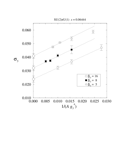
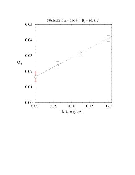
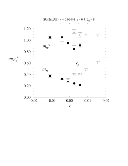
          (a)                                                          (b)

          (c)                                                          (d)

Figure 1: Lattice results for the 3d SU(2)$\times$U(1)+Higgs model (from $\!{}^{{\bf?}}$). (a) The two-peak structure indicating a first order transition. The distance between the two peaks determines the latent heat and the height of the plateau between the peaks the surface tension. (b) The infinite volume extrapolation for the surface tension. (c) The continuum extrapolation for the surface tension. (d) The correlator masses around the transition point.

The results of the lattice simulations for the phase diagram are summarized in Fig. 2 (this figure is actually for the SU(2)+Higgs model without the U(1) factor; the difference is small $\!{}^{{\bf?}}$). The main feature is that at small $x$, there is a first order phase transition which gets weaker as $x$ increases, as predicted by perturbation theory. However, unlike in perturbation theory, the non-perturbative transition line ends at $x\sim 0.11$. To the right of the endpoint, there is no first or second order transition.

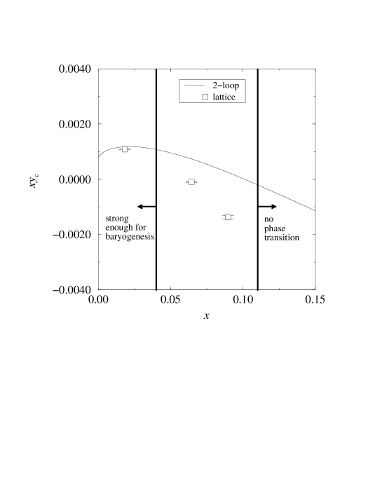
Figure 2: The phase diagram of the 3d SU(2)+Higgs model $\!{}^{{\bf?}}$. The parameters $x,y$ are defined in Sec. 3.2. “Strong enough” refers to the constraint in eq. (14).

In Fig. 2, there is also information about the strength of the transition in the first order regime. Indeed, whether eq. (1) is satisfied or not, depends on the non-perturbative dynamics of the effective theory. It has been shown in $\!{}^{{\bf?}}$ that eq. (1) is satisfied provided that

$$x\mathop{\raise 1.29167pt\hbox{$<$\kern-7.5pt\raise-4.73611pt\hbox{$\sim$}}}0.03\ldots 0.04.$$ (14)

This is a useful result because of its universal character: if there is some other 4d theory than the Standard Model, having the same effective Lagrangian with the same parameter values, then the IR dynamics will be the same! Thus it is sufficient to derive the effective theory perturbatively. The non-perturbative IR-features have already been accounted for by replacing the constraint in eq. (1) by eq. (14).

Finally, one can plug in the values of the 4d physical parameters into the expressions of the 3d parameters. The result is shown in Fig. 3, where also the lattice results from Fig. 2 are included. It is seen that the electroweak phase transition in the Standard Model is never strong enough for baryogenesis. It is of first order, however, for $m_{H}\mathop{\raise 1.29167pt\hbox{$<$\kern-7.5pt\raise-4.73611pt\hbox{$\sim$}}}70-80$ GeV.

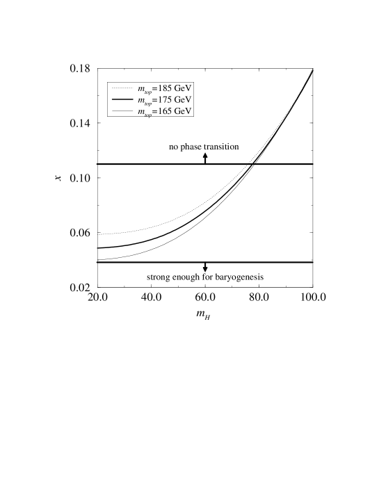
Figure 3: The parameter $x$ determining the strength of the phase transition for the Standard Model, as a function of the pole Higgs mass $m_{H}$ and the pole top mass $m_{\rm top}$ (from $\!{}^{{\bf?}}$).

4 MSSM

Let us then turn to the MSSM. The thermodynamics of the electroweak phase transition in the MSSM has recently been considered perturbatively in $\!{}^{{\bf?}}$${}^{-\,}$$\!{}^{{\bf?}}$. Dimensional reduction has been applied to the MSSM in $\!{}^{{\bf?}}$${}^{-\,}$$\!{}^{{\bf?}}$ (dimensional reduction has recently been applied to a simple GUT-model, as well $\!{}^{{\bf?}}$).

The main observation now is that for a part of the parameter space of the MSSM, the effective theory is the same as in the Standard Model, i.e., given by eq. (7). Then one immediately knows that the IR dynamics is the same, and in particular, that an IR-safe characterization of the strength of the transition can be obtained by computing the parameter $x$. On the other hand, one can also find cases where the IR-dynamics of the transition is more complicated; then another effective 3d theory should be studied on the lattice.

4.1 Reduction to SU(2)$\times$U(1)+Higgs

Let us first see how it could be that the effective theory for the MSSM is just the one given by eq. (7). At first sight, this may not be obvious since the field content of the 4d theory differs quite a lot from the Standard Model. To be more specific, the minimal field content to be considered in the MSSM is that one has two Higgs doublets $H^{1}$, $H^{2}$; the SU(2) and SU(3) gauge fields $A^{a}_{\mu}$, $C^{A}_{\mu}$; the fermionic superpartners of the mentioned fields, i.e., higgsinos and gauginos; quarks of the $3^{\rm rd}$ generation $q_{L},t_{R},b_{R}$; the scalar superpartners of these, i.e., squarks of the $3^{\rm rd}$ generation $Q,U,D$.

To arrive at eq. (7), one now does the following:

• renormalize the vacuum theory analogously to the Standard Model case. Instead of $m_{H}$, the Higgs sector is usually parameterized in terms of $\tan\!\beta$ and the CP-odd Higgs mass $m_{A}$.

• go to finite temperature and integrate out all $n\neq 0$ modes; in particular, all the fermions are integrated out. This removes all the fermionic superpartners (gauginos and higgsinos) from the effective theory.

• integrate out the zero components of the SU(2) and SU(3) gauge fields, $A_{0}$, $C_{0}$, and the heavy squark fields in 3d. In the generic case, all the squark fields are heavy, since the electroweak transition takes place in the Higgs direction. Thus only the gauge fields and two Higgs doublets are left.

• diagonalize the two Higgs doublet model at the transition point where the mass matrix has an eigenvalue close to zero.

• integrate out the heavy Higgs doublet. Since the sum of the mass eigenvalues is $\sim m_{1}^{2}(T)+m_{2}^{2}(T)\sim m_{A}^{2}+cT^{2}$ and since one of the eigenvalues is close to zero, the other Higgs field is heavy (especially if $m_{A}$ is not very small).

As a result, one indeed gets the effective theory in eq. (7).

However, in every new application, one has to be careful with the accuracy of the reduction steps. Let us therefore see what the expansion parameters discussed in eqs. (8), (9) look like for the MSSM.

1. For step 1 of eq. (5), the largest errors of the type in eq. (8) correspond to strong coupling constant and Yukawa corrections:

$$(N_{c}^{2}-1)\frac{g_{S}^{2}}{(4\pi)^{2}}\ll 1,\hskip 14.22636ptN_{c}\frac{h_{t}^{2}}{(4\pi)^{2}}\ll 1.$$ (15)

These should be relatively well under control. It should be noted that this kind of terms appear more frequently in the MSSM than in the Standard Model.

2. For step 1 of eq. (5), eq. (9) corresponds basically to the high-temperature expansion for the fields that are kept in the effective theory. There are many more dimensionful parameters in the MSSM than in the Standard Model, so that one should require

$$\frac{m_{A}^{2}}{(\pi T)^{2}},\frac{m_{Q}^{2}}{(\pi T)^{2}},\frac{m_{U}^{2}}{(\pi T)^{2}},\frac{\tilde{A}_{t}^{2}}{(\pi T)^{2}}\ll 1,\ldots.$$ (16)

If these conditions are not satisfied for some field, then it has to be treated differently. Another part of eq. (9) is that the transition should not be exceedingly strong.

3. For step 2 of eq. (6), the largest errors in eq. (8) correspond again to strong coupling constant and Yukawa corrections. However, in the 3d theory, the mass parameters also appear for dimensional reasons:

$$\frac{h_{t}^{2}T}{\pi m_{U3}},\frac{g_{S}^{2}T}{\pi m_{U3}},\frac{h_{t}^{2}T}{\pi m_{Q3}},\frac{g_{S}^{2}T}{\pi m_{Q3}}\ll 1.$$ (17)

There are also constraints for the mixing parameters, something like

$$\frac{|\mu|}{m_{Q3}},\frac{|{A}_{t}|}{m_{Q3}}\ll 1.$$ (18)

These constraints have been discussed in $\!{}^{{\bf?}}$ (see also Sec. 5 in $\!{}^{{\bf?}}$).

4. For step 2 of eq. (6), eq. (9) is related to the strength of the phase transition and, provided that eq. (17) is satisfied, should be under control unless the transition is exceedingly strong ($v/T\mathop{\raise 1.29167pt\hbox{$>$\kern-7.5pt\raise-4.73611pt\hbox{$\sim$}}}3$), see $\!{}^{{\bf?}}$.

Of these error estimates, the ones first causing problems are eqs. (17), (18). In particular, in the small stop scenario $\!{}^{{\bf?},{\bf?}}$ the mass parameter $m_{U3}$ is small, $m_{U3}\sim 0$, and the first two expansion parameters in eq. (17) break down. Then the $U$-field cannot be integrated out, and one has to go to the treatment in Sec. 4.2. The second problem may be associated with eq. (18) in the case that there is large mixing in the squark sector $\!{}^{{\bf?}}$.

On the other hand, there are certainly cases where the expansion parameters are small. One typical such case is shown in Fig. 4. Here the physical right-handed stop mass is $m_{\widetilde{t_{R}}}^{2}\approx m_{U}^{2}+m_{\rm top}^{2}$, so that $m_{U}\approx 50$ GeV corresponds to $m_{\widetilde{t_{R}}}\approx 180$ GeV. It is seen that one can indeed get a strong enough phase transition if $m_{A}$ is large and $m_{H}\mathop{\raise 1.29167pt\hbox{$<$\kern-7.5pt\raise-4.73611pt\hbox{$\sim$}}}80$ GeV. On the other hand, the transition is getting stronger as $m_{U}$ is becoming smaller, in which limit the reliability of the reduction is decreasing due to the fact $m_{U3}$ in eq. (17) is becoming smaller. However, for $m_{U}=50$ GeV the expansion parameters are still relatively small. Hence the conclusion is that one can have a transition strong enough for baryogenesis for the experimentally allowed Higgs masses, unlike in the Standard Model $\!{}^{{\bf?}}$${}^{-\,}$$\!{}^{{\bf?}}$.

Finally, though not indicated in Fig. 4, it is interesting to note that for these parameters one always gets a first order transition as one increases $\tan\!\beta$ (or $m_{H}$), although the transition is getting weaker. The situation is thus quite different from the Standard Model case, where there is no transition at high enough Higgs masses.

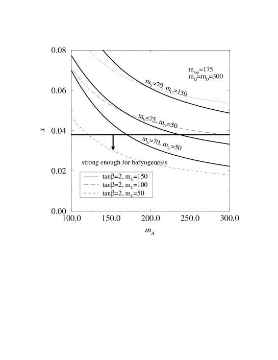
Figure 4: The parameter $x$ in the MSSM, in terms of the CP-odd Higgs mass $m_{A}$, the lightest CP-even Higgs mass $m_{h}$ and the stop mass parameter $m_{U}$ (from $\!{}^{{\bf?}}$). The physical right-handed stop mass is $m_{\widetilde{t_{R}}}^{2}\approx m_{U}^{2}+m_{\rm top}^{2}$, so that $m_{U}\approx 50$ GeV implies $m_{\widetilde{t_{R}}}\approx 180$ GeV.

4.2 Reduction to SU(3)$\times$SU(2)+ two scalars

Let us then consider the light stop scenario. In that case that the right-handed stop cannot be integrated out, since the expansion parameters in eq. (17) would explode. Thus the stop field $U$ has to be kept in the effective theory. The form of the effective 3d theory can be written down, based on gauge invariance $\!{}^{{\bf?}}$:

$${\cal L}_{\rm 3d} = {\frac{1}{4}}F^{a}_{ij}F^{a}_{ij}+{\frac{1}{4}}G^{A}_{ij}G^{A}_{ij}+\gamma_{3}H^{\dagger}HU^{\dagger}U$$ (19)

$$+ (D_{i}^{w}H)^{\dagger}(D_{i}^{w}H)+m_{H3}^{2}H^{\dagger}H+\lambda_{H3}(H^{\dagger}H)^{2}$$

$$+ (D_{i}^{s}U)^{\dagger}(D_{i}^{s}U)+m_{U3}^{2}U^{\dagger}U+\lambda_{U3}(U^{\dagger}U)^{2}.$$

Here $D_{i}^{w}$ and $D_{i}^{s}$ are the SU(2) and SU(3) covariant derivatives, and $F_{ij}^{a}$, $G_{ij}^{A}$ are the corresponding field strengths. The U(1) group was for simplicity neglected. The form in eq. (19) assumes, e.g., that the squark mixing parameters are not exceedingly large.

The values of the parameters in eq. (19) have been computed at 1-loop level in a particular scenario in $\!{}^{{\bf?}}$, with an estimate of the most important 2-loop effects included. It should be stressed that the 2-loop effects are numerically quite important in some cases and a complete 2-loop derivation might be useful if the MSSM parameters turn out to be such that the effective theory in eq. (19) is relevant. This is because the scale of the couplings in the thermal screening terms is fixed only at the 2-loop level as discussed after eq. (12), and for the squark mass parameters where the strong gauge coupling appears, this can have a significant numerical effect.

On the other hand, independent of the accuracy of the reduction steps, it would be quite important to analyze the theory of eq. (19) on the lattice. This is because the IR-modes of eq. (19) are exactly those which are responsible for the strengthening effects seen in $\!{}^{{\bf?}}$${}^{-\,}$$\!{}^{{\bf?}}$. Unfortunately, no lattice results are available at the moment.

In perturbation theory, the possible transitions in the theory of eq. (19) have been studied at the 2-loop level in $\!{}^{{\bf?}}$. Using the reduction formulas for the 3d parameters in terms of 4d physics, one can see that the electroweak phase transition can indeed be quite strong for small right-handed stop masses. Results for the phase diagram and for the constraint of eq. (1) are shown in Fig. 5. It is seen that Higgs masses up to 100 GeV could be allowed and that there might even be the possibility of a two-stage transition.

However, it should be noted that there is a relatively large gauge and scale dependence in the 2-loop results in this regime $\!{}^{{\bf?}}$. Thus, even if the transition is strong (which in the Standard Model case turned out to imply that the IR-problems are not very severe, after all), there is some uncertainty in the perturbative results in the present case and a lattice study is really needed.

Finally, concerning the lattice study, let us note that there are many more parameters in eq. (19) than in eq. (7). In fact, if the strong gauge coupling $g_{S3}^{2}$ is chosen to fix the scale, then there are six dimensionless parameters left. Thus one has in a sense less universality than in eq. (7), and one has to choose somewhat more specific 4d parameter values for the lattice study.

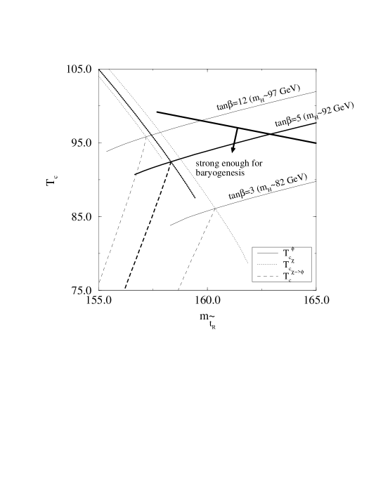
Figure 5: The phase structure of the MSSM with a light stop according to $\!{}^{{\bf?}}$. The solid lines indicate the conventional SU(2) transition, whereas the dotted lines indicate a transition to the colour breaking stop direction. The dashed lines are transitions from the stop direction to the standard SU(2) broken minimum. Within the approximations made and for the parameters used, it thus appears possible, in principle, to have a two-stage transition.

5 Conclusions and Outlook

The method of dimensional reduction allows the construction of effective 3d theories for the electroweak sector of the Standard Model, as well as for many extension thereof. This construction is free of IR-problems and perturbative, and thus at least in the cases where perturbation theory works at zero temperature, one expects the reduction to be reliable. However, one should keep in mind that there are also other expansion parameters involved, especially related to 3d heavy scale integrations. Thus it is important to estimate the accuracy of the reduction steps each time a new theory is studied.

In cases where the expansion parameters of the analytic reduction steps are getting larger, it would, in principle, be nice to have 4d simulations for comparison. The realistic full 4d theory is far too complicated for this, but one might hope that in somewhat simplified models (like the pure 4d SU(2)+Higgs theory for the Standard Model), one could eventually make a meaningful comparison. Moreover, the accuracy of 3d heavy scale integrations could be checked non-perturbatively with 3d simulations in a more complete effective theory, which is still less demanding than full 4d simulations.

Once a 3d theory has been perturbatively constructed, it can be used in a straightforward manner for lattice simulations. Analytically calculated lattice-continuum relations allow an accurate extrapolation to the continuum limit. Thus the IR-problem plaguing direct 4d perturbative computations can be circumvented.

As a result of this program, the thermodynamics of the EW phase transition is now known with a relatively good accuracy for a large class of theories. For the Standard Model, the effective theory is 3d SU(2)+Higgs (neglecting the U(1) group which has small effects), and the transition is too weak for baryogenesis for any $m_{H}$. However, it is of the first order up to $m_{H}\sim 70-80$ GeV.

For the MSSM, the effective theory may be 3d SU(2)+Higgs or more complicated, depending, in particular, on whether $m_{\widetilde{t_{R}}}\mathop{\raise 1.29167pt\hbox{$>$\kern-7.5pt\raise-4.73611pt\hbox{$\sim$}}}180$ GeV or not. For the case $m_{\widetilde{t_{R}}}\mathop{\raise 1.29167pt\hbox{$>$\kern-7.5pt\raise-4.73611pt\hbox{$\sim$}}}180$ GeV leading to eq. (7), the available lattice results apply and baryogenesis is possible up to $m_{H}\mathop{\raise 1.29167pt\hbox{$<$\kern-7.5pt\raise-4.73611pt\hbox{$\sim$}}}m_{W}$. For smaller $m_{\widetilde{t_{R}}}$, the perturbative indications are that the transition could be strong enough up to $m_{H}\mathop{\raise 1.29167pt\hbox{$<$\kern-7.5pt\raise-4.73611pt\hbox{$\sim$}}}100$ GeV and that there may even be the possibility of a two-stage transition. However, one would need to make new lattice simulations to confirm this. That the transition is stronger usually means that perturbation theory is more reliable. However, one has seen a relatively large gauge and renormalization scale dependence in this regime, possibly implying that there are surprises.

References

References

- [1] V.A. Rubakov and M.E. Shaposhnikov, Usp. Fiz. Nauk 166, 493 (1996) [hep-ph/9603208].
- [2] V.A. Kuzmin, V.A. Rubakov and M.E. Shaposhnikov, Phys. Lett. B 155, 36 (1985); M.E. Shaposhnikov, Nucl. Phys. B 287, 757 (1987).
- [3] P. Arnold and L. McLerran, Phys. Rev. D 36, 581 (1987).
- [4] S.Yu. Khlebnikov and M.E. Shaposhnikov, Nucl. Phys. B 308, 885 (1988).
- [5] A.D. Linde, Phys. Lett. B 96, 289 (1980).
- [6] D. Gross, R. Pisarski and L. Yaffe, Rev. Mod. Phys. 53, 43 (1981).
- [7] P. Arnold and O. Espinosa, Phys. Rev. D 47, 3546 (1993); Phys. Rev. D 50, 6662 (1994) (E); Z. Fodor and A. Hebecker, Nucl. Phys. B 432, 127 (1994).
- [8] B. Bunk, E.M. Ilgenfritz, J. Kripfganz and A. Schiller, Phys. Lett. B 284, 371 (1992); Nucl. Phys. B 403, 453 (1993).
- [9] F. Csikor, Z. Fodor, J. Hein, K. Jansen, A. Jaster and I. Montvay, Phys. Lett. B 334, 405 (1994); Z. Fodor, J. Hein, K. Jansen, A. Jaster and I. Montvay, Nucl. Phys. B 439, 147 (1995); F. Csikor, Z. Fodor, J. Hein and J. Heitger, Phys. Lett. B 357, 156 (1995); F. Csikor, Z. Fodor, J. Hein, A. Jaster and I. Montvay, Nucl. Phys. B 474, 421 (1996).
- [10] Y. Aoki, UTCCP-P-20 [hep-lat/9612023].
- [11] Z. Fodor, these proceedings.
- [12] J. Hein, these proceedings.
- [13] M.E. Shaposhnikov, Proceedings of the Summer School on Effective Theories and Fundamental Interactions, Erice, 1996 [hep-ph/9610247].
- [14] P. Ginsparg, Nucl. Phys. B 170, 388 (1980); T. Appelquist and R. Pisarski, Phys. Rev. D 23, 2305 (1981); S. Nadkarni, Phys. Rev. D 27, 917 (1983).
- [15] K. Farakos, K. Kajantie, K. Rummukainen and M. Shaposhnikov, Nucl. Phys. B 425, 67 (1994); K. Kajantie, M. Laine, K. Rummukainen and M. Shaposhnikov, Nucl. Phys. B 458, 90 (1996).
- [16] A. Jakovác, K. Kajantie and A. Patkós, Phys. Rev. D 49, 6810 (1994); A. Jakovác, Phys. Rev. D 53, 4538 (1996); A. Jakovác and A. Patkós, Phys. Lett. B 334, 391 (1994); Nucl. Phys. B 494, 54 (1997).
- [17] S.-Z. Huang and M. Lissia, Nucl. Phys. B 438, 54 (1995).
- [18] E. Braaten, Phys. Rev. Lett. 74, 2164 (1995); E. Braaten and A. Nieto, Phys. Rev. Lett. 73, 2402 (1994); Phys. Rev. D 51, 6990 (1995); Phys. Rev. Lett. 76, 1417 (1996); Phys. Rev. D 53, 3421 (1996); A. Nieto, Int. J. Mod. Phys. A 12, 1431 (1997); these proceedings [hep-ph/9707267].
- [19] M. Laine, Phys. Lett. B 385, 249 (1996).
- [20] K. Kajantie, K. Rummukainen and M. Shaposhnikov, Nucl. Phys. B 407, 356 (1993); K. Farakos, K. Kajantie, K. Rummukainen and M. Shaposhnikov, Phys. Lett. B 336, 494 (1994).
- [21] K. Kajantie, M. Laine, K. Rummukainen and M. Shaposhnikov, Nucl. Phys. B 466, 189 (1996); Phys. Rev. Lett. 77, 2887 (1996).
- [22] K. Kajantie, M. Laine, K. Rummukainen and M. Shaposhnikov, Nucl. Phys. B 493, 413 (1997).
- [23] E.-M. Ilgenfritz, J. Kripfganz, H. Perlt and A. Schiller, Phys. Lett. B 356, 561 (1995); M. Gürtler, E.-M. Ilgenfritz, J. Kripfganz, H. Perlt and A. Schiller, hep-lat/9512022; Nucl. Phys. B 483, 383 (1997); M. Gürtler, E.-M. Ilgenfritz and A. Schiller, UL-NTZ 08/97 [hep-lat/9702020]; UL-NTZ 10/97 [hep-lat/9704013].
- [24] F. Karsch, T. Neuhaus, A. Patkós and J. Rank, Nucl. Phys. B 474, 217 (1996).
- [25] O. Philipsen, M. Teper and H. Wittig, Nucl. Phys. B 469, 445 (1996).
- [26] G.D. Moore and N. Turok, Phys. Rev. D 55, 6538 (1997).
- [27] K. Farakos, K. Kajantie, K. Rummukainen and M. Shaposhnikov, Nucl. Phys. B 442, 317 (1995).
- [28] M. Laine, Nucl. Phys. B 451, 484 (1995).
- [29] M. Laine and A. Rajantie, HD-THEP-97-16 [hep-lat/9705003].
- [30] G.D. Moore, Nucl. Phys. B 493, 439 (1997); hep-ph/9705248.
- [31] M. Carena, M. Quirós and C.E.M. Wagner, Phys. Lett. B 380, 81 (1996).
- [32] D. Delepine, J.-M. Gérard, R. Gonzalez Felipe and J. Weyers, Phys. Lett. B 386, 183 (1996).
- [33] J.R. Espinosa, Nucl. Phys. B 475, 273 (1996).
- [34] M.P. Worah, SLAC-PUB-7417 [hep-ph/9702423].
- [35] B. de Carlos and J.R. Espinosa, SUSX-TH-97-005 [hep-ph/9703212].
- [36] M. Quirós, IEM-FT-152-96 [hep-ph/9703326]; M. Carena and C.E.M. Wagner, FERMILAB-PUB-97-095-T [hep-ph/9704347].
- [37] J.R. Espinosa, these proceedings [hep-ph/9706389].
- [38] M. Laine, Nucl. Phys. B 481, 43 (1996).
- [39] J.M. Cline and K. Kainulainen, Nucl. Phys. B 482, 73 (1996); McGill/97-7 [hep-ph/9705201].
- [40] M. Losada, RU-96-25 [hep-ph/9605266]; G.R. Farrar and M. Losada, RU-96-26 [hep-ph/9612346].
- [41] D. Bödeker, P. John, M. Laine and M.G. Schmidt, Nucl. Phys. B 497, 387 (1997) [hep-ph/9612364].
- [42] J. Cline, these proceedings.
- [43] A. Rajantie, Nucl. Phys. B, in press [hep-ph/9702255]; these proceedings.