hep-ph/9707405

DSF 35/97

SISSA 95/97/EP

Hybrid Inflation from Supersymmetric SU(5)

L. Covi^1,2, G. Mangano³, A. Masiero^1,4, and G. Miele³

¹ International School for Advanced Studies, SISSA-ISAS, Via Beirut 2/4, I-34014,Trieste, Italy
² INFN, Sezione di Trieste, Via A. Valerio 2, I-34127 Trieste, Italy
³ Dipartimento di Fisica, Universitá di Napoli ”Federico II”, and INFN, Sezione di Napoli, Mostra D’Oltremare Pad. 20, I-80125 Napoli, Italy
⁴ Dipartimento di Fisica, Universitá di Perugia, and INFN, Sezione di Perugia, Via Pascoli, I-06123 Perugia, Italy

Abstract

A scheme of hybrid inflation is considered in the framework of the minimal supersymmetric $SU(5)$ model with an extra singlet. The relevant role of the cubic term in the adjoint representation in the renormalizable superpotential is pointed out in order to have a quite wide region of initial conditions compatible with inflation efficiency, monopole density dilution and perturbations constraint.

PACS number(s):12.60.Jv; 98.80.Cq

Unified gauge theories certainly provide a natural framework where to look for a proper scalar dynamics able to drive inflation. The debate on the inflationary option to adopt to match the most recent observations is still open [1]-[5]. A particularly attractive scenario is hybrid inflation [5]. In this class of models, by using more than one scalar field, one naturally overcomes the unpleasant feature to have an incredibly small coupling constant, typical of single scalar field models [6]. As far as the elementary particle physics is concerned, supersymmetric GUT models still remain one of the most appealing candidates for next step in unification programme [7], and naturally provide many scalar fields. The simplest GUT example capable to unify all gauge interactions is the supersymmetric $SU(5)$ model [8].

There already exist some examples of simplified SUSY hybrid realizations [6]. Here we intend to construct a hybrid inflationary scheme based on a realistic SUSY $SU(5)$ model with an additional singlet superfield. In particular we will show that it is possible to avoid a characteristic problem of such approaches, an excessive production of magnetic monopoles at the end of inflation.

Let us consider the following globally supersymmetric renormalizable superpotential

$$W=\mu^{2}~{}s-\alpha~{}s~{}\hbox{{\rm Tr}}(\Phi^{2})-\beta\hbox{{\rm Tr}}(\Phi^{3})+\gamma~{}\overline{H}\Phi H+\delta~{}\overline{H}H~{}~{}~{},$$ (1)

where $s$ is a complex gauge singlet field, $\Phi$ denotes a complex $\underline{24}$ irreducible representations (IRR) of $SU(5)$, and $H_{a}$ and $\overline{H}_{a}$, with $a=1,..5$, stand for a $\underline{5}$ and $\underline{\overline{5}}$ IRR’s of $SU(5)$, respectively. Without loss of generality we can choose $\mu^{2},\alpha,\beta$ as positive real constants by a suitable redefinition of complex fields. We can express $\Phi$ in components with respect to the $SU(5)$ adjoint basis $\Phi=\phi_{i}T^{i}$. We will denote with the same letter the chiral superfields or its scalar component depending on the context. For simplicity we omit higher order terms in $s$.

In terms of components, the superpotential becomes

$$W=\mu^{2}~{}s-{\alpha\over 2}~{}s~{}\Sigma_{i=1}^{24}\phi_{i}^{2}-{\beta\over 4}d_{ijk}\phi_{i}\phi_{j}\phi_{k}+\gamma T^{i}_{ab}~{}\overline{H}_{a}\phi_{i}H_{b}+\delta\overline{H}_{a}H_{a}~{}~{}~{},$$ (2)

where $d_{ijk}\equiv 2\hbox{{\rm Tr}}(T^{i}\{T^{j},T^{k}\})$. Using Eq. (2) one gets the potential for the scalar components of the Higgs superfields $s$, $\Phi$, $H$ and $\overline{H}$

$$V\left(s,\Phi,H,\overline{H}\right)=\left|\mu^{2}-{\alpha\over 2}~{}\Sigma_{i=1}^{24}\phi_{i}^{2}\right|^{2}+\Sigma_{i=1}^{24}\left|\alpha s\phi_{i}+{3\beta\over 4}d_{ijk}\phi_{j}\phi_{k}-\gamma T^{i}_{ab}\overline{H}_{a}H_{b}\right|^{2}$$

$$+\Sigma_{b=1}^{5}\left(\left|\gamma T^{i}_{ab}\phi_{i}\overline{H}_{a}+\delta\overline{H}_{b}\right|^{2}+\left|\gamma T^{i}_{ba}\phi_{i}H_{a}+\delta H_{b}\right|^{2}\right)+(D-\mbox{terms})~{}~{}~{}.$$ (3)

Then the absolute minimum of the supersymmetric potential results to be

$$\Sigma_{i=1}^{24}(\phi^{0}_{i})^{2}={2\mu^{2}\over\alpha}~{}~{}~{},~{}~{}H^{0}_{a}~{}=~{}\overline{H}^{0}_{a}=0~{}~{}~{},~{}~{}~{}s^{0}=-{3\beta\over 8\mu^{2}}d_{ijk}\phi^{0}_{i}\phi^{0}_{j}\phi^{0}_{k}~{}~{}~{}.$$ (4)

We can always use an $SU(5)$ transformation to put the v.e.v. matrix $\Phi^{0}$ into diagonal form, $\phi^{0}_{i}\neq 0$ only along the four Cartan diagonal generators. The request $\phi^{0}_{j}=\phi^{0*}_{j}$ for such components both ensures vanishing D-terms and verifies the first condition of Eq. (4) where the r.h.s. is positive. The superscript $0$ reminds that the background configurations correspond to the absolute minimum.

To realize the $SU(5)$ breaking into $SU(3)_{C}\otimes SU(2)_{L}\otimes U(1)_{Y}$, all $\phi_{i}$ will vanish apart of $\phi_{8}\equiv v/\sqrt{2}$ (hypercharge component) and $s\equiv\sigma/\sqrt{2}$ ($v$ and $\sigma$ two real scalar fields). Thus, by virtue of (4) one has two possible solutions:

$$v^{0}=\pm{2\mu\over\sqrt{\alpha}}~{}~{}~{}\mbox{and}~{}~{}~{}\sigma^{0}=\pm{3\beta\mu\over\sqrt{60}\alpha^{3/2}}~{}~{}~{}\mbox{accordingly}.$$ (5)

The parameters $\mu$ and $\alpha$ of our superpotential are therefore connected to the Higgs expectation value.

As usual to have doublet-triplet splitting in $H$ and $\overline{H}$, a fine tuning on the potential parameters is required. Let us denote by $h_{3}$ ($\overline{h}_{3}$) and $h_{2}$ ($\overline{h}_{3}$) the above triplet and doublet components of $H$ ($\overline{H}$). By using the expression (3) for the potential $V$, evaluated at the absolute supersymmetric minimum (4), one gets the following mass terms

$$\left(\delta+{\gamma v^{0}\over\sqrt{30}}\right)^{2}\left(h_{3}^{{\dagger}}h_{3}+\overline{h}_{3}\overline{h}_{3}^{{\dagger}}\right)+\left(\delta-{3\gamma v^{0}\over 2\sqrt{30}}\right)^{2}\left(h_{2}^{{\dagger}}h_{2}+\overline{h}_{2}\overline{h}_{2}^{{\dagger}}\right)~{}~{},$$ (6)

where $v^{0}$ has one of the values in Eq. (5). Thus, in order to have the doublets massless one has to impose the fine tuning condition

$$\delta={3\gamma v^{0}\over 2\sqrt{30}}~{}~{}~{}.$$ (7)

Let us now consider the inflationary scenario emerging in the framework of our model, with chaotic initial conditions. According to this picture, the initial values for $\Phi$ and $s$, emerging from the quantum cosmological period, are arbitrary, and in general do not coincide with the supersymmetric absolute minima (5). For simplicity we will assume however that the direction of this fields is already $SU(3)_{C}\otimes SU(2)_{L}\otimes U(1)_{Y}$ invariant, and it remains so during all the evolution. This is a simplifying assumption since one should consider a general $SU(5)$ breaking and follow the dynamics of all the independent fields without fixing a preferred direction. At the moment our goal is to see if it is possible to have a viable inflationary scenario in the context of a simplified SUSY $SU(5)$ model.

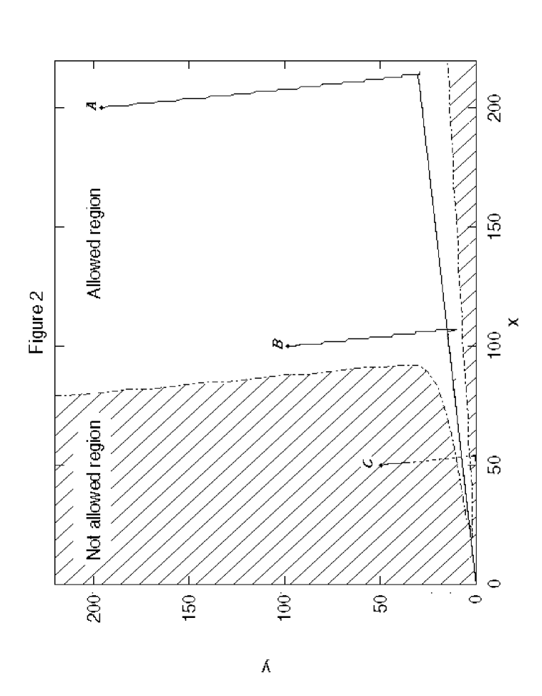
Figure 2: The curves A,B and C start from different initial conditions $(x_{i},y_{i})$, respectively, from the right, (200,200), (100,100), (50,50). The first two correspond to $N=150$ and $40$, respectively. The third one falls into the symmetric $SU(5)$ potential valley. The shaded region contains the initial conditions leading to $SU(5)$ symmetry restoration during the inflationary dynamics.

The consistency of our assumption requires at least that the chosen direction should be locally stable with respect to small perturbations in any other direction, as for example the one invariant under $SU(4)\otimes U(1)$. This is actually the case, since we have verified that all the above perturbations have positive mass square in the region $v$–$\sigma$ we are going to study (see later Fig. 2).

In terms of the real scalar fields $v$ and $\sigma$, the classical potential of Eq.(3) becomes

$$V\left(\sigma,v\right)=\left(\mu^{2}-{\alpha\over 4}v^{2}\right)^{2}+{\alpha^{2}\over 4}v^{2}\left(\sigma-\xi v\right)^{2}~{}~{}~{},$$ (8)

where $\xi\equiv 3\beta/(2\sqrt{60}\alpha)$.

Let us for convenience rewrite the potential in terms of adimensional variables rescaling all the fields with respect to $v^{0}$ and the scalar potential with respect to the mass scale $\mu$:

$$y = {\sqrt{\alpha}\over 2\mu}v~{}~{}~{},~{}~{}~{}~{}~{}~{}~{}~{}x={\sqrt{\alpha}\over 2\mu}\sigma~{}~{}~{},$$ (9)

$$\widetilde{V} = {V\over\mu^{4}}=(1-y^{2})^{2}+4y^{2}(x-\xi y)^{2}~{}~{}~{}.$$ (10)

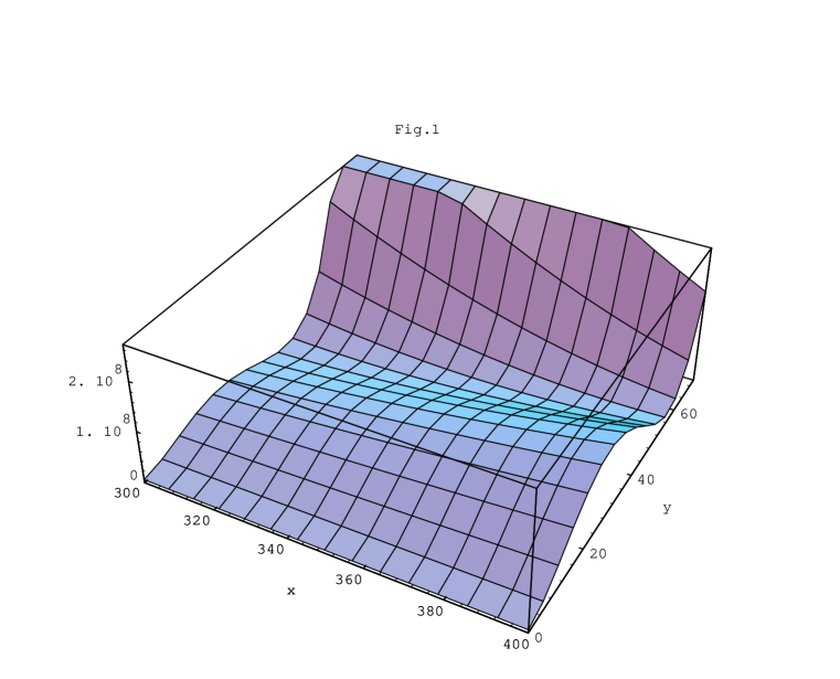
Figure 1: The dimensionless potential $\widetilde{V}$ for $\xi=7$ is here shown.

In Fig. 1 we show the potential for a particular value of $\xi$. We can see that it is characterized by two valleys, one corresponding to $y=0$ ($SU(5)$ symmetric configuration) and the other with $x=\xi y$. It is interesting to notice that although the second valley displays for large values of $x$ a higher energy density with respect to the first one, it is exactly the second pointing toward the supersymmetric minimum.

In terms of these quantities, the early universe scalar dynamics reads

$$\ddot{y} + 3\widetilde{H}\dot{y}+{\delta\widetilde{V}\over\delta y}=0~{}~{}~{},$$ (11)

$$\ddot{x} + 3\widetilde{H}\dot{x}+{\delta\widetilde{V}\over\delta x}=0~{}~{}~{},$$ (12)

$$\dot{N} = \widetilde{H}=K\left[{\dot{y}^{2}\over 2}+{\dot{x}^{2}\over 2}+\widetilde{V}\right]^{1/2},$$ (13)

where $K$ is defined as $\sqrt{32\pi\mu^{2}/(3\alpha M_{Pl}^{2})}$ and $N$ denotes the e-foldings. In the previous equations the dot indicates the derivative with respect to the dimensionless time $\tau=t\mu\sqrt{\alpha}/2$ and also the Hubble parameter $\widetilde{H}$ is properly rescaled. Notice that all the dynamics depends only on the initial conditions and on the parameters $K$ and $\xi$.

We can proceed to a numerical integration of Eq. (13) to obtain the classical dynamics of the fields starting with arbitrary initial conditions $x_{i}$ and $y_{i}$. Depending on the initial values we have observed that two possible dynamics take place: in one case the fields enter the $SU(5)$ symmetric valley and the symmetry is restored during the inflationary period to be broken later at the end of inflation. We have then production of monopoles that cannot be diluted by a sufficiently large e-foldings. On the contrary, for other initial conditions, the symmetry is no more restored and the fields slowly descend toward the supersymmetric minimum along the valley $x=\xi y$. In this case any topological defects production took place before inflation and can be efficiently diluted. In Fig. 2 we show some trajectories in the $x-y$ plane for particular initial conditions. The lines starting at A and B correspond to large initial conditions and, as can be seen clearly, both follow the second valley of the potential up to the supersymmetric minimum. They yield a large number of e-foldings, 150 and 40 respectively. On the contrary line C describes a situation in which the fields fall in the $SU(5)$ symmetric valley until practically the end of inflation. In Fig. 2 are well indicated for positive $x$ and $y$ (the case of both negative $x$ and $y$ is completely analogous) the two regions of initial conditions corresponding to the two described behaviour. For $x_{i}>0$ and $y_{i}<0$ or viceversa the dynamics proceeds towards symmetry restoration and is therefore not favorable.

The field behaviour for lines A and B in Fig. 2 can be understood qualitatively looking at the dynamics in the directions singled out by the valley (one orthogonal and the other along the bottom of the valley); defining:

$$z={x-\xi y\over\sqrt{1+\xi^{2}}}~{}~{}~{},~{}~{}~{}~{}w={y+\xi x\over\sqrt{1+\xi^{2}}}~{}~{}~{},$$ (14)

we have that the gradient of the potential is given by

$${\delta\widetilde{V}\over\delta z} = 8z(w-\xi z)^{2}-8\xi z^{2}(w-\xi z)+{4\xi\over 1+\xi^{2}}(w-\xi z)(1-{(w-\xi z)^{2}\over 1+\xi^{2}})~{}~{}~{},$$ (15)

$${\delta\widetilde{V}\over\delta w} = 8z^{2}(w-\xi z)-{4\over 1+\xi^{2}}(w-\xi z)(1-{(w-\xi z)^{2}\over 1+\xi^{2}})~{}~{}~{}.$$ (16)

It is easily seen from these expressions that the force along the $z$ direction is greater than the one along $w$ for $\xi$ larger than unity and all choices of initial conditions corresponding to a negative $z_{i}$ and large $w_{i}$ (i.e. large $x_{i}\simeq y_{i}$), since Eq. (16) is suppressed by a factor $1/\xi$ with respect to part of Eq. (15). The r.h.s. of Eq. (15) is large and negative and pushes $z$ to zero; correspondingly we will have first an essentially one-dimensional motion along $z$ and then an analogous behavior along $w$ for $z=0$.

The parameter $\xi$ affects only the first part of the dynamics; it must be sufficiently large to have well separated valleys defined by $x=\xi y$ and $y=0$. In this case $\xi$ rules the velocity of approaching from the initial point the bottom of the valley. Fundamental in stopping the fields in the valley is the strength of the frictional term proportional to $K$. The second part of dynamics, now independent of $\xi$, is only affected by $K$. Again the friction term must be large enough to slow down the fields so that they do not overcame the $y=0$ barrier separating the minima at $y=\pm 1$, and start small oscillations around the supersymmetric minimum. Interestingly the numerical analysis shows that an acceptable behaviour is obtained for $K\geq 7\cdot 10^{-2}$.

Whenever $K$ is chosen in this range, the initial conditions for $x$ and $y$ cannot be chosen too small as indicated by the shaded region in Fig. 2. Apart from this bound, starting in the allowed region, to small initial conditions correspond small e-folding.

For the $SU(5)$ asymmetric dynamics, we have an initial inflationary period while $z$ is approaching zero and then a second stage of inflation during the motion along the valley. For very special initial condition both phases of inflation are necessary to give the $60$ e-folds able to solve the smoothness problem, and in this case the computation of the scalar density perturbation is more involved [9]. However the second stage of inflation is generally long enough to produce an e-fold number of the order of $100$ and then it is possible to compute the scalar density perturbation neglecting the previous history. The dynamics along $w$ fairly satisfies slow roll conditions; by considering the potential along the bottom of the valley as a function of $w$, one can easily estimate the slow-roll parameters $\epsilon$ and $\eta$ [10]

$$\epsilon = {1\over 6K^{2}}\left({\widetilde{V}^{\prime}\over\widetilde{V}}\right)^{2}\leq 0.3\cdot 10^{2}\left({\widetilde{V}^{\prime}\over\widetilde{V}}\right)^{2}~{}~{}~{},$$ (17)

$$\eta = {1\over 3K^{2}}{\widetilde{V}^{\prime\prime}\over\widetilde{V}}\leq 0.6\cdot 10^{2}{\widetilde{V}^{\prime\prime}\over\widetilde{V}}~{}~{}~{},$$ (18)

where the primes denote the derivatives with respect to the $w$ variable and the bounds are given considering the bound on $K$ due to the dynamics. Both the quantities depending on the potential are smaller than $1$ for $w\geq 30$, i.e. the slow roll conditions break down only when the fields approach the supersymmetric minimum $w=\sqrt{1+\xi^{2}}$. In particular the value $w_{e}$ at which the inflation ends is given by $\max\{\epsilon,|\eta|\}=1$.

Since along the valley the dynamics is effectively one-dimensional and satisfies the slow roll conditions, we can also easily evaluate the cosmic background radiation quadrupole anisotropy [11]. The limit on scalar density fluctuations gives

$$\left({\Delta T\over T}\right)_{Q}\simeq\sqrt{32\pi\over 45}\left|{V^{3/2}\over V^{\prime}M^{3}_{Pl}}\right|_{w_{Q}}={2K\over\sqrt{15}}\left({\mu\over M_{Pl}}\right)^{2}\left({\widetilde{V}^{3/2}\over\widetilde{V}^{\prime}}\right)_{w_{Q}}\leq 7\cdot 10^{-6}~{}~{}~{},$$ (19)

where the subscript $w_{Q}$ indicates the value of $w$ as the scale, which evolved to the present horizon size, crossed out the horizon during inflation. The e-folding evaluated from $w_{Q}$ till the end of the inflation, $w=w_{e}$, is of the order of $N(w_{Q})\simeq 60$.

From Eq.s (17) and (18) we easily get for $w_{e}$

$$w_{e}^{2}=1+\xi^{2}+{2\over K^{2}}+{2\over K^{2}}\sqrt{1+{2\over 3}(1+\xi^{2})K^{2}}~{}~{}~{},$$ (20)

and for the e-folding $N(w_{Q})$

$$N(w_{Q})=\frac{3}{8}K^{2}\left[w_{Q}^{2}-w_{e}^{2}-(1+\xi^{2})\log\left({w_{Q}^{2}\over w_{e}^{2}}\right)\right]~{}~{}~{},$$ (21)

which implicitely provides $w_{Q}$ as function of $K$ and $\xi$ only.

The background radiation quadrupole anistropy can therefore be expressed as

$$\left({\Delta T\over T}\right)_{Q}\simeq{3\over 64\pi\sqrt{15}}\alpha K^{3}{(1+\xi^{2}-w_{Q}^{2})^{2}\over(1+\xi^{2})w_{Q}}~{}~{}~{}.$$ (22)

which using the COBE experimental value turns into a value for $\alpha$ depending on $K$ and $\xi$. Actually, using Eq.s (20) and (21) one finds that $\alpha$ is a very slowly varying function, and in particular $\alpha\simeq 1\div 5\cdot 10^{-5}$ for $.1\leq K\leq 1$ and $1\leq\xi\leq 10$.

The bound on $K$ can be also expressed as a lower limit on the mass $m_{V}$ of heavy vector bosons

$${m_{V}\over M_{Pl}}=g_{5}~{}\sqrt{{5\over 32\pi}}K\geq g_{5}~{}1.6~{}10^{-2}~{}~{}~{},$$ (23)

with $g_{5}$ the $SU(5)$ gauge coupling constant, which is fairly compatible with present estimates which take into account threshold effects [12]– [14].

Using the allowed values for $\alpha$ one can also evaluate the masses of colour octet and weak triplet components of the adjoint Higgs. From the expression of the potential, expanded around the absolute SUSY minimum one gets

$${m_{\Phi}\over M_{Pl}}=\sqrt{15\over 32}{\beta v^{0}\over M_{Pl}}=\sqrt{75\over 16\pi}\xi\alpha K$$ (24)

which, for $\xi\sim 1\div 10$ are of the order of $10^{13}\div 10^{15}$ GeV. Indeed such values are lower than the GUT scale, but consistent with those required in [12]–[15] . Our scenario beautifully agrees with such case and displays a high value for leptoquark gauge boson mass, of the order of $10^{17}$ GeV, which is consistent with the unification of coupling prediction only for low values of the Higgs octet and triplet masses $m_{\Phi}$.

A final remark on the spectral index for scalar perturbations. In the slow–roll limit one has

$$n(w_{Q})=1+2\eta(w_{Q})-6\epsilon(w_{Q})$$ (25)

which using Eq.s (17), (18) and (21) gives $n(w_{Q})\sim 0.96$ for $.1\leq K\leq 1$, a result which is compatible with present determinations.

In this letter we have shown how a hybrid inflationary scenario can be successfully realized in the framework of a realistic model based on $SU(5)$ supersymmetric gauge theory, which represents one of the best candidates to describe fundamental interactions up to very large scales beyond the Standard Model. Actually starting from a renormalizable potential, the customary Higgs content of MSSM $SU(5)$ with only an extra singlet, as first considered in a toy model in [6], it is possible to obtain large e-fold number and compatibility with scalar perturbation limits coming from COBE data. In particular the production of monopoles at the symmetry breaking occurs before the inflationary stage for a quite wide range of initial conditions for the scalar fields, so their density is strongly diluted in these cases. Finally no fine tuning of coupling constant is needed in order to fit with cosmological constraints.

We thank G. Dvali, G. Lazarides and Q. Shafi for useful discussions. The work of A.M. was partially supported by the EU contract ERBFMRX CT96 0090.

References

- [1] A.H. Guth, Phys. Rev. D23 (1981) 347.
-
[2]
A.D. Linde, Phys. Lett. B108 (1982) 389.
A. Albrecht and P.J. Steinhardt, Phys. Rev. Lett. 48 (1982) 1220. - [3] A.D. Linde, Phys. Lett. B129 (1983) 177.
-
[4]
D. La and P.J. Steinhardt, Phys. Rev. Lett. 62 (1989)
376.
E.W. Kolb, Physica Scripta T36 (1991) 199.
A.M. Green and A.R. Liddle, Phys. Rev. D54 (1996) 2557. - [5] A.D. Linde, Phys. Lett. B259 (1991) 38; Phys. Rev. D49 (1994) 748.
-
[6]
G. Dvali, Q. Shafi and R. Schaefer, Phys. Rev. Lett. 73 (1994) 1886.
G. Lazarides, R.K. Schaefer and Q. Shafi, Phys. Rev. D56 (1997) 1324. - [7] R.N. Mohapatra, Unification and Supersymmetry, (Springer Verlag, Heidelberg, 1986).
-
[8]
S. Dimopoulos and H. Georgi, Nucl. Phys. B193
(1981) 150.
N. Sakai, Z. Phys. C11 (1981) 153. - [9] J. Silk and M. S. Turner, Phys. Rev. D35 (1987) 419.
- [10] E.J. Copeland, E.W.Kolb, A.R. Liddle and J.E. Lidsey, Phys. Rev. D48 (1993) 2529.
- [11] A.R. Liddle and D.H. Lyth, Phys. Rep. 231 (1993) 1.
- [12] J. Hisano, T. Moroi, K. Tobe and T. Yanagida, Mod. Phys. Lett. A10 (1995) 2267.
- [13] A. Dedes, A.B Lahanas, J. Rizos and K. Tamvakis, Phys. Rev. D55 (1997) 2955.
- [14] N.V. Krasnikov, Phys. Lett. B392 (1997) 365.
- [15] J. Hisano, H. Murayama and T. Yanagida, Phys. Rev. Lett. 69 (1992) 1014.