hep-ph/9707367

NORDITA 97/58

July 1997

revised version

Resummation of $(-b_{0}\alpha_{s})^{n}$ corrections to the photon-meson transition form factor $\gamma^{\ast}+\gamma\rightarrow\pi^{0}$

P. Gosdzinsky^a and N. Kivel^b

^aNORDITA, Blegdamsvej 17, DK-2100 Copenhagen Ø, Denmark

^bPetersburg Nuclear Physics Institute, 188350, Gatchina, Russia

We have resummed all the $(-b_{0}\alpha_{s})^{n}$ contributions to the photon-meson transition form factor $F_{\pi\gamma}$. To do this, we have used the assumption of ‘naive nonabelianization’ (NNA). Within NNA, a series in $(N_{f}\alpha_{s})^{n}$ is interpreted as a series in $(-b_{0}\alpha_{s})^{n}$ by means of the restoration of the full first QCD $\beta$-function coefficient $-b_{0}$ by hand. We have taken into account corrections to the leading order coefficient function and to the evolution of the distribution function. Due to conformal symmetry constraints, it is possible to find the eigenfunctions of the evolution kernel. It turns out that the nondiagonal corrections are small, and neglecting them we obtained a representation for the distribution function with multiplicatively renormalized moments. For a simple shape of the distribution function, which is close to the asymptotic shape, we find that the radiative correction decrease the LO by $30\%$, and the uncertainty in the resummation lies between $10\%$ and $2\%$ for $Q^{2}$ between 2 and 10 GeV².

1 Introduction

We can expect that perturbative QCD (pQCD) works well to describe the process
$\gamma^{*}(q1)\gamma(q2)\rightarrow\pi^{0}$ for accessible values of $q_{1}^{2}<0$ and $q_{2}^{2}\leq 0$. The form factor for this process is given by [2]

$$F_{\pi\gamma}=\int_{0}^{1}\varphi_{\pi}(x,\mu^{2}){\cal C}(x,q_{1},q_{2},\mu^{2})dx+\ldots{}$$ (1)

The leading term in a $1/Q^{2}$ expansion, being $Q^{2}$ the momentum transfer, is given by the integral in (1). The dots, $\ldots$, stand for higher twist contributions, which are subleading in the $1/Q^{2}$ expansion.

The coefficient function ${\cal C}(x,q_{1},q_{2})$, which accounts for the transition from photons to quarks, can be completely described within pQCD. It is known to one loop, and a detailed analysis can be found for example in [3, 4, 5].

The distribution function $\varphi(x,\mu^{2})$ can be interpreted as the transition probability of a $\pi^{0}$ with momentum $P$ into two quarks with momenta $xP$ and $(1-x)P$ respectively. Only its evolution with $\mu^{2}$ is given by pQCD, but not its shape, or $x$ dependence. Here, the situation is rather unclear, and there exist contradictory statements in the literature. Due to our present inability to extract it directly from experiment, we can only make some choice, (or guess) for $\varphi(x,\mu^{2})$. The two most popular choices are the “asymptotic wave function”, $\varphi_{as}=6x(1-x)$, and the CZ model, $\varphi_{CZ}=30x(1-x)(1-2x)^{2}$. Very recently, new experimental data have appeared, and more are expected, [6]. It is expected that this will allow to constrain, and perhaps even extract with some accuracy, the distribution function $\varphi(x,\mu^{2})$. In fact, one of the major goals of the study of the form factor $F_{\pi\gamma}$ is precisely to obtain more information on the distribution function.

In order to extract as much information as possible from the experimental data, precise theoretical predictions for the coefficient function, beyond the one loop level, are needed, and it might even be necessary to include nonleading contributions in the $1/Q^{2}$ counting. In this work, we analyze the accuracy within which the leading order in $1/Q^{2}$, that is, the integral in (1), can predict the form factor $F_{\pi\gamma}$ within Naive Nonabelianization, NNA.

The idea of NNA is based on the observation that corrections related to the evolution with the coupling can represent a source of potentially large perturbative coefficients. The extraction of these large contributions can give important information on higher order corrections. In QCD, this extraction can be done by evaluating the relevant feynman diagrams to leading order in the large $N_{f}$ limit, and interpreting the series in $(N_{f}\alpha_{s})$ as a series in $(-b_{0}\alpha_{s})$, restoring the full QCD $\beta$-function coefficient $-b_{0}$ by hand . Techniques to perform a summation of these large coefficients have been developed in [7, 8].

In this work, we will only calculate leading twist corrections, and use the ultraviolet dominance assumption [9] to estimate the higher twist corrections. This assumption is based on the observation that due to the (infrared) renormalon ambiguity, the leading twist result is affected by an intrinsic ambiguity,

$$\delta C_{LT}\ \ \ \alpha\ \ \ A(y)\left({\Lambda\over Q}\right)^{2}\,{}$$ (2)

where $A(y)$ is a calculable function that is completely fixed by the residues of the Borel integrand, see below, and $y$ denotes the variables on which it depends. The ambiguity in (2) is cancelled by another (ultraviolet) renormalon ambiguity in the higher twist contributions. According to the ultraviolet dominance assumption, not only the ambiguity, but the whole higher twist contribution is proportional to $A(y)$.

This work is organized as follows: In the next section, we briefly review the current state of art. In section 3, we compute the coefficient function within NNA. We find that the coefficient function has two $IR$-renormalon poles and that when one of the photons is on shell, there are additional ambiguities coming from the region $x\rightarrow 0$ and $x\rightarrow 1$. These new ambiguities, which are related to the infrared region, lead to new power corrections to the form factor. In section 4, the NNA evolution kernel is presented. We obtain an expansion for the distribution function in series of Gegenbauer polynomials with the upper index shifted by $b_{0}\alpha_{s}$. We find that the nondiagonal part of the anomalous dimension matrix in this basis is much smaller than the diagonal part. In a first approximation, we can neglect these nondiagonal terms, obtaining multiplicatively renormalized moments. In section 4, we also present two models for the wave functions, and make some comments on the implications that conformal symmetry has. In section 5 we obtain the final result for the form factor in the NNA approximation. We present some numerical results for a simplified distribution function, where only the first term of the expansion is kept. In this case, the shape of the distribution function is close to the asymptotic one. In section 6 we present our conclusions, and finally, we present two appendices with technical details of the calculations.

2 The meson–photon transition form factor

The transition from two photons to a $\pi^{0}$ meson,

$$\gamma^{\ast}(q_{1})+\gamma(q_{2})\rightarrow\pi^{0}(P)$$ (3)

is described by the amplitude $T$

$$T=e^{\alpha}(q_{1})e^{\beta}(q_{2})4\epsilon_{\alpha\beta\lambda\rho}P^{\lambda}\frac{1}{2}(q_{1}-q_{2})^{\rho}F_{\pi\gamma}(Q^{2},\omega).$$ (4)

Here, $F_{\pi\gamma}(Q^{2},\omega)$ is the photon–meson form factor, $e^{\alpha}(q_{1})\ \mbox{and}\ e^{\beta}(q_{2})$ are the polarizations of the colliding photons,  $\ P=q_{1}+q_{2},\ -q_{1}^{2}>0,\ -q_{2}^{2}\geq 0,\ \ Q^{2}=-(q_{1}-q_{2})^{2}/4\ \mbox{and}\ \omega=(q_{1}^{2}-q_{2}^{2})/(q_{1}^{2}+q_{2}^{2})\leq 1$ is the parameter of asymmetry of the photons. If one of the photons ($\gamma_{2}$) is real, $q_{2}^{2}\ =\ 0$ and $\omega\ =\ 1$. In experimentally accessible regions $\omega$ is very close to one.

In fig.1 we have represented the process diagrammatically. The dominant contribution is given by fig1.1, where a large virtual momentum flows through the subgraph containing the two photon vertices. The other regimes correspond to a long distance propagation in the $q_{2}$ channel [10]. The second regime corresponds to the case where the large momentum flows through the central block containing a large virtual photon fig.1.2. The third regime represents the situation when one of the quarks absorbs a large virtual momentum and carries almost all the momentum of the hadron and the second quark is soft, fig.1.3. Power counting predicts that the leading order for these contributions is $1/Q^{4}$. While for $\omega\sim 1$ all three regimes are important, only the first one is relevant for the situation in which both photons are off shell, $\omega<1$. We will now discuss this contribution.

Figure 1: The three regimes of that contribute to the process we are considering

For large $Q^{2}$, the form factor $F_{\pi\gamma}(Q^{2},\omega)$ can be expressed as the convolution of the coefficient function $C(x,\omega,Q,\mu)$ and the distribution function $\varphi(x,\mu^{2})$

$$F_{\pi\gamma}(Q^{2},\omega)\ =\frac{N}{Q^{2}}\int^{1}_{0}C(x,\omega,Q^{2},\mu^{2})\varphi(x,\mu^{2})dx\ \equiv\frac{N}{Q^{2}}C(x,\omega,Q^{2},\mu^{2})\otimes\varphi(x,\mu^{2}),{}$$ (5)

Here, $N=f_{\pi}(e^{2}_{u}-e^{2}_{d})$ is a normalization factor, $e_{q}$ are the chargers of the quarks, $\mu^{2}$ is the renormalization mass, or the scale that separates large from short distances, and $f_{\pi}$ is the pion decay constant, normalized to $f_{\pi}=130$ MeV, see for example [11]. The coefficient function can be calculated in perturbation theory from the hard parton subprocess $\gamma^{\ast}+\gamma^{\ast}\rightarrow q\bar{q}$. At present, the coefficient function is known to leading twist to one loop accuracy, and in the limit $\omega=1$ it has the simple form [4]

$$C(x,Q^{2},\mu^{2})\ =\ \frac{1}{2x}\left(1+\frac{\alpha_{s}}{4\pi}C_{F}\left[\ln\left[\frac{2Q^{2}}{\mu^{2}}\right](3+2\ln x)+\ln x^{2}-\ln\bar{x}-9\right]\right)\ +\{x\leftrightarrow{\bar{x}}\}.{}$$ (6)

with $\bar{x}=1-x$. The distribution function can be determined by the moments

$$f_{\pi}\int\limits^{1}_{0}x^{k}\varphi(x,\mu^{2})dx\ =\ \frac{i^{k}}{(Pn)^{k+1}}\ \langle 0|\bar{d}\gamma_{5}(\hat{n})(Dn)^{k}u|P\rangle{}$$ (7)

where $n_{\mu}$ is a light-like vector, $\hat{n}=\gamma_{\mu}n^{\mu}$, $D_{\mu}$ the covariant derivative and $|P\rangle$ the $\pi^{0}$ meson state with momentum $P$. By definition, $\varphi(x,\mu^{2})$ is normalized to one, $\int\limits^{1}_{0}\varphi(x,\mu^{2})dx\ =\ 1,$ and G-parity implies the relation $\varphi(x)=\varphi(1-x)$. Its $\mu^{2}$ dependence is described by the evolution equation

$$\left[\mu^{2}\frac{\partial}{\partial{\mu^{2}}}+\beta(\alpha_{s})\frac{\partial}{\partial\alpha_{s}}\right]\varphi(x,\mu^{2})\ =\int^{1}_{0}V(x,y|\alpha_{s})\varphi(y,\mu^{2})dy{}$$ (8)

with some initial condition

$$\varphi(x,\mu^{2}_{0})\ =\ \varphi_{0}(x)$$ (9)

The kernel $V(x,y|\alpha_{s})$ is calculable in pQCD, and can be expanded in series of $\alpha_{s}$:

$$V(x,y|\alpha_{s})=\frac{\alpha_{s}}{4\pi}V^{(1)}(x,y)+\left(\frac{\alpha_{s}}{4\pi}\right)^{2}V^{(2)}(x,y)+\cdots$$ (10)

It is known to two loop accuracy [12], [13]. In the one loop approximation [14]:

$$V^{(1)}(x,y) = 2C_{F}\left[\theta(y>x)\frac{x}{y}\left(1+\frac{1}{y-x}\right)+(x\leftrightarrow\bar{x},\ y\leftrightarrow\bar{y})\right]_{+}\,{}$$ (11)

$$\left[F(x,y)\right]_{+} = F(x,y)-\delta(x-y)\int^{1}_{0}F(t,y)dt.$$

Conformal symmetry, which at leading order manifests itself through

$$y(1-y)V^{(1)}(x,y)=x(1-x)V^{(1)}(y,x),{}$$ (12)

implies that the eigenfunctions that diagonalize the kernel (11) are Gegenbauer polynomials multiplied by $x\bar{x}$. One therefore expands the distribution function in this basis:

$$\varphi(x,\mu^{2})\ =\ x\bar{x}\sum^{\infty}_{n=0}b_{n}(\mu^{2})\frac{2(3+4n)}{(1+n)(1+2n)}C^{3/2}_{2n}(1-2x)\ .{}$$ (13)

The coefficients $b_{n}(\mu^{2})$ are given by

$$b_{n}(\mu^{2})=b_{n}(\mu_{0}^{2})\left[\frac{\alpha_{s}(\mu^{2})}{\alpha_{s}(\mu_{0}^{2})}\right]^{\gamma^{(1)}_{n}/4\pi b_{0}}{}$$ (14)

Here $\gamma^{(1)}_{n}$ are the eigenvalues of $V^{(1)}(x,y)$, or the one loop anomalous dimensions of the multiplicatively renormalized operators:

$$\bar{d}\gamma_{5}(\hat{n})(n\partial)^{2n}_{+}C^{3/2}_{2n}(nD_{-}/(n\partial)_{+})u{}$$ (15)

where $(n\partial)_{+}\equiv n\overrightarrow{\partial}+n\overleftarrow{\partial},\ \ nD_{-}\equiv n\overrightarrow{D}-n\overleftarrow{D}$, see also the operators in (7). The eigenvalues are given by:

$$\gamma_{n}(\alpha_{s}) = \frac{\alpha_{s}}{4\pi}\gamma^{(1)}_{n}+\cdots\ ,$$

$$\gamma^{(1)}_{n}\ = \ C_{F}\left(1-\frac{1}{(1+2n)(1+n)}+4\sum^{2n+1}_{j=2}\frac{1}{j}\right)\ ,{}$$ (16)

and $b_{0}\ =\ (11/3N_{c}-2/3N_{f})/4\pi$ is the first coefficient of the QCD $\beta$ - function. To next-to-leading order, conformal symmetry is broken by renormalization of the coupling and by renormalization scheme effects [15], [16]. The solution has a more complicated nondiagonal form, see for example [4], [17]. Assuming that the expansion in Gegenbauer polynomials (13) converges well, only the first harmonics are needed to obtain the model for the distribution function. The coefficients $b_{n}(\mu_{0}^{2})$ in (14) should be extracted from the initial condition $\varphi_{0}(x)$, which is the low energy shape of the distribution function, and can not be calculated within pQCD. At present, there exist two popular models for $\varphi_{0}(x)$. These are $\varphi_{as}(x)=6x(1-x)$, corresponding to the asymptotic distribution function in the leading logarithmic approximation, that is, only the first term in the expansion (13), and $\varphi_{CZ}(x)=30x(1-x)(1-2x)^{2}$ which has been proposed in [18]. In this model, the two first harmonics are taken into account. The second coefficient $b_{1}(\mu^{2}_{0}=1~{}{\rm GeV}^{2})=3$ has been estimated using sum rules. In this model, the second coefficient is large and must be taken into account, while all the higher coefficients are assumed to be small and are neglected. In [19], the convergence has claimed to be slow, and therefore approximating the distribution function to the first few terms by (13) might not be justified.

The relative contribution of all corrections depends on the choice of the model. In particular, it has been suggested in [10] that the discrepancy of the predictions for $F_{\pi\gamma}(Q^{2},\omega)$ within these models will be large enough to allow for an experimental discrimination.

3 Calculation of the coefficient function

To sum all $(-b_{0}\alpha_{s})^{n}$ contributions to the coefficient function, we have to calculate the coefficient function to leading order in the $1/N_{f}$ expansion, and perform the replacement $2/3N_{f}\rightarrow 2/3N_{f}-11/3N_{c}$ in the final result, according to the prescription of NNA. In our case, we have to calculate the one loop diagrams, but inserting a chain of $n$ fermion bubbles. These diagrams yield factorialy growing contributions:

$$r_{n}\sim K(-\alpha_{s}b_{0})^{n}n!n^{b}{}$$ (17)

The convergence radius of the series in (17) is zero, and in order to perform a “summation”, Borel integral techniques are used. The bad asymptotic behavior of (17) will now manifest itself through renormalon poles in the integrand of the Borel integral, and a prescription has to be fixed to integrate over these renormalon poles. In this work we are going to make use of the principal value prescription. The result will depend on how we have integrated over the poles, being the ambiguity caused by the choice of a prescription known to be suppressed by powers of $\Lambda^{2}/Q^{2}$. This ambiguity is usually referred to as renormalon ambiguity, and it can be cancelled by taking the contributions of higher twist operators into account: if the renormalization of the lowest and higher twist contributions is performed consistently, an ambiguity free result can be obtained.

In this work, we will evaluate the diagrams that contribute to the coefficient function to order $1/N_{f}$, see fig.2. The gluon line with a blob denotes the sum of all simple insertions of fermion bubbles, fig.3. The Born contribution, see fig.4, is well known since long ago. We will use dimensional regularization to regularize the ultraviolet divergences of these diagrams. To obtain the renormalized contribution from each diagram, first the subdivergences, due to the fermion bubbles, and finally the overall divergence of the whole diagram, have to be subtracted. This we will do by following the technique presented in [7]. Details on the calculations, and the separate contributions of the diagrams can be found in Appendix A. Here, we simply present the final NNA results, together with some comments. We will present our results for the coefficient function in the following way:

Figure 2: The diagrams that contribute to the coefficient function in the leading order approximation

Figure 3: The full blob represents the sum of all fermion bubble insertions

$$C(x,\omega,Q^{2}/\mu^{2})\ =\ C_{0}(x,\omega)+C_{0}(1-x,\omega)+C_{1}(x,\omega,Q^{2}/\mu^{2})+C_{1}(1-x,\omega,Q^{2}/\mu^{2}){}$$ (18)

Here $C_{0}$ is the leading order Born contribution

$$C_{0}(x,\omega)\ =\ \frac{1}{1-\omega+2x\omega}{}$$ (19)

Figure 4: The two diagrams that contribute to the coefficient function in the Born approximation.

In the next-to-leading order contribution, $C_{1}$, a dependence on $\alpha_{s}(\mu)$ is understood:

$$C_{1}(x,\omega,Q^{2}/\mu^{2}) = -\frac{C_{F}}{4\pi b_{0}}C_{0}(x,\omega)\times$$ (20)

$$\left\{p.v.\int\limits^{\infty}_{0}e^{-u/\alpha_{s}b_{0}}\frac{du}{u}\left[\left(\frac{\mu^{2}e^{C}}{Q^{2}}C_{0}(x,\omega)\right)^{u}\ \frac{2\gamma(u|x,\omega)}{(1-u)(2-u)}\ -\gamma(0|x,\omega)\right]\right.$$

$$+ \left.\int\limits^{1+\alpha_{s}b_{0}}_{1}\ \frac{d\lambda}{1-\lambda}[G(\lambda|x,\omega)-G(1|x,\omega)]\right\}\ ,{}$$

$$\gamma(u|x,\omega) = 3+{}_{2}F_{1}\left[{1,1\atop 2+u}\left|\frac{2\omega\bar{x}}{1+\omega}\right.\right]\left[\frac{2-u}{2\omega C_{0}(x,\omega)}-\frac{2}{1+u}\right]$$ (21)

$$- {}_{2}F_{1}\left[{1,1\atop 2+u}\left|-\frac{2\omega x}{1-\omega}\right.\right]\left[\frac{2-u}{2\omega C_{0}(x,\omega)}+\frac{2}{1+u}\right]\$$

$$G(\lambda|x,\omega) = \frac{1}{3}\frac{\Gamma(2\lambda+2)}{\Gamma(2-\lambda)\Gamma^{3}(1+\lambda)}\left\{\frac{2+2\lambda-\lambda^{2}}{1+\lambda}+{}_{2}F_{1}\left[{1,\lambda\atop 1+\lambda}\left|\frac{2\omega\bar{x}}{1+\omega}\right.\right]\left[\frac{\lambda}{2\omega C_{0}(x,\omega)}-1\right]\ \right.$$ (22)

$$- \left.{}_{2}F_{1}\left[{1,\lambda\atop 1+\lambda}\left|-\frac{2\omega x}{1-\omega}\right.\right]\left[\frac{\lambda}{2\omega C_{0}(x,\omega)}+1\right]\ \right\}\ ,{}$$

where $p.v.$ means that we use the principal value prescription to integrate over the $IR$-renormalon poles at $u=1$ and $u=2$. $C$ parametrizes the renormalization scheme. In the $MS$ scheme, $C=\ln(4\pi)-\gamma_{E}+5/3$ ($\gamma_{E}$ is the Euler constant) and in the $\overline{MS}$-scheme, $C=5/3$. The fact that we have to fix a prescription to integrate over the poles at $u=1$ and $u=2$ induces an ambiguity $\delta C_{1}(x,\omega)$ in the coefficient function. It is well known that the ambiguity induced by a singularity at $u=u_{0}$ is power suppressed by $(\Lambda^{2}/\mu^{2})^{u_{0}}$. In our case, for $\mu^{2}=Q^{2}$, the ambiguity of the coefficient function will read

$$\delta C_{1}(x,\omega)=\pm\Delta_{2}(x,\omega)\frac{\Lambda^{2}}{Q^{2}}\pm\Delta_{4}(x,\omega)\left(\frac{\Lambda^{2}}{Q^{2}}\right)^{2}$$ (23)

where $\Delta_{2}(x,\omega)$ and $\Delta_{4}(x,\omega)$ are the residues of the poles of the Borel integral, (20), at $u=1$ and $u=2$ respectively. The $IR$-renormalon ambiguity $\delta C_{1}(x,\omega)$ has to be canceled exactly by another ambiguity, the $UV$-renormalon ambiguity of the matrix elements of higher-twist operators. This means that higher orders in perturbation theory and higher twist contributions are inseparable. This fact can be used to obtain information on higher twist effects. According to the assumption of ultraviolet dominance, the full higher twist contributions are proportional to the $UV-$renormalon contributions, and the entire higher twist contribution can be included in the following way:

$$F_{\pi\gamma}(Q^{2},\omega)\ =\frac{N}{Q^{2}}\int^{1}_{0}\left\{C(x,\omega,Q^{2})+N_{2}\Delta_{2}(x,\omega)\frac{\Lambda^{2}}{Q^{2}}+N_{4}\Delta_{4}(x,\omega)\frac{\Lambda^{4}}{Q^{4}}+\cdots\right\}\varphi(x,Q^{2})dx\$$ (24)

The dots denote higher power contributions. Within the assumption of ultraviolet dominance, [9] the complete dependence on the kinematic variables $x,\omega$ is fixed by the calculable functions $\Delta_{2}(x,\omega),\Delta_{4}(x,\omega)$. The constants $N_{i}$ and their sign have to be fixed from experiment and it seems reasonable to expect their values to be of order one. In what follows, we set these constants to plus minus one and use this range as an estimate of the higher-twist effects. It should be kept in mind that this is a (perhaps raw) estimate. In Deep Inelastic Scattering, $N_{i}\sim 2$ [20], in support of our estimation.

We now turn to the region that is accessible to experiment, that is, $\omega=1$. Keeping only leading corrections, we obtain

$$C_{0}(x,1) = \frac{1}{2x}\ {},$$ (25)

$$C_{1}(x,1,Q^{2}/\mu^{2}) \equiv C_{1}(x,Q^{2}/\mu^{2}),$$

$$C_{1}(x,Q^{2}/\mu^{2}) = \frac{(-)C_{F}}{4\pi b_{0}}\frac{1}{2x}\ \left\{p.v.\int\limits^{\infty}_{0}e^{-u/\alpha_{s}b_{0}}\frac{du}{u}\left[\frac{2}{(1-u)(2-u)}\left(\frac{e^{C}\mu^{2}}{2xQ^{2}}\right)^{u}\gamma(u,x)-\gamma(0,x)\right]\right.$$ (26)

$$+ \left.\int\limits^{1+\alpha_{s}b_{0}}_{1}\frac{d\lambda}{1-\lambda}[G(\lambda,x)-G(1,x)]\right\}{}$$

$$\gamma(u,x) = 3+\,_{2}F_{1}\left.\left[{1,1\atop 2+u}\right|1-x\right]\left\{x(2-u)-\frac{2}{1+u}\right\}\ ,$$

$$G(\lambda,x) = \frac{1}{3}\frac{\Gamma(2\lambda+2)}{\Gamma(2-\lambda)\Gamma^{3}(1+\lambda)}\left\{\frac{2+2\lambda-\lambda^{2}}{1+\lambda}+(\lambda x-1)_{2}F_{1}\left.\left[{1,\lambda\atop 1+\lambda}\right|1-x\right]\right\}$$

We have checked for $\omega=\ 1$ that in the one loop limit these formulae are in agreement with (6). Consider $C_{1}(x,Q^{2}/\mu^{2})$. Using the simple identities

$$\frac{1}{u(1-u)(2-u)} = \frac{1}{2u}+\frac{1}{(1-u)}-\frac{1}{2(2-u)}\ ,$$ (27)

$$\exp\{-u/\alpha_{s}(\mu^{2})b_{0}\}t^{u} = \exp\{-u/\alpha_{s}(\mu^{2}/t)b_{0}\}$$ (28)

we can rewrite the Borel integral in (26) in the following way

$$p.v.\int\limits^{\infty}_{0}e^{-u/\alpha_{s}b_{0}}\frac{du}{u}\left[\frac{2}{(1-u)(2-u)}\left(\frac{e^{C}\mu^{2}}{2xQ^{2}}\right)^{u}\gamma(u,x)-\gamma(0,x)\right]=$$ (29)

$$p.v.\int\limits^{\infty}_{0}\exp\left\{\frac{-u}{\alpha_{s}(2xQ^{2}e^{-C})b_{0}}\right\}\left[\frac{\gamma(u,x)-\gamma(0,x)}{u}+2\frac{\gamma(u,x)}{1-u}-\frac{\gamma(u,x)}{(2-u)}\right]du$$

$$+\gamma(0,x)\log{\alpha_{s}(2xQ^{2}e^{-C})\over\alpha_{s}(\mu^{2})}$$

It is now easy to see that the integral diverges for $x<e^{C}\Lambda^{2}/2Q^{2}$ due to the Landau pole in the running coupling. This effect arises because our effective expansion parameter is $\Lambda^{2}/(xQ^{2})$. This means that for small values of $x$, the entire power expansion in $1/Q^{2}$ needs to be resummed. A similar situation has been discussed recently in [21]. It has been shown that this resummation leads to new power corrections. It seems reasonable to assume that in our case these new power corrections are related to the fact that for $\omega=1$, standard factorization breaks down for the higher twist contributions, and new regimes have to be taken into account, see discussion in Section 1.

We will overcome this small $x$ problem following the approach of [21]. We will first convolute the coefficient function, (26), with the wave function, and afterwards do the Borel integral. The result will of course depend on the distribution function we have convoluted with, but in general, we will encounter a new singularity structure. For the asymptotic wave function, $\varphi_{as}(x)=6x(1-x)$, for example, we will find singularities for all positive integers $u$, simple poles for $u>2$, and double poles for $u=1$ and $u=2$. A very interesting situation arises with the NNA asymptotic distribution function, see next section for details. Here, the new singularities will be located at $u=b_{0}\alpha_{s}(Q^{2})+m$, with $m=1,2,\ldots$. Despite the position of these new poles, the power corrections they induce are integer powers of $\Lambda^{2}/Q^{2}$:

$$\left(\Lambda^{2}\over Q^{2}\right)^{m+b_{0}\alpha_{s}(Q^{2})}=\left(\Lambda^{2}\over Q^{2}\right)^{m+1/\log(Q^{2}/\Lambda^{2})}=e^{-1}\left(\Lambda^{2}\over Q^{2}\right)^{m}$$ (30)

and our leading order result is in agreement with the predictions of the power counting rules.

4 The distribution function

4.1 The distribution function in the NNA approximation

The pion distribution function is a phenomenological model function, and information about its shape should be taken either from experiment, or from nonperturbative calculations. In perturbative QCD it is only possible to predict its evolution with $\mu^{2}$ using the evolution equation (8). At the one loop level, conformal symmetry allows to find a basis of multiplicatively renormalized operators, (15). It follows that the eigenfunctions that diagonalize the evolution kernel, (11), are Gegenbauer polynomials multiplied by $x\bar{x}$. This suggests to expand $\varphi(x)$ in terms of these eigenfunctions, (13). Since for $n>0$, $\gamma_{n}^{(1)}>0$ and $\gamma_{0}=0$, see (16), only the lowest harmonic in (13) survives in the limit $\mu^{2}\rightarrow\infty$. This leads to one of the most popular models for the distribution function, the asymptotic distribution function, $\varphi_{as}(x)=6x(1-x)$. The two loop corrections break conformal invariance. The operators (13) get mixed, and the evolution kernel can no longer be diagonalized with the basis of Gegenbauer polynomials. As a consequence, the evolution of the distribution function is now much more complicated than in the previous case, see for example [4], [17]. Below, we present the analysis of the distribution function within the NNA approximation.

Our starting point is the lowest order NNA evolution equation:

$$\left[\mu^{2}\frac{\partial}{\partial\mu^{2}}-b_{0}\alpha_{s}^{2}\frac{\partial}{\partial\alpha_{s}}\right]\varphi(x,\mu^{2})\ =\int^{1}_{0}V[x,y|\alpha_{s}(\mu^{2})]\varphi(y,\mu^{2})dy{}$$ (31)

The NNA evolution kernel reads

$$V[x,y|\alpha_{s}(\mu^{2})]\equiv V_{\alpha}(x,y) = \frac{\alpha_{s}}{4\pi}C_{F}\frac{\alpha}{3}\ \frac{\Gamma(2\alpha+2)}{\Gamma(2-\alpha)\Gamma^{3}(1+\alpha)}\times$$

$$\left[\Theta(y>x)\left(\frac{x}{y}\right)^{\alpha}\left(\alpha+\frac{1}{y-x}\right)+\{x\leftrightarrow\bar{x},y\leftrightarrow\bar{y}\}\right]_{+}\ .$$

Here, we have introduced the notation $\bar{x}\equiv 1-x,\ \bar{y}\equiv 1-y\ ,\ \alpha\equiv 1+\alpha_{s}b_{0}$ and as usual $[F(x,y)]_{+}\ =\ F(x,y)-\delta(x-y)\int^{1}_{0}\ dt\,F(t,y)$. We have obtained this kernel combining the techniques presented in [12] and [7].

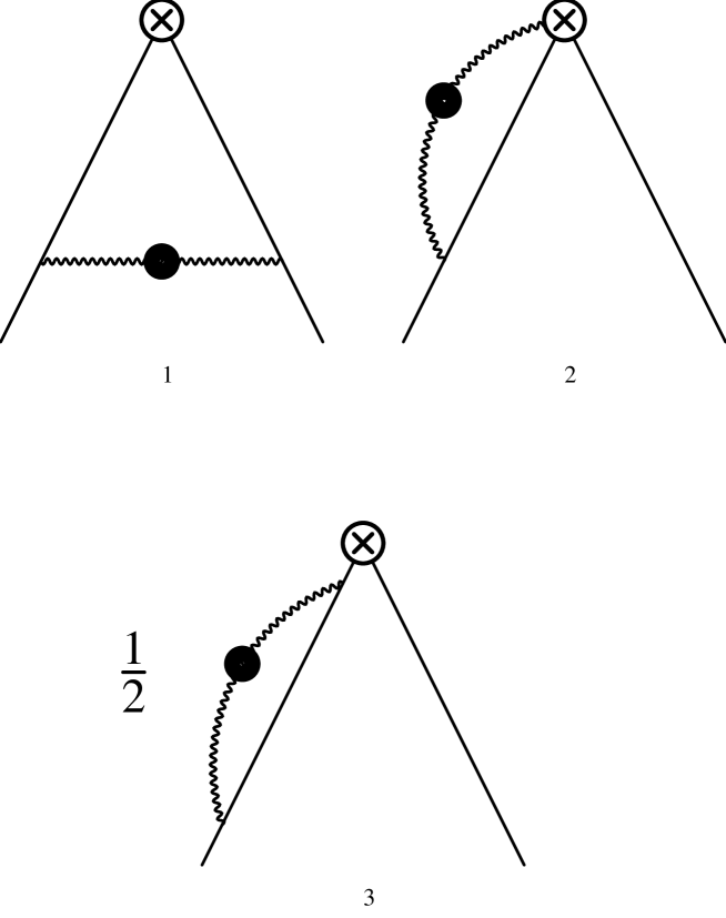
Figure 5: The diagrams that contribute to the evolution kernel in the leading order approximation. For diagrams (2) and (3), the mirrors conjugate diagrams have to be added.

The relevant diagrams are shown in fig.5 . This kernel, as in the one loop case, (12) becomes symmetric after multiplication by $(y\bar{y})^{\alpha}$:

$$(y\bar{y})^{\alpha}V_{\alpha}(x,y)\ =\ W(y,x)\ =\ W(x,y)\ .$$

This fact allows us to obtain the eigenfunctions and eigenvalue of the kernel $V_{\alpha}(x,y)$ .

$$\int^{1}_{0}V_{\alpha}(x,y)\bar{\varphi}_{n}(y,\mu^{2}) = -\gamma_{n}(\alpha_{s})\bar{\varphi}_{n}(x,\mu^{2})\ ,$$ (32)

$$\bar{\varphi}_{n}(x,\mu^{2}) = (x\bar{x})^{\alpha}\varphi_{n}(x,\mu^{2})A_{n}(\alpha_{s})\ ,{}$$ (33)

$$\varphi_{n}(x,\mu^{2}) = C^{1/2+\alpha}_{2n}(1-2x)\ ,$$ (34)

$$A_{n}(\alpha_{s}) = \frac{\Gamma(1+2\alpha)}{\Gamma(\alpha)\Gamma(1+\alpha)}\frac{(2n)!}{(2\alpha)_{2n}}\frac{(1+2\alpha+4n)}{\alpha+n}\ {},$$ (35)

$$\int^{1}_{0}\varphi_{n}\bar{\varphi}_{k}dx = \delta_{kn}\ ,$$ (36)

The eigenvalues $\gamma_{n}(\alpha_{s})$ read:

$$\gamma_{n}(\alpha_{s}) = \frac{\alpha_{s}}{4\pi}C_{F}\frac{\alpha^{2}\Gamma(2\alpha+2)}{3(1+\alpha)\ \Gamma(1+\alpha)^{3}\Gamma(2-\alpha)}\left\{1-\frac{\alpha(\alpha+1)}{(\alpha+2n)(\alpha+1+2n)}\right.$$ (37)

$$+ \left.\frac{2(1+\alpha)}{\alpha}\left[\psi(1+\alpha+2n)-\psi(1+\alpha)\right]\right\}.{}$$

Here, $\psi(z)$ is given by $\psi(z)=\frac{d}{dz}\ln\Gamma(z)$. Notice that, as in the one loop case, quark current conservation implies $\gamma_{0}(\alpha_{s})=0$. From (33) we see that in our case it is natural to expand the distribution function in $C_{2n}^{3/2+\alpha_{s}b_{0}}$ Gegenbauer polynomials:

$$\varphi(x,\mu^{2})\ =\ (x\bar{x})^{1+\alpha_{s}b_{0}}\sum^{\infty}_{n=0}b_{n}(\mu^{2})A_{n}(\alpha_{s})C^{3/2+\alpha_{s}b_{0}}_{2n}(1-2x)\ ,{}$$ (38)

compare with (13). Substituting (38) in the evolution equation (31) and using orthogonality of $\bar{\varphi}_{n}$ and $\varphi_{k}$, we obtain the following equation for the moments $b_{k}(\mu^{2})$:

$$\left[\mu^{2}\frac{\partial}{\partial\mu^{2}}-b_{0}\alpha_{s}^{2}\frac{\partial}{\partial\alpha_{s}}\right]b_{k}(\mu^{2})=-b_{k}(\mu^{2})\gamma_{k}(\alpha_{s})-\sum^{k}_{\ell=0}C_{k\ell}(\alpha_{s})b_{\ell}(\mu^{2})\ .{}$$ (39)

where we have introduced the mixing matrix $C_{k\ell}(\alpha_{s})$, which arises due to the fact that now the eigenfunctions depend on $\alpha_{s}(\mu^{2})$. Technical details can be found in Appendix B. In (39), $b_{0}$ is the first coefficient of the $\beta$ function, and should not be confused with the moment $b_{0}(\mu)$, where an explicit $\mu$ dependence is indicated. We obtain a triangular system of linear differential equations for the coefficients $b_{p}(\mu^{2}),\ p=0,1,\ldots,k$. Introducing the vector

$${\bf B}\ =\ \left(\begin{array}[]{l}b_{0}(\mu^{2})\\ b_{1}(\mu^{2})\\ \vdots\\ b_{k}(\mu^{2})\\ \vdots\end{array}\right){}$$ (40)

our equations can be written in the following matrix form:

$$\left[\mu^{2}\frac{\partial}{\partial\mu^{2}}-b_{0}\alpha_{s}^{2}\frac{\partial}{\partial\alpha_{s}}\right]{\bf B}(\mu^{2})\ =\ -(\hat{\gamma}_{D}+\hat{C}){\bf B}(\mu^{2})\ .{}$$ (41)

Here, $\hat{\gamma}_{D}$ is a diagonal matrix, built of the eigenvalues (37), and $\hat{C}$ is the triangular mixing matrix of (39). The first $N$ elements of (40) can be obtained exactly for arbitrary $N$. One first notices that (39) implies that $b_{0}(\mu^{2})$ is constant because $C_{00}=\gamma_{0}=0$ (due to conservation of the axial current). For $b_{1}(\mu^{2})$, (39) implies

$$\left[\mu^{2}{\partial\over\partial\mu^{2}}-b_{0}\alpha_{s}^{2}{\partial\over\partial\alpha_{s}}\right]b_{1}(\mu^{2})=-[\gamma_{1}(\alpha_{s})+C_{11}(\alpha_{s})]b_{1}(\mu^{2})-C_{10}(\alpha_{s})b_{0}(\mu^{2}),{}$$ (42)

which can be solved using well known techniques. This procedure can now be repeated for $b_{2}(\mu^{2})$, $b_{3}(\mu^{2})$, $\ldots$.

The general solution to (39) is given by

$${\bf B}(\mu^{2})\ =\ \hat{U}(\mu^{2},\mu^{2}_{0}){\bf B}(\mu^{2}_{0})$$ (43)

with the evolution matrix

$$\hat{U}(\mu^{2},\mu^{2}_{0}) = P_{a}\exp\left\{\int\limits^{a(\mu^{2})}_{a(\mu^{2}_{0})}\frac{da^{\prime}}{b_{0}{a^{\prime}}^{2}}[\hat{\gamma}(a^{\prime})+\hat{C}(a^{\prime})]\right\}$$ (44)

$$\hat{U}(\mu^{2}_{0},\mu^{2}_{0}) = \hat{1}\ .{}$$ (45)

It follows that

$$b_{k}(\mu^{2})\ =\ \sum^{k}_{k^{\prime}=0}\left\{\hat{U}(\mu^{2},\mu^{2}_{0})\right\}_{kk^{\prime}}b_{k^{\prime}}(\mu^{2}_{0}),$$ (46)

and we obtain the following expression for $\varphi(x,\mu^{2})$:

$$\varphi(x,\mu^{2})=(x\bar{x})^{1+\alpha_{s}b_{0}}\sum^{\infty}_{k=0}\left\{\hat{U}(\mu^{2},\mu^{2}_{0})\right\}_{kk^{\prime}}b_{k^{\prime}}(\mu^{2}_{0})A_{k}(\alpha_{s})C^{3/2+\alpha_{s}b_{0}}_{2k}(1-2x)\ ,$$ (47)

where we sum for $k^{\prime}\leq k$.

We have found numerically that the matrix elements of the nondiagonal part of the mixing matrix $\hat{C}$ are much smaller than the diagonal matrix elements of the sum $\hat{\gamma}+\hat{C}$ for all resonable values of $\mu^{2}$. We plot the matrix elements for $\mu^{2}=5$ GeV² in fig.6.a and fig.6.b. The diagonal elements are clearly bigger than the non diagonal ones. This happens for the whole range of relevant $\mu^{2}$.

6.a	6.b
6.c	6.d

Figure 6: In 6.a we show the nondiagonal elements $C_{k\ l}$ for $k=0,1,\cdots,15$, $l=0,1,2,\cdots,k-1$ and $\mu^{2}=5$ GeV². In 6.b we compare the nondiagonal elements, 6.a, with the diagonal ones, $\gamma_{m}+C_{mm},\ m\leq 15$. The effect of the nondiagonal terms on the evolution of $b_{1}(\mu^{2}),b_{2}(\mu^{2})$ is displayed for $(b_{0},b_{1},b_{2})(1$ GeV${}^{2})=(1,0,0)$ (6.c), and for $(b_{0},b_{1},b_{2})(1$ GeV${}^{2})=(1,1.7,1.6)$ (6.d).

We can therefore solve equation (41) by iterations with respect to the nondiagonal part $\hat{C}$. At leading order, neglecting the nondiagonal part of the mixing matrix, all coefficients $b_{k}(\mu^{2})$ renormalize multiplicatively, and the distribution function has the following form:

$$\varphi(x,\mu^{2}) = (x\bar{x})^{1+b_{0}\alpha_{s}}\sum^{\infty}_{k=0}b_{k}(\mu^{2})A_{k}(\alpha_{s})C^{3/2+\alpha_{s}b_{0}}_{2k}(1-2x)\ ,{}$$ (48)

$$b_{k}(\mu^{2}) = b_{k}(\mu_{0}^{2})\exp\left\{\int_{\alpha_{s}(\mu^{2}_{0})}^{\alpha_{s}(\mu^{2})}\frac{\gamma_{k}(x)+C_{kk}(x)}{b_{0}x^{2}}dx\right\},{}$$ (49)

where

$$C_{kk}(\alpha_{s})=(\alpha_{s}b_{0})^{2}\left\{\psi\left(\frac{1}{2}+\alpha+2k\right)-\psi\left(\alpha+\frac{1}{2}\right)\right\}.$$ (50)

4.2 Models for the distribution function

We have already mentioned that the distribution functions is not predicted by perturbative QCD. In this subsection we discuss some models for the distribution function. For any physical distribution function, the first coefficient $b_{0}(\mu^{2})$ of the expansion (48) is 1, as it follows from normalization

$$\int\limits^{1}_{0}\varphi(x,\mu^{2})dx\ =\ 1.$$ (51)

To extract the coefficients $b_{k}(\mu_{0}^{2})$ for $k>0$, some information about the low energy shape of the distribution function is needed. At present, some sum rule estimates are available. The second moment

$$\int_{0}^{1}(2x-1)^{2}\varphi(x,\mu^{2}_{0})dx=0.35\quad(\mu^{2}_{0}=1\ \rm{GeV}^{2}){}$$ (52)

has been estimated in [18, 19], and the following estimation for $\varphi(1/2)$ can be found in [19]:

$$\varphi(1/2,\mu^{2}_{0})=1.2\pm 0.3{}$$ (53)

For the second moment, the asymptotic distribution function predicts

$$\int_{0}^{1}\varphi_{as}(x)(2x-1)^{2}=0.2,{}$$ (54)

and for $x=1/2$, its prediction is $\varphi_{as}(1/2)=3/2$.

The estimation (52) would imply $b_{1}(\mu_{0}^{2})=1.1$ in the one loop expansion (13), and $b_{1}(\mu_{0}^{2})=1.7$ in the NNA expansion (48). The coefficient in the NNA expansion is $45\%$ bigger than the 1 loop coefficient. To be consistent with the central value of (53), we need at least the third coefficient of the expansion of the distribution functions, that is,

$$\varphi(x)=[x(1-x)]^{1+b_{0}\alpha_{s}}\left(A_{0}(\alpha_{s})+b_{1}A_{1}C_{2}^{3/2+b_{0}\alpha_{s}}(1-2x)+b_{2}A_{2}C_{4}^{3/2+b_{0}\alpha_{s}}(1-2x)\right){}$$ (55)

in the NNA approximation, and (55) with $\alpha_{s}=0$ in the one loop approximation. In (55), $A_{i}({\alpha_{s}})$ are given by (35). In the one loop expansion, (13),this implies $b_{2}(\mu_{0}^{2})=1.0$, and in the NNA expansion, (48) $b_{2}(\mu_{0}^{2})=1.6$. We have represented graphically both functions in fig.7. We agree with [19] that the higher harmonics remove the oscillations and make the function smoother.

Figure 7: Several distribution functions. Solid line: asymptotic distribution function. Dot-dashed line: one-loop distribution function obtained by combining sum rule results (52) and the prediction (53). Dashed line: NNA distribution function, (55) obtained as above. Here, $\mu_{0}^{2}=$ 1 GeV².

The evolution of the moments $b_{k}(\mu^{2})$ with $\mu^{2}$ is given by (39). It can be shown the in the limit $\mu\rightarrow\infty$, all $b_{i>0}(\mu^{2})$ tend to zero. This follows from the fact that at the one loop level the NNA approximation reduces to the exact one loop approximation. Then only the lowest momentum, $b_{0}(\mu^{2})$ will be relevant in the limit $\mu\rightarrow\infty$. This leads to the asymptotic wave function :

$$\varphi_{as}(x)=\lim_{\mu\rightarrow\infty}\frac{\Gamma(4+2b_{0}\alpha_{s})}{\Gamma^{2}(2+b_{0}\alpha_{s})}[x(1-x)]^{1+b_{0}\alpha_{s}}=6x(1-x).{}$$ (56)

It is interesting to see the difference between the asymptotic shape and the lowest order NNA harmonic, which depends on $\alpha_{s}$. In fig.8 we can see that the lowest NNA harmonic is a little bit narrower than $\varphi_{as}(x)$.

Figure 8: Solid line: asymptotic distribution function. Dashed line: Asymptotic NNA distribution function (56) for $Q^{2}=10{\rm GeV}^{2}$. Dot-dashed line: the same for $Q^{2}=1{\rm GeV}^{2}$.

The effect of the nondiagonal terms $C_{k\ l}$ on the evolution of the coefficients of the two models presented in this subsection has been displayed in fig.(6).c and fig.(6).d. In fig.(6).c we have solved the differential equation (39) exactly for the initial condition corresponding to (56), that is, $b_{0}(1$ GeV${}^{2})$ = 1, $b_{i>0}(1$ GeV${}^{2})$ = 0. Here, the diagonal solution (49) predicts $b_{1}(\mu^{2})=b_{2}(\mu^{2})=0$, while the exact solution is negative, and quite small. In fig.(6).d we have used the initial conditions the nondiagonal elements $C_{k\ l}$ for the initial condition $b_{0}(1$ GeV${}^{2})$ = 1, $b_{1}(1$ GeV${}^{2})$ = 1.7 and $b_{2}(1$ GeV${}^{2})$ = 1.6, which is obtained by combining a sum rule prediction for the first moment, [19, 18], and a prediction for $\varphi(1/2)$, [19]. The moments $b_{k}(\mu)^{2}$ are the matrix elements of the operators

$$\bar{d}\gamma_{5}(\hat{n})(n\partial)^{2n}_{+}C^{3/2+b_{0}\alpha_{s}}_{2n}(nD_{-}/(n\partial)_{+})u.{}$$ (57)

which renormalize multiplicatively. It might be convenient to redefine the one loop operators (15) in order to extract from the diagonal part all the main corrections.

4.3 Conformal symmetry constraints

We will now make some comments on the diagonalization of the evolution kernel and its eigenfunctions based on conformal invariance arguments. We start with the observation that at the one loop level we have conformal invariance, which gets broken when we go to higher orders. Conformal symmetry is broken by the introduction of the renormalization scale $\mu$, and due to renormalization scheme effects [16]. The breaking due to the renormalization of the coupling are, to our accuracy, proportional to the first coefficient of the $\beta-$ function, while those due renormalization scheme effects are $1/N_{f}^{2}$ suppressed, and therefore lie beyond our accuracy. Despite the fact that conformal symmetry is broken, it still allows us to diagonalize the evolution kernel. This is equivalent to the diagonalization of the anomalous dimension matrix. The fact that the anomalous dimension matrix can be diagonalized at any order in perturbation theory follows from conformal invariance at the one loop level, where (16) is implied. In general, the eigenvalues will be given by a series in $\alpha_{s}$. Since there are no two eigenvalues with the same lowest order coefficient, (16), all eigenvalues are different, and we can therefore diagonalize the anomalous dimension matrix.

Consider now the renormalization group equations for the operators defined in (15) for higher orders in perturbation theory:

$$\mu^{2}\frac{d}{d\mu^{2}}O_{R}=\hat{\gamma}O_{R},{}$$ (58)

where $O_{R}$ are the renormalized operators, and $\hat{\gamma}$ is the anomalous dimension matrix, which is only diagonal at the one loop level. Since it can be diagonalized, there is a matrix $\hat{U}(\alpha_{s})$ such that

$$\hat{\gamma}(\alpha_{s})=\hat{U}^{-1}(\alpha_{s})\hat{\gamma}_{D}(\alpha_{s})\hat{U}(\alpha_{s}){}$$ (59)

where $\hat{\gamma}_{D}$ is a diagonal matrix. Substituting this representation in (58) and redefining the operators

$$\tilde{O}_{R}(\alpha_{s})=\hat{U}(\alpha_{s})O_{R}$$ (60)

it is easy to obtain the following equation for the new operators $\tilde{O}_{R}$:

$$\mu^{2}\frac{d}{d\mu^{2}}\tilde{O}_{R}=\left\{\hat{\gamma}_{D}(\alpha_{s})-\hat{U}(\alpha_{s})\left(\mu^{2}\frac{d}{d\mu^{2}}\hat{U}^{-1}(\alpha_{s})\right)\right\}\tilde{O}_{R}{}$$ (61)

In the rhs, the coefficient in front of $\tilde{O}_{R}$ is its anomalous dimension. It is clear that to our accuracy, we can associate the diagonalization of the matrix $\hat{\gamma}$ with the diagonalization of the kernel $V_{\alpha}(x,y)$. Then, the nondiagonal part, $\hat{U}(\alpha_{s})\left(\mu^{2}\frac{d}{d\mu^{2}}\hat{U}(\alpha_{s})\right)$ is the mixing matrix $\hat{C}(\alpha_{s})$ and the operator $\tilde{O}_{R}(\alpha_{s})$ is given in (57).

In $D=4-2\epsilon$ dimensions, the $\beta$-function has the following form:

$$\beta(\epsilon,\alpha_{s})=-\epsilon\alpha_{s}-b_{0}\alpha_{s}^{2}+\cdots{}$$ (62)

and there is a critical value for the coupling (or fixed point ) $\alpha_{s}^{\ast}$ such that

$$\beta(\epsilon,\alpha_{s}^{\ast})=0{}$$ (63)

To first order in the large $N_{f}$ expansion, (62) implies

$$\alpha_{s}^{\ast}=\frac{3\epsilon}{2N_{f}}(4\pi)+O(1/N_{f}^{2})$$ (64)

Consider now equation (61) at the critical point. Than nondiagonal part vanishes:

$$\hat{U}(\alpha_{s})\left(\mu^{2}\frac{d}{d\mu^{2}}\hat{U}^{-1}(\alpha_{s})\right)|_{\alpha_{s}=\alpha_{s}^{\ast}}=\beta(\epsilon,\alpha_{s})\hat{U}(\alpha_{s})\left(\frac{d}{d\alpha_{s}}\hat{U}^{-1}(\alpha_{s})\right)|_{\alpha_{s}=\alpha_{s}^{\ast}}=0,$$ (65)

due to (63), and $\tilde{O}_{R}(\alpha_{s}^{\ast})$ has a diagonal anomalous dimension matrix $\hat{\gamma}_{D}(\alpha_{s}^{\ast})$ at the critical point. For the operators (57), taking into account that we have to perform the substitution $2/3N_{f}\rightarrow 2/3N_{f}-11/3N_{c}$ “by hand”, and then $\alpha_{s}^{\ast}=-\epsilon/b_{0}$, we obtain

$$\tilde{O}_{R}(\alpha_{s}^{\ast})=\bar{d}\gamma_{5}(\hat{n})(n\partial)^{2n}_{+}C^{3/2+b_{0}\alpha_{s}^{\ast}}_{2n}(nD_{-}/(n\partial)_{+})u=\bar{d}\gamma_{5}(\hat{n})(n\partial)^{2n}_{+}C^{3/2-\epsilon}_{2n}(nD_{-}/(n\partial)_{+})u{}$$ (66)

The last equation shows that the basis (57) is conformal at the critical point because the classical conformal composite operator, built of two fermion fields $\bar{\psi},\ \psi$ is given by [23]:

$$\bar{\psi}\gamma_{5}(\hat{n})(n\partial)^{2n}_{+}C^{d_{\psi}}_{n}(nD_{-}/(n\partial)_{+})\psi\ ,$$ (67)

where $d_{\psi}$ is the canonical dimension of the fermion field. In $D=4-2\epsilon$ dimensions, $d_{\psi}=3/2-\epsilon$. We have checked by explicit calculation that at the critical point, $\alpha_{s}^{\ast}=\frac{3\epsilon}{2N_{f}}(4\pi)$, and to leading order in the large $N_{f}$ expansion, the operators (66) have a diagonal anomalous dimension matrix $\gamma_{D}(\alpha_{s}^{\ast})$.

We conclude that conformal symmetry operators at the critical point and the operators $\tilde{O}_{R}(\alpha_{s})$ that diagonalize the evolution kernel at leading order in $1/N_{f}$ are related: The operators $\tilde{O}_{R}(\alpha_{s})$ can be obtained from the the conformal ones by the replacement $(-\epsilon)\rightarrow b_{0}\alpha_{s}$. We should notice that this result is rigorous at leading order in the $1/N_{f}$ expansion. However, we follow the prescription of NNA, and replace $2/3N_{f}\rightarrow 2/3N_{f}-11/3N_{c}$. It seems reasonable to assume that the nondiagonal part of the anomalous dimension matrix induced by this will be small.

5 The form factor

Below we calculate the form factor (5) for $\omega=1$. In this case, (5) reads:

$$F_{\pi\gamma}(Q^{2})\ =\frac{N}{Q^{2}}\int^{1}_{0}\left(C_{0}(x)+C_{1}(x,Q^{2})+C_{0}(1-x)+C_{1}(1-x,Q^{2})\right)\varphi(x,Q^{2})dx\ ,\ {}$$ (68)

where for simplicity we set $\mu^{2}=Q^{2}$. $C_{0}(x)$,  $C_{1}(x,Q^{2})$ can be obtained from (25) and (26), and $\varphi(x,Q^{2})$ is given by (48).

We have already seen that the coefficient function (26) is ill defined in the limit $x\rightarrow 0$ and $x\rightarrow 1$ because we expand in $\Lambda^{2}/(xQ^{2})$ or $\Lambda^{2}/((1-x)Q^{2})$. This induces uncertainties which are related to the nonperturbative structure of QCD in the infrared region and induce power corrections to the form factor. In addition to the power contributions from the $IR$-renormalon ambiguity, the form factor can get qualitatively different power corrections from the regions $x\rightarrow 0$ and $x\rightarrow 1$. These new power corrections can be related to new contributions which correspond to the new regimes, see fig.1.2 and 1.3. As discussed above, the leading contributions of these regimes are of order $1/Q^{4}$ and become essential in the limit $\omega\rightarrow 1$. To perform a phenomenological analysis of the power uncertainty related to the regions $x\rightarrow 0$ and $x\rightarrow 1$, we first observe that the all the ambiguities come from the Borel integral of $C_{1}(x,Q^{2})$, see (26), and interchange the order of integration, that is, integrate first over $x$, and then over the Borel parameter $u$. Using the property $\varphi(x)=\varphi(1-x)$ we rewrite (68) as:

$$F_{\pi\gamma}(Q^{2})\ =2\frac{N}{Q^{2}}\int^{1}_{0}\left(C_{0}(x)+C_{1}(x,Q^{2})\right)\varphi(x,Q^{2})dx\ .$$ (69)

The complete integration over $x$ can be done analytically. In principle, it is only necessary to interchange the order of integration in the Borel integral in (26), because the other integral is well defined. We obtained an expression for the form factor in which all ambiguities are related to the poles of the function in the Borel integral. The integration over $x$ yields (below $\alpha\equiv 1+b_{0}\alpha_{s}$):

$$F_{\pi\gamma}(Q^{2})\ =\ {N\over Q^{2}}\sum^{\infty}_{k=0}\frac{(2k)!}{(2\alpha)_{2k}}\frac{(1+2\alpha+4k)}{(\alpha+k)}b_{k}(Q^{2})\left\{1-{C_{F}\over 4\pi b_{0}}M_{k}(\alpha_{s})\right\}\ ,{}$$ (70)

$$\ M_{k}(\alpha_{s})\ =\ p.v.\int\limits^{\infty}_{0}e^{-u/b_{0}\alpha_{s}}\frac{du}{u}\left\{e^{u(C-ln2)}\frac{2\Gamma(\alpha-u)}{(1-u)(2-u)\Gamma(\alpha)}\theta_{k}(\alpha_{s},u)-\theta_{k}(\alpha_{s},0)\right\}{}$$

$$+\ \ \int^{\alpha}_{1}\ \frac{d\lambda}{1-\lambda}\{\rho_{k}(\alpha_{s},\lambda)-\rho_{k}(\alpha_{s},1)\}\ ,$$ (71)

$$\theta_{k}(\alpha_{s},u)=3\frac{(1+u)_{2k}}{(2k)!}\ \frac{\Gamma(1+2\alpha+2k)}{\Gamma(1+2\alpha-u+2k)}+\frac{(1+u)_{2k}}{(2k)!}\frac{(2-u)(1+u)(\alpha-u)}{(1+u+2k)}$$

$$\times\frac{\Gamma(1+2\alpha+2k)}{\Gamma(2+2\alpha-u+2k)}{}_{3}F_{2}\left[\begin{array}[]{l}1,1,\ 1+\alpha+2k\\ 2+u+2k,2+2\alpha-u+2k\end{array}|1\right]$$ (74)

$$-\ \ \frac{2\Gamma(1+2\alpha+2k)}{\Gamma(1+2\alpha-u+2k)}\sum^{2k}_{\ell=0}\ \frac{(1+u)_{\ell}}{(1+u+\ell)\ell!}\ _{3}F_{2}\ \left[\begin{array}[]{l}1,1,\ 1+\alpha+2k\\ 2+u+\ell,1+2\alpha-u+2k\end{array}|1\right]\ .$$ (77)

$$\rho_{k}(\alpha_{s},\lambda) = \frac{\Gamma(2+2\lambda)}{3\Gamma(2-\lambda)\Gamma^{3}(1+\lambda)}\left\{\frac{2+2\lambda-\lambda^{2}}{1+\lambda}+\right.$$ (80)

$$+ \frac{\alpha\lambda^{2}}{(\lambda+2k)(1+2\alpha+2k)}\ _{3}F_{2}\left[\begin{array}[]{l}1,\lambda,\ 1+\alpha+2k\\ 1+\lambda+2k,2+2\alpha+2k\end{array}|1\right]$$

$$- \left.\sum^{2k}_{\ell=0}\ \frac{\lambda}{\lambda+\ell}\ _{3}F_{2}\left[\begin{array}[]{l}1,\lambda,\ 1+\alpha+2k\\ 1+\lambda+\ell,1+2\alpha+2k\end{array}|1\right]\right\}\ .$$ (83)

Where ${}_{3}F_{2}[\cdots|1]$ is the standard hypergeometric function (3,2), $(z)_{n}=\frac{\Gamma(z+n)}{\Gamma(z)}$ is the Pochhammer symbol, and $C_{F}=(N_{c}^{2}-1)/(2N_{c})$. We have absorbed all the singularities in the factor ${\Gamma(1+b_{0}\alpha_{s}-u)}/[{\Gamma(1+b_{0}\alpha_{s})(1-u)(2-u)}]$ of the Borel integral in (5). There are two renormalon poles at $u=1$ and $u=2$, and an infinite number of new “small-$x$” poles at $u=1+b_{0}\alpha_{s}+m,\ m=0,1,\cdots$. We will integrate the poles following the principal value prescription. The final result will be prescription dependent, but this dependence is known to be power suppressed.

To estimate the size of the higher power corrections, we will follow the recipe of Section 2: A pole at $u=u_{0}$ induces a power correction of order $(\Lambda^{2}/Q^{2})^{u_{0}}$. The entire power correction to the form factor can written in the following way:

$$\Delta F_{\pi\gamma}(Q^{2}) = \pm\frac{N}{Q^{2}}\left(N_{1}\Delta_{2}(\alpha_{s})\left(\frac{\Lambda}{Q}\right)^{2}+K_{1}\delta_{2}(\alpha_{s})\left(\frac{\Lambda^{2}}{Q^{2}}\right)^{1+b_{0}\alpha_{s}}+\cdots\right)=$$ (84)

$$\pm \frac{N}{Q^{2}}\left(\{N_{2}\Delta_{2}(\alpha_{s})+K_{2}\delta_{2}(\alpha_{s})e^{-1}\}\left(\frac{\Lambda}{Q}\right)^{2}+\cdots\right)\ .{}$$

In the last identity we have used the one-loop expression for the running coupling. By the dots, we denote the contributions of the higher poles, $u=2,\ \mbox{and}\ u=1+b_{0}\alpha_{s}+m,\ m=1,2,\cdots$. The contribution $N_{1}\Delta_{2}(\alpha_{s})$ is related to the first renormalon pole, $u=1$. The function $\Delta_{2}(\alpha_{s})$ is build of the residues of the integrand of the Borel integral, and can be calculated, and $N_{1}$ is an unknown number of order one. The second contribution is related to the “small-$x$” poles. Its structure is the same, $K_{1}$ is an unknown constant and $\delta_{1}(\alpha_{s})$ a calculable function. We finally obtain:

$$F_{\pi\gamma}(Q^{2})\ = \frac{N}{Q^{2}}\left(\sum^{\infty}_{k=0}\frac{(2k)!}{(2\alpha)_{2k}}\frac{(1+2\alpha+4k)}{(\alpha+k)}b_{k}(Q^{2})\left\{1-C_{F}/b_{0}M_{k}(\alpha)\right\}\right.$$ (85)

$$\pm \left.\{N_{2}\Delta_{2}(\alpha_{s})+K_{2}\delta_{2}(\alpha_{s})e^{-1}\}\left(\frac{\Lambda}{Q}\right)^{2}+\cdots\right).{}$$

Here, we are neglecting $1/Q^{4}$ and higher power contributions. To make a numerical estimation, we only take, for simplicity, the first term of the expansion of the distribution function (56)

$$\varphi(x,Q^{2})=\frac{\Gamma(4+2b_{0}\alpha_{s})}{\Gamma^{2}(2+b_{0}\alpha_{s})}[x(1-x)]^{1+b_{0}\alpha_{s}},\ \alpha_{s}\equiv\alpha_{s}(Q^{2}).{}$$ (86)

As discussed above, this approximation is very close to the asymptotic form. Then, in the expression for the form factor (70), we have to keep only the first term. This gives:

$$F_{\pi\gamma}(Q^{2})\ =\frac{N}{Q^{2}}\frac{(1+2\alpha)}{\alpha}\left\{1-{C_{F}\over 4\pi b_{0}}M_{0}(\alpha_{s})\right\}\pm\mbox{power corrections}{}$$ (87)

$$\ M_{0}(\alpha_{s})\ =\ p.v.\int\limits^{\infty}_{0}e^{-u/b_{0}\alpha_{s}}\frac{du}{u}\left\{e^{u(C-ln2)}\frac{\Gamma(\alpha-u)}{\Gamma(\alpha)}\frac{2\theta_{0}(\alpha_{s},u)}{(1-u)(2-u)}-\theta_{0}(\alpha_{s},0)\right\}$$

$$+\ \ \int^{\alpha}_{1}\ \frac{d\lambda}{1-\lambda}\{\rho_{0}(\alpha_{s},\lambda)-\rho_{0}(\alpha_{s},1)\}\ ,$$ (88)

(89)

$$\theta_{0}(\alpha_{s},u)=\Gamma(1+2\alpha)\left\{\frac{3}{\Gamma(1+2\alpha-u)}+\frac{(2-u)(\alpha-u)}{\Gamma(2+2\alpha-u)}{}_{3}F_{2}\left[\begin{array}[]{l}1,1,\ 1+\alpha\\ 2+u,2+2\alpha-u\end{array}|1\right]\right.$$ (92)

$$\left.-\ \ \frac{2}{\Gamma(1+2\alpha-u)(1+u)}{}_{3}F_{2}\ \left[\begin{array}[]{l}1,1,\ 1+\alpha\\ 2+u,1+2\alpha-u\end{array}|1\right]\ \right\}$$ (95)

$$\rho_{0}(\alpha_{s},\lambda) = \frac{\Gamma(2+2\lambda)}{3\Gamma(2-\lambda)\Gamma^{3}(1+\lambda)}\left\{\frac{2+2\lambda-\lambda^{2}}{1+\lambda}+\frac{\alpha\lambda}{(1+2\alpha)}\right.$$

$$\times {}_{3}F_{2}\left[\begin{array}[]{l}1,\lambda,\ 1+\alpha\\ 1+\lambda,2+2\alpha\end{array}|1\right]\left.-{}_{3}F_{2}\left[\begin{array}[]{l}1,\lambda,\ 1+\alpha\\ 1+\lambda,1+2\alpha\end{array}|1\right]\right\}\ .$$

At leading order, we obtain

$$F_{\pi\gamma}^{LO}(Q^{2})\ =3\frac{N}{Q^{2}}{}$$ (97)

To obtain the next-to-leading, or 1-loop result, we expand (86) in series of $\alpha_{s}$:

$$\varphi(x,Q^{2})=6x(1-x)\{1+b_{0}\alpha_{s}(Q^{2})[5/3+\ln(x(1-x))]\}+O(\alpha_{s}^{2}).$$ (98)

The coefficient function (26) in the one loop limit gives the well known one-loop formula (6), and to next-to-leading order in $\alpha_{s}$, we obtain:

$$F_{\pi\gamma}^{NLO}(Q^{2})\ = \frac{N}{Q^{2}}\left\{3+6\alpha_{s}b_{0}\int_{0}^{1}(1-x)\bigg{[}{5\over 3}+\ln[x(1-x)]\bigg{]}dx\right.$$ (99)

$$+ \left.C_{F}\frac{\alpha_{s}}{4\pi}\int_{0}^{1}(1-x)\bigg{[}\ln 2(3+2\ln x)+\ln^{2}(x)-\ln(1-x)-9\bigg{]}dx\right\}=$$

$$= 3\frac{N}{Q^{2}}\left(1-\frac{1}{3}b_{0}\alpha_{s}-5C_{F}{\alpha_{s}\over 4\pi}\right){}$$

The contribution of higher order radiative corrections in the NNA approximation is given by (87). Numerical results are presented in fig.9. For $\alpha_{s}(Q^{2})$, we use $\alpha_{s}(m_{\tau}^{2})=0.32,\ N_{f}=4$, and take into account that in the $\overline{MS}$-scheme $C=5/3$. We see that the one loop correction decreases the leading order result by $20\%$. Higher order contributions, together with the one-loop correction, decrease the leading order by $30\%$. This estimation is in agreement with the estimations for radiative corrections suggested in [10].

Figure 9: The form factor $F_{\pi\gamma}$. The constant line $(Q^{2}/N)F_{\pi\gamma}=3$ corresponds to the lowest order prediction, (97). The next to leading result, (99) is plotted with long dashes, while the dots represent the NNA prediction, (87), and the two solid lines represent the uncertainties in the resummation. The dot-dashed line is the semisum of the NNA result and the next to leading prediction, and we expect the real result not to lie far away from it.

The difference between our distribution function and the asymptotic one is very small and, for example, a discrimination in the description of the NLO correction to the form factor will be very difficult. Let us remind that in [10] it has been assumed that the corrections due to the evolution of the distribution function are so small that they can be neglected.

To obtain the power corrections, we set the unknown constants $K_{2}$ and $N_{2}$ in (84) equal to 1. We find that in our approach the power corrections give an ambiguity of order $10-2\%$ for $2{\rm GeV}^{2}<Q^{2}<10{\rm GeV}^{2}$. Below we give some numerical results in the following form:

$$N^{-1}Q^{2}F_{\pi\gamma}(Q^{2})=F_{\pi\gamma}^{NLO}(Q^{2})-(\mbox{number1})\pm(\mbox{number2}),$$ (100)

where “number1” is the contribution of the higher order radiative corrections in the NNA approximation, and “number2” is the power correction (ambiguity in the summation of the perturbation series).

$Q^{2}$ $(\rm{GeV})^{2}$	$N^{-1}Q^{2}F_{\pi\gamma}$
2	2.20-0.36$\pm$0.19
3	2.27-0.36$\pm$0.14
4	2.31-0.35$\pm$0.12
5	2.34-0.34$\pm$0.10
6	2.36-0.33$\pm$0.08
7	2.38-0.32$\pm$0.07
8	2.40-0.31$\pm$0.07
9	2.41-0.30$\pm$0.06
10	2.42-0.29$\pm$0.06

Table 1: Some numerical results for the form factor

For the last number, see (84), we set $N_{2}=N_{4}=K_{2}=K_{4}=1$ (in this calculation we take into account small terms of order $(\Lambda/Q)^{4}$). Such choice fixes the relative sign of renormalon and small x ambiguities which is also unknown. In Fig.10 we have plotted the separate contribution of the first 4 poles to the ambiguity. It is interesting to notice that the first renormalon pole ambiguity, due to the $u=1$ singularity, and the first small $x$ ambiguity, due to the $u=1+\alpha_{s}b_{0}$ have different sign, which results in a partial cancelation of the ambiguity. This cancelation suggests that the contributions of the matrix elements of the higher twist operators will partially cancel with contributions coming from photon emission at large distances.

Other choice, such as for example $N_{2}=-K_{2}=1$, which would lead to a bigger uncertainty ($40\%$ at $Q^{2}=2$ GeV² and $10\%$ at $Q^{2}=10$ GeV² ), could also have been adopted. At present we have no rigorous arguments to choose the relative sign. Any of these definitions can only provide us with an estimation for the uncertainty.

Figure 10: The separate contribution of each pole to the uncertainty.

As a rule, NNA resummations give an exceeding estimation for the higher order contributions, see for example [8], and the real curve for the form factor might lie a little above the one suggested by the NNA approximation in fig.9 but below the one loop approximation. We have plotted an estimation for the real curve in the fig.9 with long dashed (short gaps) line.

To understand better the shape of the distribution function, we have to consider at least the model of the distribution function (55) which was obtained from the consideration of the sum rule constraints. This is work in progress, [25].

6 Conclusions

We have obtained the photon $\pi^{0}$-meson form factor at leading order in ‘naive nonabelianization’ (NNA). We have computed the coefficient function and the evolution kernel that governs the evolution of the distribution function, in the NNA approximation.

To evaluate the coefficient function and the evolution kernel, all leading contributions in $(-b_{0}\alpha_{s})^{n}$ have to be computed and resummed. For the coefficient function, Borel integral techniques have been used to perform the summation. Due to the presence of (IR) renormalons in the integrand, a prescription to perform the integration has to be chosen. We have used the principal value prescription. The assumption of ultraviolet dominance of higher twist matrix element has allowed us to obtain an estimation of higher twist contributions (ambiguity in the resummation). We have found that when one of the photons is on shell, the coefficient function has new singularities. These new singularities are caused by new IR regions, that appear when one of the quarks that build the pion carries almost no momentum. The power correction induced by these new singularities have been taken into account.

We have found that conformal constraints allow to find a basis of operators that diagonalizes the evolution kernel in the NNA approximation, but the anomalous dimension matrix is nondiagonal. The nondiagonal terms of the anomalous dimension matrix have been found to be much smaller than the diagonal elements and we neglected by them. We have obtained an expansion of the distribution function in series of Gegenbauer polynomials with multiplicatively renormalized moments. This form is very convenient to analyze the effects of radiative corrections. Radiative corrections make the shape of the first term in the expansion of the distribution function a little bit narrower as compared to the one loop term but, we find that this effect is small. We have calculated the convolution of the coefficient function and the distribution function, and obtained the form factor as a sum with unknown nonperturbative coefficients, which depend on the shape of the wave function in the low energy region. In our numerical analysis, we only keep the first term in the expansion of the distribution function. We obtained that the radiative correction decrease the leading order by $30\%$. This is consistent with the estimation for the radiative correction by [10]. The value of the power suppressed corrections (ambiguity in the resummation) depends on the relative sign of renormalon and small x ambiguities. It will be smaller for the case when they have different sign and predict the uncertainty for the value of the form factor from $10\%$ at $Q^{2}=2{\rm GeV}^{2}$ to $2\%$ at $Q^{2}=10{\rm GeV}^{2}$. The different sign of the ambiguities implies that nonperturbative effects coming from the matrix elements of the higher twist operator and soft photon emission is partially cancelled. In case of the similar sign the uncertainty for the value of the form factor is bigger: from $40\%$ at $Q^{2}=2{\rm GeV}^{2}$ to $10\%$ at $Q^{2}=10{\rm GeV}^{2}$. Clearly, an investigation of the influence of the higher harmonics in the expansion of the distribution function is needed. This will allow us to understand better the structure of the distribution function in the low energy region.

Acknowledgments. We are grateful to V. Braun., who initiated this work, for the numerous discussions and critical reading of this paper. We also thank S. Peris for the critical reading of the manuscript, and A. Radyushkin and D. Müller for discussions. N. K. thanks NORDITA for hospitality where the part of this work has been done. P. G. acknowledges gratefully a grant from the Spanish ministry for education and culture (MEC).

Appendix A

All calculations have been performed in dimensional regularization in $D=4-2\epsilon$ dimensions. For the gluon propagator, we use the Landau gauge. To solve the $\gamma_{5}$ - problem, we have followed the prescription of [3], where an anticommuting $\gamma_{5}$ was only used in the box diagram. The unrenormalized contribution of each diagram $D_{i}$ to the coefficient function can be represented in the following way:

$$D_{i} = -\frac{C_{F}}{4\pi}\sum^{\infty}_{n=0}\frac{1}{(1+n)\epsilon^{(n+1)}}\alpha_{s}^{1+n}(\mu^{2})(-\beta_{0}^{f})^{n}E_{i}[(n+1)\epsilon,\epsilon]\ ,{}$$ (A.1)

$$E_{i}[u,\epsilon] = \left(4\pi\frac{\mu^{2}}{Q^{2}}\right)^{u}\left(\frac{\Gamma(4-2\epsilon)}{6\Gamma(1+\epsilon)\Gamma^{2}(2-\epsilon)}\right)^{1-\frac{u}{\epsilon}}\frac{\Gamma(1-\epsilon)\Gamma(1+u)\Gamma(1-u)}{\Gamma(2-\epsilon+u)\Gamma(2-\epsilon-u)}R_{i}(\epsilon,u|x,\omega)\ ,$$

where $n$ is the number of fermion bubbles in the gluon propagator, $Q^{2}=-(q_{1}-q_{2})^{2}/4>0,\ \beta_{0}^{f}\ =\ \frac{2}{3}N_{f}/4\pi$ is the fermion part of the full $\beta_{0}=-b_{0}$, and only the factor $R_{i}(\epsilon,\Delta,x,\omega)$ is different for different diagrams. We will refer to the contribution of the $g_{\mu\nu}$ term in the gluon propagator as the “gauge invariant” contribution, and to the contribution from the $k_{\mu}k_{\nu}/k^{2}$ part as the “gauge dependent” contribution. The total contribution of the “gauge dependent” cancels, and we will in what follows only deal with the “gauge invariant” ones. In what follows, the notation

$$\alpha=1-\epsilon,\quad F(z)\equiv{}_{2}F_{1}(1,\alpha;1+\alpha+u|z)$$ (A.2)

where ${}_{2}F_{1}$ is the hypergeometric function (2,1), will be understood.

The contribution of the crossed diagram of $R$ will be denoted by $\bar{R}$, $C_{0}(x,\omega)$ denotes the Born contribution, see (19)). The diagrams are numbered according to fig.2:

$$R_{1}+\bar{R}_{1} = C_{0}^{1+u}(x,\omega)\frac{2\alpha^{2}(\alpha+u)}{1+\alpha-u}+\{x\leftrightarrow 1-x\}\ ,$$ (A.3)

$$R_{2}+\bar{R}_{3} = C_{0}^{1+u}(x,\omega)\left\{2(1-\alpha)(\alpha+u)+\frac{2\alpha(\alpha+u)}{1+\alpha-u}\right.$$

$$+ \left.\left(\frac{2\alpha u(\alpha-u)}{1+\alpha-u}-2(\alpha+u)\right)F\left(\frac{2\omega(1-x)}{1+\omega}\right)\right\}+\{x\leftrightarrow 1-x\}\ ,$$

$$R_{3}+\bar{R}_{2} = C_{0}^{1+u}(x,\omega)\left\{2(1-\alpha)(\alpha+u)+\frac{2\alpha(\alpha+u)}{1+\alpha-u}\right.$$

$$+ \left.\left(\frac{2\alpha u(\alpha-u)}{1+\alpha-u}-2(\alpha+u)\right)F\left(\frac{-2\omega x}{1-\omega}\right)\right\}+\{x\leftrightarrow 1-x\}\ ,$$

$$R_{4}+\bar{R}_{4} = C_{0}^{1+u}(x,\omega)\frac{\alpha(\alpha+u)}{C_{0}(x,\omega)\omega}\left\{F\left(\frac{2\omega(1-x)}{1+\omega}\right)-F\left(\frac{-2\omega x}{1-\omega}\right)\right\}+\{x\leftrightarrow 1-x\}\ .$$

From here, the subdivergences and the overall divergence have to be subtracted. In [26] a technique to perform this in the $MS$ scheme was developed. We will now extend their method to arbitrary schemes. First, one observes that a general diagram with $n$ fermion blob insertions into the gluon propagator can be expressed as (A.1):

$$D^{(n)}=(-1)^{n+1}C_{F}{\alpha_{s}\over 4\pi}{(\alpha_{s}\beta_{0}^{f})^{n}\over(n+1)\epsilon^{n+1}}E([n+1]\epsilon,\epsilon){}$$ (A.4)

where $E([n+1]\epsilon,\epsilon)$ is a continuous function for $\epsilon=0$. To subtract the subdivergences of the fermion bubbles, we also have to consider diagrams where at least one of the fermion bubbles is replaced by a counterterm:

$$-C_{F}{\alpha_{s}\over 4\pi}\sum_{k=0}^{n}{n\choose k}{(-\alpha_{s}\beta_{0}^{f})^{n-k}\over(n+1-k)\epsilon^{n+1-k}}E([n+1-k]\epsilon,\epsilon)\left({\alpha_{s}\beta_{0}^{f}e^{\Omega\epsilon}\over\epsilon}\right)^{k}{}$$ (A.5)

In (A.5), we have ($\ {}^{k}_{n}$) diagrams (permutations) containing $n-k$ fermion bubbles, (A.4) and $k$ counterterms. The subdivergences are cancelled by summing $k$ from 0 to $n$. In the $MS$ scheme, only the poles in $\epsilon$ are subtracted, and $\Omega_{MS}=0$, but in other schemes also finite parts are subtracted, and in what follows, we keep $\Omega\neq 0$. The structure of (A.5) suggests to define

$$E([n+1]\epsilon,\epsilon)=e^{(n+1)\Omega\epsilon}E_{\Omega}([n+1]\epsilon,\epsilon)$$ (A.6)

In terms of $E_{\Omega}$, (A.5) reads

$$-e^{(n+1)\Omega\epsilon}C_{F}{\alpha_{s}\over 4\pi}\sum_{k=0}^{n}{n\choose k}{(-\alpha_{s}\beta_{0}^{f})^{n-k}\over(n+1-k)\epsilon^{n+1-k}}E_{\Omega}([n+1-k]\epsilon,\epsilon)\left({\alpha_{s}\beta_{0}^{f}\over\epsilon}\right)^{k}{}$$ (A.7)

Now, $E([n+1]\epsilon,\epsilon)$ is expanded in the following way:

$$E_{\Omega}([n+1]\epsilon,\epsilon)=\sum_{j=0}^{\infty}\tilde{E}_{j}(\epsilon)([n+1]\epsilon)^{j},\qquad\tilde{E}_{0}(\epsilon)\equiv g(\epsilon)=\sum_{i=0}^{\infty}g_{i}\epsilon^{i}{}$$ (A.8)

We now use (A.8) to expand $E_{\Omega}([n+1-k]\epsilon,\epsilon)$. Keeping only terms that do not vanish in the limit $\epsilon\rightarrow 0$, the contribution of the $n$ fermion blob insertion, after subtraction of the subdivergences, reads (see [26] for details):

$$-e^{(n+1)\Omega\epsilon}C_{F}{\alpha_{s}\over 4\pi}{(\alpha_{s}\beta_{0}^{f})^{n}\over\epsilon^{n+1}}\left({g(\epsilon)\over n+1}+(-1)^{n}n!\tilde{E}_{n+1}(\epsilon)\epsilon^{n+1}\right){}$$ (A.9)

Here, we have used

$$\sum_{k=0}^{n}(-1)^{n-k}(n+1-k)^{J-1}=\left\{\begin{array}[]{ll}1/(n+1)&J=0\\ 0&0<J<n+1\\ (-1)^{n}n!&J=n+1.\end{array}\right.$$ (A.10)

The second term in (A.9) is already UV finite and no subtraction needs to be done, but the first one is UV divergent, and the poles in $\epsilon$, together with some finite pieces have to be subtracted. To subtract the finite pieces, a prescription has to be fixed: we will cancel those finite pieces that come from the expansion of the exponential. This is equivalent to taking $\alpha_{s}e^{\Omega\epsilon}$, and not $\alpha_{s}$ as an expansion parameter. The overall divergence can now easily be subtracted, and we find the UV finite result

$$-C_{F}{\alpha_{s}\over 4\pi}(\alpha_{s}\beta_{0}^{f})^{n}\left({g_{n+1}\over n+1}+(-1)^{n}n!\tilde{E}_{n+1}(0)\right){}$$ (A.11)

In the first term in (A.11), $n$ can easily be summed from 0 to $\infty$:

$$\sum_{n=0}^{\infty}-C_{F}{\alpha_{s}\over 4\pi}(\alpha_{s}\beta_{0}^{f})^{n}\left({g_{n+1}\over n+1}\right)=-{C_{F}\over 4\pi\beta_{0}^{f}}\int_{0}^{\alpha_{s}\beta_{0}^{f}}{g(\lambda)-g(0)\over\lambda}d\lambda{}$$ (A.12)

To sum the second term, we use an integral representation for $n!$:

$$-C_{F}{\alpha_{s}\over 4\pi}\int_{0}^{\infty}\sum_{n=0}^{\infty}(-x\alpha_{s}\beta_{0}^{f})^{n}e^{-x}\tilde{E}_{n+1}(0)dx={C_{F}\over 4\pi\beta_{0}^{f}}\int_{0}^{\infty}e^{-u/(\alpha_{s}\beta_{0}^{f})}{E_{\Omega}(-u,0)-E_{\Omega}(0,0)\over u}du{}$$ (A.13)

Applying this technique, we obtain:

$$[D_{i}]_{R} = \frac{C_{F}}{4\pi\beta_{0}^{f}}\left\{\int\limits^{\infty}_{0}e^{-u/\alpha_{s}\beta^{f}_{0}}\frac{du}{u}\left[\left(\frac{\mu^{2}e^{C}}{Q^{2}}\right)^{-u}\ \frac{2\gamma_{i}(-u|x,\omega)}{(1+u)(2+u)}\ -\gamma_{i}(0|x,\omega)\right]\right.$$

$$- \left.\int\limits^{\alpha_{s}\beta^{f}_{0}}_{0}\ \frac{d\lambda}{\lambda}[g_{i}(\lambda|x,\omega)-g_{i}(0|x,\omega)]\right\}\ ,$$

where

$$g_{i}(\lambda|x,\omega) = \lim_{u\rightarrow 0}E_{i}[u,\lambda]=\frac{\Gamma(4-2\lambda)}{6(1-\lambda)\Gamma(1+\lambda)\Gamma^{3}(2-\lambda)}R_{i}(\lambda,0|x,\omega)\ ,$$ (A.15)

$$\gamma_{i}(-u|x,\omega) = \frac{(2+u)}{2(1-u)}R_{i}(0,-u|x,\omega),$$

and $C=5/3+\ln(4\pi)-\gamma_{E}+\Omega$ parametrizes the renormalizations scheme. In the $MS$ - scheme, $C=5/3+\ln(4\pi)-\gamma_{E}$ and in the $\overline{MS}$ - scheme, $C=5/3$. Performing substitution $\beta_{0}^{f}\rightarrow-b_{0}$ and rewriting the last integral in terms of $G_{i}(1-\lambda|x,\omega)=g_{i}(\lambda|x,\omega)$ we obtain our final result:

$$[D_{i}]_{R} = -\frac{C_{F}}{4\pi b_{0}}\left\{\int\limits^{\infty}_{0}e^{-u/\alpha_{s}b_{0}}\frac{du}{u}\left[\left(\frac{\mu^{2}e^{C}}{Q^{2}}\right)^{u}\ \frac{2\gamma_{i}(u|x,\omega)}{(1-u)(2-u)}\ -\gamma_{i}(0|x,\omega)\right]\right.$$

$$+ \left.\int\limits^{1+\alpha_{s}b_{0}}_{1}\ \frac{d\lambda}{1-\lambda}[G_{i}(\lambda|x,\omega)-G_{i}(0|x,\omega)]\right\}\ ,$$

Appendix B

Here we present some technical remarks related to the solution of the evolution equation:

$$\left[\mu^{2}\frac{\partial}{\partial\mu^{2}}-b_{0}\alpha_{s}^{2}\frac{\partial}{\partial\alpha_{s}}\right]\varphi(x,\mu^{2})\ =\int^{1}_{0}V_{\alpha}(x,y)\varphi(y,\mu^{2})dy{}$$ (B.1)

Let us remind for convenience some formulae for the eigenvalues of the evolution kernel:

$$\int^{1}_{0}V_{\alpha}(x,y)\bar{\varphi}_{n}(y,\mu^{2}) = -\gamma_{n}(\alpha_{s})\bar{\varphi}_{n}(x,\mu^{2})\ ,$$

$$\bar{\varphi}_{n}(x,\mu^{2}) = (x\bar{x})^{\alpha}\varphi_{n}(x,\mu^{2})A_{n}(\alpha_{s})\ ,{}$$ (B.2)

$$\varphi_{n}(x,\mu^{2}) = C^{1/2+\alpha}_{2n}(1-2x)\ ,$$

$$A_{n}(\alpha_{s}) = \frac{\Gamma(1+2\alpha)}{\Gamma(\alpha)\Gamma(1+\alpha)}\frac{(2n)!}{(2\alpha)_{2n}}\frac{(1+2\alpha+4n)}{\alpha+n}\ ,$$

$$\int^{1}_{0}\varphi_{n}\bar{\varphi}_{k}dx = \delta_{kn}\ ,{}$$ (B.3)

where $\alpha\equiv 1+b_{0}\alpha_{s}$. It is natural to expand the solution in a series of eigenfunctions (B.2) of the evolution kernel:

$$\varphi(x,\mu^{2})\ =\ (x\bar{x})^{1+\alpha_{s}b_{0}}\sum^{\alpha}_{n=0}b_{n}(\mu^{2})A_{n}(\alpha_{s})C^{3/2+\alpha_{s}b_{0}}_{2n}(1-2x)\ .{}$$ (B.4)

Substituting (B.4) in (B.1) and using orthogonality of the eigenfunctions we obtain the evolution equation for the moments $b_{k}(\mu^{2})$:

$$D_{RG}b_{k}(\mu^{2})+\sum^{\infty}_{n=0}b_{n}(\mu^{2})\left\{\varphi_{k}\otimes D_{RG}\bar{\varphi}_{n}\right\}=-\gamma_{k}(\alpha)b_{k}(\mu^{2}).{}$$ (B.5)

where we have introduced the notation

$$D_{RG}\equiv\mu^{2}\frac{\partial}{\partial\mu^{2}}-b_{0}\alpha_{s}^{2}\frac{\partial}{\partial\alpha_{s}}\,$$

$$\varphi_{k}\otimes\varphi_{n}\equiv\int^{1}_{0}\varphi_{n}\varphi_{k}dx$$

The second term in the lhs of (B.5) arises due to the dependence of $\bar{\varphi}_{n}$ on $\alpha_{s}(\mu^{2})$. We rewrite it in the following way:

$$\sum^{\infty}_{n=0}b_{n}(\mu^{2})\left\{\varphi_{k}\otimes D_{RG}\bar{\varphi}_{n}\right\}=\sum^{\infty}_{n=0}b_{n}(\mu^{2})D_{RG}\left\{\varphi_{k}\otimes\bar{\varphi}_{n}\right\}-\sum^{\infty}_{n=0}b_{n}(\mu^{2})\left\{D_{RG}\varphi_{k}\right\}\otimes\bar{\varphi}_{n}{}$$ (B.6)

The first term in the rhs of (B.6) vanishes due to (B.3). Consider the second one.

$$D_{RG}\varphi_{k}=-b_{0}\alpha_{s}^{2}\frac{d}{d\alpha_{s}}C_{2k}^{3/2+b_{0}\alpha_{s}}(1-2x)=-\sum^{k}_{\ell=0}C_{k\ell}(\alpha_{s})C_{2\ell}^{3/2+b_{0}\alpha_{s}}(1-2x)\ .{}$$ (B.7)

In order to calculate the coefficients $C_{k\ell}$, it is convenient to use the following formulae for the Gegenbauer polynomials [27]:

$$C^{\nu}_{2k}(t) = \sum^{k}_{\rho=0}\ \frac{(2t)^{2(k-\rho)}(-)^{\rho}\Gamma(2k-\rho+\nu)}{(2[k-\rho])!\rho!\ \Gamma(\nu)}\ ;$$

$$\frac{(2t)^{2p}}{(2p)!} = \sum^{p}_{k^{\prime}=0}\ C^{\nu}_{2p-2k^{\prime}}(t)\frac{\Gamma(\nu)(2p-2k^{\prime}+\nu)}{\Gamma(k^{\prime}+1)\Gamma(2p-k^{\prime}+\nu+1)}\ .$$

We have obtained:

$$C_{kk^{\prime}}(\alpha) = (b_{0}\alpha_{s})^{2}\sum^{k}_{p=k^{\prime}}\frac{(-)^{k-p}\ \Gamma(\frac{3}{2}+b_{0}\alpha_{s}+k+p)}{(k-p)!(p-k^{\prime})!\ \Gamma(\frac{3}{2}+b_{0}\alpha_{s}+k^{\prime}+p)}\frac{(2k^{\prime}+b_{0}\alpha_{s}+\frac{3}{2})}{(p+k^{\prime}+b_{0}\alpha_{s}+\frac{3}{2})}$$

$$\times \left\{\psi\left(\frac{3}{2}+b_{0}\alpha_{s}+k+p\right)-\psi\left(b_{0}\alpha_{s}+\frac{3}{2}\right)\right\}\ .$$

In particular:

$$C_{kk}\ =\ (b_{0}\alpha_{s})^{2}\left\{\psi\left(\frac{3}{2}+b_{0}\alpha_{s}+2k\right)-\psi\left(b_{0}\alpha_{s}+\frac{3}{2}\right)\right\},$$

Where $\psi(z)=\frac{d}{dz}\ln\Gamma(z)$. Substituting (B.7) in (B.6) and using (B.3) we obtain:

$$\left[\mu^{2}\frac{\partial}{\partial\mu^{2}}-b_{0}\alpha_{s}^{2}\frac{\partial}{\partial\alpha_{s}}\right]b_{k}(\mu^{2})=-b_{k}(\mu^{2})\gamma_{k}(\alpha_{s})-\sum^{k}_{\ell=0}C_{k\ell}(\alpha_{s})b_{\ell}(\mu^{2})\ .$$ (B.8)

References

- [1]
- [2] G. P. Lepage, S. J. Brodsky, Phys. Rev. D22 (1980) 2157
- [3] E. Braaten, Phys. Rev. D28 (1983) 524
-
[4]
E. P. Kadantseva, S. V. Mikhailov and A. V. Radyushkin
Sov. Jour. Nucl. Phys. 44 (1986) 326 - [5] F. del. Aguila and M. K. Chase, Nucl. Phys. B193 (1981) 517
- [6] The CLEO collaboration, hep-ex/9707031.
- [7] M. Beneke, V. M. Braun, Nucl. Phys. B426 (1994) 301
- [8] P. Ball, M. Beneke, V. M. Braun, Nucl. Phys. B452 (1995) 563
- [9] V. M. Braun, Ultraviolet dominance of power corrections in QCD?, hep-ph/9708386.
- [10] I. V. Musatov and A. V. Radyushkin, hep/ph-9702443
- [11] Particle Data Group, L.Montanet et al., Review of particle Properties, Phys. Rev. D54 (1996) 1
- [12] S. V. Mikhailov and A. V. Radyushkin, Nucl. Phys. B254 (1985) 89
-
[13]
Sharmadi M. H,
Phys. Lett. 143B (1984,) 471
F. M. Dittes, A. V. Radyushkin, Phys. Lett. 134B (1984) 359 - [14] G. P. Lepage, S. J. Brodsky, Phys. Lett. 87B (1979) 359
-
[15]
S. J. Brodsky, P. Damgaard, Y. Frishman, L. G. Lepage,
Phys. Rev. D33 (1986) 1881 - [16] Muller D., Phys. Rev. D49 (1994) 2525
- [17] Muller D., Phys. Rev. D51 (1995) 3855
-
[18]
V. L. Chernyak and A. R. Zhitnisky,
Phys. Rev. D112 (1984) 173
Nucl. Phys. B201 (1982) 492, Erratum Nucl. Phys. B214 (1983) 547 - [19] V. M. Braun and I. E. Filyanov, Z. Phys. C44 (1989) 157
- [20] M. Maul, E. Stein, A. Schafer, L. Mankiewich, Phys. Lett. 401B (1997) 100
- [21] M. Beneke, V. M. Braun, L. Magnea, hep-ph/9701309
- [22] S. V. Mikhailov, hep-ph/9706326
-
[23]
Yu. M. Makeenko Sov. Jour. Nucl. Phys. 33 (1981) 440
Th. Orndorf Nucl. Phys. B198 (1982) 26
V. K. Dobrev, V. B. Petkova, S. G. Petrova, I. T. Todorov,
Phys. Rev. D13 (1976.) 887 - [24] J. Gracey,Nucl. Phys. B480 (1996) 73
- [25] P. Gosdzinsky and N. Kivel, work in progress.
- [26] M. Beneke, V. M. Braun, Phys. Lett. 348B (1995) 513
- [27] K. G. Chetyrkin, A. L. Kataev, F. V. Tkachov, Nucl. Phys. B174 (1980) 345
- [28] V. M. Braun, Talk given at 30th Rencontres de Moriond: QCD and High Energy Hadronic Interactions, Meribel les Allues, France, 19-25 Mar 1995. Published in Moriond 1995: Hadronic:271-278 (QCD161:R4:1995:V.2)
- [29] A. V. Radyushkin and R. Ruskov, Nucl. Phys. B481 (1996) 625