On the effective interaction
in the light-cone QCD-Hamiltonian

Abstract

The canonical front form Hamiltonian for non-Abelian SU(N) gauge theory in 3+1 dimensions is mapped non-perturbatively on an effective Hamiltonian which acts only in the Fock space of a quark and an antiquark. Emphasis is put on dealing with the many-body aspects of gauge field theory, and it is shown explicitly how the higher Fock-space amplitudes can be retrieved self-consistently from solutions in the $q\bar{q}$-space. The approach is based on the novel method of iterated resolvents and on discretized light-cone quantization, driven to the continuum limit. It is free of the usual perturbative Tamm-Dancoff truncations in particle number and coupling constant, and respects all symmetries of the Lagrangian including covariance and gauge invariance. It is emphasized that vertex regularization as opposed to Fock-space regularization allows an explicit renormalization, which yields linear confinement. The string constant must be determined from experiment.

Preprint MPIH-V26-1997

Submitted to Physical Review D
PACS-Index: 11.10Ef, 11.15Tk, 12.38Lg, 12.40Yx

1 Introduction

The Hamiltonian bound-state problem in a field theory is notoriously difficult. Procedures like those of Schwinger and Dyson or of Bethe and Salpeter are not easy to cope with in practice as reviewed recently in [1]. In the Fifties, the difficulties were considered so enormous that the Hamiltonian approach was given up altogether in favor of Feynman’s action oriented approach. Its modern successors like the lattice gauge theories [2, 3] have arrived at a stage of making quantitative predictions [4]. In contrast, phenomenological models [5, 6, 7, 8] are closer to experiment and have the different objective to classify the bulk of empirical data. They leave little doubt that a heavy meson contains primarily a pair of constituent quarks and not an infinity of sea particles as suggested by the perturbative treatment of quantum field theory.

How can one reconcile such models with the need to understand hadronic structure from a covariant theory? Particularly, how can one reconcile the constituent quark model (CQM) with the quantum field theory of chromodynamics (QCD)? There are several reasons why the front form of Hamiltonian dynamics [9] is one of the very few candidates (see [10, 11, 12, 13]). Particularly the simple vacuum and the simple boost properties [11, 12, 14, 15] are in contrast with the complicated vacuum and the complicated boosts in the conventional Hamiltonian theory (see also [16] and [17]). Nowadays it is known that even the front form vacuum is not simple [18, 19], but it is still simpler than in the instant form: The problem can at least be formulated mathematically [20].

The success of discretized light-cone quantization [14, 15] particularly in 1+1 dimensions has stirred hope that its apparent simplicities carry over to 3+1 dimensions [21, 22]. The two major obstacles for such an endeavor are the following: (1) The Hamiltonian matrix increases exponentially fast with the particle number and the transverse momenta in the Fock states. Truncating the Fock space to 2 particles like Tamm [23] and Dancoff [24] invokes perturbation theory, violates gauge and Lorentz invariance, and generates non-integrable singularities. Ad hoc procedures must be introduced to make things work, both in the original [23, 24] and the light-cone work [22]. (2) The unrestricted integration over the transverse momenta creates divergences, which are regularized by some cut-off. The unphysical dependence on the regularization parameters has to be removed by renormalization. This is difficult enough in a perturbative context, but serious challenges appear when dealing with the non-perturbative solutions of a Hamiltonian (see [17]).

In the present work, these problems are addressed and partially solved by adopting systematically the point of view that the bound states of QCD are eigenstates of the canonical field-theoretical Hamiltonian in the light-cone gauge $A^{+}=0$. The zero modes emphasized in previous work [20] are omitted here. In section 2 a method for diagonalizing numerically a very large matrix, say with dimension $10^{21}$, by mapping the problem equivalently to the diagonalization of a reasonably small matrix, say with dimension $10^{3}$, is proposed, using the theory of effective interactions [25]. The reduction to comparatively small matrices is more than a technical issue and requires one to cope with the many-body aspects of a field theory. In the present work, the many-body aspects are kept as resolvents which are not expanded as perturbative series. They are treated in section 3 by the method of iterated resolvents. This novel method requires the development of considerable formal apparatus which was given earlier [26]. In the continuum limit the matrix equations become integral equations, which are similar to those solved numerically already [27, 28], but here they are derived without assuming that the coupling constant is small and without truncating the Fock space. The important issues of vertex regularization and renormalization are discussed in sections 4 and 5 lead ultimately to (linear) confinement. The approach is summarized and discussed in section 6.

2 The light-cone Hamiltonian and the Tamm-Dancoff approach

In canonical field theory the four commuting components of the energy-momentum four-vector $P^{\nu}$ are constants of the motion. In the front form of Hamiltonian dynamics [9] they are denoted by $P^{\nu}=(P^{+},\vec{P}_{\!\bot},P^{-})$, see for example [11, 12]. Its spatial components $\vec{P}_{\!\bot}=(P^{1},P^{2})$ and $P^{+}$ do not depend on the interaction and are diagonal operators in momentum representation. Their eigenvalues are the sums of the single particle momentum components, i.e.

$$P^{+}=\sum_{n}p^{+}_{n}={2\pi\over L}K\ ,\quad{\rm and}\quad\vec{P}_{\!\bot}=\sum_{n}(\vec{p}_{\!\bot})_{n}\ .$$ (1)

Each particle has four-momentum $p^{\mu}=(p^{+},\vec{p}_{\!\bot},p^{-})$, sits on its mass-shell $p^{\mu}p_{\mu}=m^{2}$ and therefore has $p^{-}=(m^{2}+\vec{p}^{\,2}_{\!\bot})/p^{+}$. Each particle state “$q$” is then characterized by six quantum numbers $q=(p^{+},\vec{p}_{\!\bot},\lambda;c,f)$. The first three specify the particle’s spatial momentum and $\lambda$ its helicity $\uparrow$ or $\downarrow$. For QED that’s all there is, but for QCD a quark is specified further by its color and flavor, $c$ and $f$, respectively. Correspondingly, gluons are specified by the five quantum numbers $q=(p^{+},\vec{p}_{\!\bot},\lambda;a)$, with $a$ being the glue index. The temporal component $P^{-}=2P_{+}$ depends on the interaction and is a very complicated non-diagonal operator. It propagates the system in the light-cone time $x^{+}=x^{0}+x^{3}$, i.e. $i{\partial\over\partial x^{+}}|\Psi\rangle=P_{+}|\Psi\rangle$ and is the proper front-form Hamiltonian [9].

The contraction of $P^{\mu}$ is the operator of invariant mass-squared, i.e.

$$P^{\mu}P_{\mu}=P^{+}P^{-}-\vec{P}_{\!\bot}^{\,2}\qquad\equiv H_{\rm LC}\equiv H\ .$$ (2)

It is a Lorentz scalar and referred to somewhat improperly but conveniently as the ‘light-cone Hamiltonian $H_{\rm LC}$’ [11], or shortly $H$. Its matrix elements (and eigenvalues) somewhat unusually carry the dimension of an invariant-mass-squared. In this work one aims at a representation in which $H$ is diagonal,

$$H|\Psi_{i}\rangle=E_{i}|\Psi_{i}\rangle\ .$$ (3)

Since the Hamiltonian does not conserve particle number, the eigenfunctions $|\Psi_{i}\rangle$ are complicated superpositions of particle number projections with contributions like $\langle q\bar{q}|\Psi_{i}\rangle$ or $\langle q\bar{q}\,g|\Psi_{i}\rangle\ \cdots$. The eigenvalue equation (3) stands thus for an infinite set of coupled integro-differential equations which are even difficult to write down explicitly [12].

In order to analyze the structure of the eigenvalue equation, we apply a technical trick, referred to as Discretized Light Cone Quantization (DLCQ) [14, 15]: One imposes periodic boundary conditions on the Lagrangian fields. In consequence one maps the infinite set of coupled integral equations onto a finite set of coupled matrix equations. The kernel of the integral equation (3) becomes a finite matrix, which in principle can be diagonalized by numerical methods.

Table 1: The Hamiltonian matrix $H=T+V$ for QCD and fixed value of harmonic resolution $K=4$. — Each element of the matrix below corresponds to a block matrix with potentially large dimension, caused by all possible combinations of the single particle momenta subject to fixed total value. The diagonal blocks are denoted by $T$. They are diagonal matrices, its elements being the sum of all ‘kinetic energies’ of the particles in the respective Fock states. Due to the selection rules most of the block matrices are zero matrices, marked by a dot ($\cdot$). The blocks marked by $V$ denote the large block matrices which are potentially non-zero since the vertex interaction can get active. Their actual matrix elements depend on the momenta and helicities of the particles as tabulated elsewhere.

Np

2

2

3

4

3

4

5

6

4

5

6

7

8

K

Np

Sector

n

1

2

3

4

5

6

7

8

9

10

11

12

13

1

2

$q\bar{q}\,$

1

T

$\cdot$

V

$\cdot$

$\cdot$

$\cdot$

$\cdot$

$\cdot$

$\cdot$

$\cdot$

$\cdot$

$\cdot$

$\cdot$

2

2

$g\ g\$

2

$\cdot$

T

V

$\cdot$

V

$\cdot$

$\cdot$

$\cdot$

$\cdot$

$\cdot$

$\cdot$

$\cdot$

$\cdot$

2

3

$q\bar{q}\,\ g$

3

V

V

T

V

$\cdot$

V

$\cdot$

$\cdot$

$\cdot$

$\cdot$

$\cdot$

$\cdot$

$\cdot$

2

4

$q\bar{q}\,q\bar{q}\,$

4

$\cdot$

$\cdot$

V

T

$\cdot$

$\cdot$

V

$\cdot$

$\cdot$

$\cdot$

$\cdot$

$\cdot$

$\cdot$

3

3

$g\ g\ g$

5

$\cdot$

V

$\cdot$

$\cdot$

T

V

$\cdot$

$\cdot$

V

$\cdot$

$\cdot$

$\cdot$

$\cdot$

3

4

$q\bar{q}\,\ g\ g$

6

$\cdot$

$\cdot$

V

$\cdot$

V

T

V

$\cdot$

$\cdot$

V

$\cdot$

$\cdot$

$\cdot$

3

5

$q\bar{q}\,q\bar{q}\,\ g$

7

$\cdot$

$\cdot$

$\cdot$

V

$\cdot$

V

T

V

$\cdot$

$\cdot$

V

$\cdot$

$\cdot$

3

6

$q\bar{q}\,q\bar{q}\,q\bar{q}\,$

8

$\cdot$

$\cdot$

$\cdot$

$\cdot$

$\cdot$

$\cdot$

V

T

$\cdot$

$\cdot$

$\cdot$

V

$\cdot$

4

4

$g\ g\ g\ g$

9

$\cdot$

$\cdot$

$\cdot$

$\cdot$

V

$\cdot$

$\cdot$

$\cdot$

T

V

$\cdot$

$\cdot$

$\cdot$

4

5

$q\bar{q}\,\ g\ g\ g$

10

$\cdot$

$\cdot$

$\cdot$

$\cdot$

$\cdot$

V

$\cdot$

$\cdot$

V

T

V

$\cdot$

$\cdot$

4

6

$q\bar{q}\,q\bar{q}\,\ g\ g$

11

$\cdot$

$\cdot$

$\cdot$

$\cdot$

$\cdot$

$\cdot$

V

$\cdot$

$\cdot$

V

T

V

$\cdot$

4

7

$q\bar{q}\,q\bar{q}\,q\bar{q}\,\ g$

12

$\cdot$

$\cdot$

$\cdot$

$\cdot$

$\cdot$

$\cdot$

$\cdot$

V

$\cdot$

$\cdot$

V

T

V

4

8

$q\bar{q}\,q\bar{q}\,q\bar{q}\,q\bar{q}\,$

13

$\cdot$

$\cdot$

$\cdot$

$\cdot$

$\cdot$

$\cdot$

$\cdot$

$\cdot$

$\cdot$

$\cdot$

$\cdot$

V

T

Why finite? As a consequence of discretization, the Fock states are denumerable and orthonormal. Since $P^{+}$ has only positive eigenvalues and since each particle has a lowest possible value of $p^{+}$, the number of particles in a Fock state is limited for any fixed value of the harmonic resolution $K$, defined by Eq.(1). One recognizes this best by way of example. The lowest possible value $K=1$ allows only one $q\bar{q}$-pairs (a single gluon cannot be in a color singlet). For $K=2$, the Fock space contains in addition pairs of gluons, $q\bar{q}$-pairs plus a gluon, and two $q\bar{q}$-pairs, as illustrated in Table 1. For $K=4$, one has at most 8 particles, namely 4 $q\bar{q}$-pairs. In the table all 13 Fock-space sectors possible for $K\leq 4$ are enumerated by $n=1,\dots,13$. Note that the above classification does not change when $K$ is increased further: one just adds more complicated Fock-space sectors. Their number grows quadratically with $K$ and has the value $N_{K}=(K+1)(K+2)/2-2$.

The single particle momenta can take all possible values subject to the constraints in Eq.(1). Each of the above Fock space sectors contains infinitely many individual Fock states, since the transverse momenta can take either sign. Their number can be regulated by some convenient “Fock-space regularization”: A Fock state with $n$ particles is included only if the single particle four-momenta satisfy [10] $\left(p_{1}+p_{2}+\dots p_{n}\right)^{2}-\left(m_{1}+m_{2}+\dots m_{n}\right)^{2}\leq\quad\Lambda_{FS}^{2}$. However, it was not realized in the past [12], that Fock-space regularization is almost irrelevant in the continuum theory. One needs a better alternative, and we propose to work with “vertex regularization”. At each vertex, a particle with four-momentum $p^{\mu}$ is scattered into two particles with respective four-momentum $p_{1}^{\mu}$ and $p_{2}^{\mu}$. One can regulate the interaction by a condition on the off-shell mass ${\cal M}^{2}=(p_{1}+p_{2})^{2}-(m_{1}+m_{2})^{2}$,

$${\cal M}^{2}\leq\Lambda^{2}\,,$$ (4)

in terms of the regulator mass scale $\Lambda$. This innocent step will turn out as a rather efficient tool for analyzing the divergences, see below. To get more insight, the relevant momenta are parametrized as $p^{\mu}=(p^{+},\vec{p}_{\!\perp},p^{-})$, $p_{1}^{\mu}=(zp^{+},z\vec{p}_{\!\perp}+\vec{l}_{\!\perp},p_{1}^{-})$ and $p_{2}^{\mu}=([1-z]p^{+},[1-z]\vec{p}_{\!\perp}-\vec{l}_{\!\perp},p_{2}^{-})$. The off-shell mass becomes then simply

$${\cal M}^{2}={1\over z(1-z)}\left(\vec{l}_{\!\perp}^{\ 2}+\left(m_{1}+m_{2}\right)^{2}\left(z-\overline{z}\right)^{2}\right)\,,$$ (5)

and the mass scale governs how much the particles can go off their equilibrium values ${l}_{\!\perp}=0$ and $\overline{z}=m_{1}/(m_{1}+m_{2})$. For $\Lambda=0$, the phase space is reduced to a point, and consequently the interaction is reduced to zero: The Hamiltonian matrix (or the integral equation) is diagonal, and has the spectrum of the free theory irrespective of the matrix dimension governed by $\Lambda_{FS}$.

Once the Fock space is defined, one can calculate the matrix elements of the (light-cone) Hamiltonian [11, 12]. It is written here as a sum of three parts, $H=T+V+W$. The kinetic energy $T$ survives the limit of the coupling constant $g$ going to zero. It is diagonal in Fock-space representation, its eigenvalue is the free invariant mass squared of the particular Fock state. The vertex interaction $V$ is the relativistic interaction per se. It is linear in $g$ and changes the particle number by 1. Matrix elements of $V$ which change the particle number by 3 (as in the instant form) vanish kinematically: The vacuum does not fluctuate, see for example [12]. The instantaneous interactions $W$ are consequences of working in the light-cone gauge, are gauge artifacts, and are proportional to $g^{2}$. They either conserve particle number (seagull interactions), or change it by 2 (fork interactions). For the moment we will drop the instantaneous interaction $W$, but we will restore it later. Most of the Hamiltonian matrix elements are then zero. Only those where the particle number is changed by 1 are potentially non-zero, as displayed in Table 1. The diagonal blocks are also essentially zero matrices, except for the kinetic energies which reside on the diagonal. It is a long standing problem of field theory of knowing how such a matrix can have bound states.

The key problem is that the dimension of the Hamiltonian matrix increases exponentially. Suppose, the regularization procedure allows 10 discrete momentum states in each direction, i.e. in the one longitudinal and the two transverse directions of $\vec{k}_{\!\perp}$. A particle has then roughly $10^{3}$ degrees of freedom. A Fock-space sector with $n$ constituent particles has thus $10^{n-1}$ different Fock states, since they are subject to the constraints, Eq.(1). Sector 13 alone with its 8 particles has the dimension of about $10^{21}$ Fock states.

The Hamiltonian method applied to gauge theory therefore faces a formidable matrix diagonalization problem. Sooner or later, the matrix dimension exceeds imagination, and other than in 1+1 dimensions one has to develop new tools by matter of principle. One would like to reduce the full problem to an effective interaction between a quark and an antiquark,

$$H_{\rm eff}|\psi_{q\bar{q}}\rangle=E|\psi_{q\bar{q}}\rangle\,.$$ (6)

The derivation of such an effective interaction, is the subject of this work.

Effective interactions are a well known tool in many-body physics [25]. In field theory the method is known as the Tamm-Dancoff-approach, since it was applied first to Yukawa theory for describing the nucleon-nucleon interaction by Tamm [23] and by Dancoff [24]. Let us review it in short.

In a field theory, the Fock-space sectors $|i\rangle$ appear in a most natural way, see Table 1. As explained above, the Hamiltonian matrix can be understood as a matrix of block matrices, whose rows and columns are enumerated by $i=1,2,\dots N$ in accord with the Fock-space sectors like in Table 1. Correspondingly, one can rewrite Eq.(3) as a block matrix equation:

$$\sum_{j=1}^{N}\ \langle i|H|j\rangle\ \langle j|\Psi\rangle=E\ \langle i|\Psi\rangle\,\qquad{\rm for\ all\ }i=1,2,\dots,N\ .$$ (7)

One recalls that each sector contains many individual Fock states with different values of $x$, $\vec{p}_{\!\bot}$ and $\lambda$. The rows and columns of the matrix can always be split into two parts. One speaks of the $P$-space $P=\sum_{j=1}^{n}|j\rangle\langle j|$ with $1<n<N$, and of the rest, the $Q$-space $Q\equiv 1-P$. Eq.(7) can then be rewritten conveniently as a $2\times 2$ block matrix equation

$$\langle P|H|P\rangle\ \langle P|\Psi\rangle+\langle P|H|Q\rangle\ \langle Q|\Psi\rangle = E\>\langle P|\Psi\rangle\ ,$$ (8)

$${\rm and}\qquad\langle Q|H|P\rangle\ \langle P|\Psi\rangle+\langle Q|H|Q\rangle\ \langle Q|\Psi\rangle = E\>\langle Q|\Psi\rangle\ .$$ (9)

Rewrite the second equation as $\langle Q|E-H|Q\rangle\ \langle Q|\Psi\rangle=\langle Q|H|P\rangle\ \langle P|\Psi\rangle$, and observe that the quadratic matrix $\langle Q|E-H|Q\rangle$ could be inverted to express the Q-space wavefunction $\langle Q|\Psi\rangle$ in terms of the $P$-space wavefunction $\langle P|\Psi\rangle$. But here is the problem: The eigenvalue $E$ is unknown at this point. One therefore solves first an other problem: One introduces the starting point energy $\omega$ as a redundant parameter at disposal, and defines the $Q$-space resolvent or propagator as the inverse of the block matrix $\langle Q|\omega-H|Q\rangle$, thus

$$\langle Q|\Psi(\omega)\rangle=G_{Q}(\omega)\langle Q|H|P\rangle\,\langle P|\Psi\rangle\ ,\ \quad{\rm with}\quad G_{Q}(\omega)={1\over\langle Q|\omega-H|Q\rangle}\ .$$ (10)

Inserting this into Eq.(8) defines an effective interaction

$$H_{\rm eff}(\omega)=H+H|Q\rangle\,G_{Q}(\omega)\,\langle Q|H\ ,$$ (11)

which by construction acts only in the $P$-space

$$H_{\rm eff}(\omega)|P\rangle\,\langle P|\Psi_{k}(\omega)\rangle=E_{k}(\omega)\,|\Psi_{k}(\omega)\rangle\ .$$ (12)

The effective interaction is thus well defined: It is the original block matrix $\langle P|H|P\rangle$ plus a part where the system is scattered virtually into the $Q$-space, propagating there ($G_{Q}$) by impact of the true interaction, and scattered back into the $P$-space. Every value of $\omega$ defines a different Hamiltonian and a different spectrum. Varying $\omega$ one generates a set of energy functions $E_{k}(\omega)$. Whenever one finds a solution to the fix point equation

$$E_{k}(\omega)=\omega,$$ (13)

one has found one of the true eigenvalues and eigenfunctions of $H$, by construction.

One should emphasize that one can find all eigenvalues of the full Hamiltonian $H$, irrespective of how small one chooses the $P$-space. Explicit examples for that can be found in [26]. It looks as if one has mapped a difficult problem, the diagonalization of a huge matrix onto a simpler problem, the diagonalization of a much smaller matrix. But this is only true in a restricted sense. One has to invert a matrix. The numerical inversion of a matrix takes about the same effort as its diagonalization. In addition, one has to vary $\omega$ and solve the fix point equation (13). The numerical work is thus larger than the direct diagonalization.

The advantage of working with an effective interaction is of an analytical nature because the resolvents can be approximated systematically. The two resolvents

$$G_{Q}(\omega)={1\over\langle Q|\omega-T-U|Q\rangle}\quad{\rm and}\quad G_{0}(\omega)={1\over\langle Q|\omega-T|Q\rangle}\ ,$$ (14)

defined once with and once without the non-diagonal interaction $U$, are identically related by $G_{Q}(\omega)=G_{0}(\omega)+G_{0}(\omega)\,U\,G_{Q}(\omega)$, or by the infinite series of perturbation theory. The point is, of course, that the kinetic energy $T$ is a diagonal operator which can be trivially inverted to get the unperturbed resolvent $G_{0}(\omega)$. In practice [22, 23, 24, 28], one has never gone beyond the first non-trivial order of perturbation theory for formulating the effective interaction, namely $H_{\rm eff}(\omega)=T_{q\bar{q}}+W+V|q\bar{q}\,g\rangle\,G_{0}(\omega)\,\langle q\bar{q}\,g|V$. This, of course, is highly unsatisfactory.

The identification of the $q\bar{q}$-sector with the $P$-space and the related effective interaction appears as the most natural thing to do. But in practice, the Tamm-Dancoff-approach (TDA) has two serious defects: (1) The approach is technically useful only if one truncates the perturbation series to its very first term. This destroys Lorentz and gauge invariance. (2) If one identifies $\omega$ with the eigenvalue as one should, the effective interaction develops a non-integrable singularity, both in the original instant form [23, 24] and in the front form [22, 28]. In order to force the approach to work, one has to replace the eigenvalue $\omega$ by the kinetic energy in the $P$-space $T_{q\bar{q}}$ [22, 23, 24].

3 The effective interaction and the wavefunction

In gauge theory the Fock space sectors appear in the most natural way, and in DLCQ the number of Fock-space sectors is finite from the outset as shown in Table 1. The block matrix is sparse due to the nature of the underlying Hamiltonian, most of the block matrices are zero matrices. One should make use of that! The Tamm-Dancoff approach, particularly the step from Eqs.(8) and (9) to Eq.(12), can be interpreted as the reduction of a block matrix dimension from 2 to 1. But there is no need for identifying the $P$-space with the lowest sector. Nothing prevents us from choosing the last sector as the $Q$-space: The same steps as above reduce then the block matrix dimension from $N$ to $N-1$. The effective interaction acts in the now smaller space. This procedure can be iterated. The price to pay is that one has to deal with ‘resolvents of resolvents’, or with iterated resolvents. Ultimately, one arrives at block matrix dimension 1 where the procedure stops: The effective interaction in the Fock-space sector with only one quark and one antiquark is defined unambiguously. In order to make progress one needs to readjust notation [26]. Suppose, in the course of this reduction, one has arrived at block matrix dimension $n$, with $1\leq n\leq N$. Denote the corresponding effective interaction $H_{n}(\omega)$. Since one starts from the full Hamiltonian in the last sector $N$, one has to convene that $H_{N}\equiv H$. The eigenvalue problem corresponding to Eq.(12) reads then

$$\sum_{j=1}^{n}\langle i|H_{n}(\omega)|j\rangle\langle j|\Psi(\omega)\rangle=E(\omega)\ \langle i|\Psi(\omega)\rangle\ ,\ \quad{\rm for}\ i=1,2,\dots,n\ .$$ (15)

Observe that $i$ and $j$ refer here to sector numbers. Now, in analogy to Eq.(10), define

$$\langle n|\Psi(\omega)\rangle=G_{n}(\omega)\sum_{j=1}^{n-1}\langle n|H_{n}(\omega)|j\rangle\ \langle j|\Psi(\omega)\rangle\ ,\quad{\rm with}\quad G_{n}(\omega)={1\over\langle n|\omega-H_{n}(\omega)|n\rangle}\ .$$ (16)

Note that this definition requires only the inversion of the sector Hamiltonian $H_{n}(\omega)$, but not of the total Hamiltonian. The effective interaction in the ($n-1$)-space becomes then

$$H_{n-1}(\omega)=H_{n}(\omega)+H_{n}(\omega)G_{n}(\omega)H_{n}(\omega)\ .$$ (17)

This holds for every block matrix element $\langle i|H_{n-1}(\omega)|j\rangle$. To get the corresponding eigenvalue equation one substitutes $n$ by $n-1$ everywhere in Eq.(15). Everything proceeds like in section 2, including the fixed point equation $E(\omega)=\omega$. But one has achieved much more: Eq.(17) is a recursion relation which holds for all $1<n<N$!

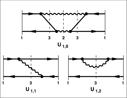
Figure 1: The three graphs of the effective interaction in the $q\bar{q}$-space. The lower two graphs correspond to the chain $U=VG_{3}V$, the upper corresponds to $U_{a}=VG_{3}VG_{2}VG_{3}V$. Propagator boxes are represented by vertical dashed lines, with the subscript ‘$n$’ referring to the sector numbers.

The method of iterated resolvents was applied in [26] to the paradigmatic case of a $4\times 4$-matrix, including explicit numerical examples. Applying the method to the block matrix structure of QCD, as displayed in Table 1, is particularly easy and transparent. By definition, the last sector contains only the diagonal kinetic energy, thus $H_{13}=T_{13}$. Its resolvent is calculated trivially. Then $H_{12}$ can be constructed unambiguously, followed by $H_{11}$, and so on, until one arrives at sector 1. Grouping them in a different order, one finds for the sectors with one $q\bar{q}$-pair:

$$H_{q\bar{q}}=\qquad H_{1} = T_{1}+\phantom{[}VG_{3}V+VG_{3}VG_{2}VG_{3}V\phantom{]}\ ,$$ (18)

$$H_{q\bar{q}\,g}=\qquad H_{3} = T_{3}+\phantom{[}VG_{6}V+VG_{6}VG_{5}VG_{6}V\phantom{]}+VG_{4}V\ ,$$ (19)

$$H_{q\bar{q}\,gg}=\qquad H_{6} = T_{6}+\phantom{[}VG_{10}V+VG_{10}VG_{9}VG_{10}V\phantom{]}+VG_{7}V\ ,$$ (20)

$$H_{q\bar{q}\,ggg}=\qquad H_{10} = T_{10}+\left[VG_{15}V+VG_{15}VG_{14}VG_{15}V\right]+VG_{11}V\ .$$ (21)

The quark-gluon content of the respective sectors is added here for an easier identification. The square bracket in the last expression indicates how the effective interaction looks for a higher $K$; for $K=4$ the content of the square bracket has to be set to zero. Correspondingly, one obtains for the sectors with two $q\bar{q}$-pairs:

$$H_{q\bar{q}q\bar{q}}=\qquad H_{4} = T_{4}+\phantom{[}VG_{7}V+VG_{7}VG_{6}VG_{7}V\phantom{]}\ ,$$ (22)

$$H_{q\bar{q}q\bar{q}\,g}=\qquad H_{7} = T_{7}+\phantom{[}VG_{11}V+VG_{11}VG_{10}VG_{11}V\phantom{]}+VG_{8}V\ ,$$ (23)

$$H_{q\bar{q}q\bar{q}\,gg}=\qquad H_{11} = T_{11}+\left[VG_{16}V+VG_{16}VG_{15}VG_{16}V\right]+VG_{12}V\ ,$$ (24)

and for those with with three $q\bar{q}$-pairs

$$H_{q\bar{q}q\bar{q}q\bar{q}}=\qquad H_{8} = T_{8}+VG_{12}V+\phantom{[}VG_{12}VG_{11}VG_{12}V\phantom{]}\ ,$$ (25)

$$H_{q\bar{q}q\bar{q}q\bar{q}\,g}=\qquad H_{12} = T_{12}+\left[VG_{17}V+VG_{17}VG_{16}VG_{12}V\right]+VG_{13}V\ .$$ (26)

In either case, their structure is different from the one in the pure glue sectors which is

$$H_{gg}=\qquad H_{2} = T_{2}+VG_{3}V+\phantom{[}VG_{5}V\phantom{]}\ ,$$ (27)

$$H_{gg\,g}=\qquad H_{5} = T_{5}+VG_{6}V+\phantom{[}VG_{9}V\phantom{]}\ ,$$ (28)

$$H_{gg\,gg}=\qquad H_{9} = T_{9}+VG_{10}V+\left[VG_{14}V\right]\ .$$ (29)

Having arrived at this point, one can restore first the limit $K\longrightarrow\infty$, simply by suppressing the square brackets in the above relations. Second, the instantaneous interaction $W$ omitted thus far can be restored ex post. Due to the peculiar structure of the gauge theory Hamiltonian displayed in Table 1, the vertex interaction appears only in even pairs, typically in the combination $VGV$. It is plausible that by simply substituting $VGV\rightarrow W+VGV$ restores the full Hamiltonian $H=T+V+W$, as was checked explicitly in [26].

The full effective Hamiltonian $H_{\rm eff}=H_{q\bar{q}}$ is given by Eq.(18) and displayed diagrammatically in Fig. 1. What does it mean physically? The first term is the kinetic energy ($T_{1}$) in the $q\bar{q}$-space. In the second term ($VG_{3}V$), the vertex interaction $V$ creates a gluon and scatters the system from the $q\bar{q}$- into the $q\bar{q}\,g$-space. As indicated in Fig. 1 by the vertical line with the subscript ‘3’, the three particles propagate there in ‘3’-space under impact of the full interaction before the gluon is absorbed. The gluon can be absorbed either by the antiquark or by the quark, represented by the two respective graphs $U_{1,1}$ and $U_{1,2}$ in the figure. The third term ($VG_{3}VG_{2}VG_{3}V$), finally, in Eq.(18) describes the virtual annihilation of the $q\bar{q}$-pair into two gluons, and is represented by the graph $U_{1,0}$ in Fig. 1. It generates an interaction between different quark flavors. As a net result the interaction scatters a quark with helicity $\lambda_{q}$ and four-momentum $p=(xP^{+},x\vec{P}_{\!\perp}+\vec{k}_{\!\perp},p^{-})$ into a state with $\lambda_{q}^{\prime}$ and four-momentum ${p^{\prime}}=(x^{\prime}P^{+},x^{\prime}\vec{P}_{\!\perp}+\vec{k}_{\!\perp}^{\prime},{p^{\prime}}^{-})$, and correspondingly the antiquark.

In the continuum limit, the resolvents are replaced by propagators and the eigenvalue problem $H_{\rm eff}|\psi\rangle=M^{2}|\psi\rangle$ becomes again an integral equation but one with a more transparent structure:

$$M_{b}^{2}\langle x,\vec{k}_{\!\perp};\lambda_{q},\lambda_{\bar{q}}|\psi_{b}\rangle=\left[{\overline{m}^{2}_{q}+\vec{k}_{\!\perp}^{2}\over x}+{\overline{m}^{2}_{\bar{q}}+\vec{k}_{\!\perp}^{2}\over 1-x}\right]\langle x,\vec{k}_{\!\perp};\lambda_{q},\lambda_{\bar{q}}|\psi_{b}\rangle$$

$$+\sum_{\lambda_{q}^{\prime},\lambda_{\bar{q}}^{\prime}}\!\int_{D}\!dx^{\prime}d^{2}\vec{k}_{\!\perp}^{\prime}\,\langle x,\vec{k}_{\!\perp};\lambda_{q},\lambda_{\bar{q}}|U+U_{a}|x^{\prime},\vec{k}_{\!\perp}^{\prime};\lambda_{q}^{\prime},\lambda_{\bar{q}}^{\prime}\rangle\,\langle x^{\prime},\vec{k}_{\!\perp}^{\prime};\lambda_{q}^{\prime},\lambda_{\bar{q}}^{\prime}|\psi_{b}\rangle \ .$$ (30)

The effective quark mass $\overline{m}$ includes the impact of diagram $U_{1,2}$. The domain $D$ restricts integration in line with regularization (see below). The effective interaction $U$ includes all fine and hyperfine interactions. The flavor-changing annihilation interaction $U_{a}=U_{1,0}$ is probably of less importance in a first assault and will be disregarded in the sequel. The eigenvalues refer to the invariant mass $M_{b}$ of a physical state and the corresponding wavefunction $\langle x,\vec{k}_{\!\perp};\lambda_{q},\lambda_{\bar{q}}|\psi_{b}\rangle$ gives the probability amplitudes for finding in that state a flavored quark with momentum fraction $x$, intrinsic transverse momentum $\vec{k}_{\!\perp}$ and helicity $\lambda_{q}$. Both are boost-invariant quantities. Color plays a subordinate role because the Fock states can be made color-neutral.

The eigenfunctions $\psi_{b}$ represent the normalized projections of the full eigenfunction $|\Psi\rangle$ onto the Fock states $|q;\bar{q}\rangle=b^{\dagger}_{q}d^{\dagger}_{\bar{q}}|vac\rangle$. Their knowledge is sufficient to retrieve all desired Fock-space components of the total wavefunction $|\Psi\rangle$. Let us work that out explicitly by asking for the probability amplitude to find a $|gg\rangle$- or a $|q\bar{q}\,g\rangle$-state in an eigenstate $|\Psi\rangle$ of the full Hamiltonian. The key is the upwards recursion relation Eq.(16). Obviously, one can express the higher Fock-space components $\langle n|\Psi\rangle$ as functionals of $\psi_{q\bar{q}}$ by a finite series of quadratures, i.e. of matrix multiplications or of momentum-space integrations. One needs not solve another eigenvalue problem. The first two equations of the recursive set in Eq.(16) are

$$\langle 2|\Psi\rangle = G_{2}\langle 2|H_{2}|1\rangle\langle 1|\Psi\rangle\,,$$ (31)

$${\rm and}\quad\langle 3|\Psi\rangle = G_{3}\langle 3|H_{3}|1\rangle\langle 1|\Psi\rangle+G_{3}\langle 3|H_{3}|2\rangle\langle 2|\Psi\rangle\,.$$ (32)

The sector Hamiltonians $H_{n}$ have to be substituted from Eqs.(19) and (27). In taking block matrix elements of them, the formal expressions are simplified considerably since many of the Hamiltonian blocks in Table 1 are zero. One thus gets simply $\langle 2|H_{2}|1\rangle=\langle 2|VG_{3}V|1\rangle$ and therefore $\langle 2|\Psi\rangle=G_{2}VG_{3}V\langle 1|\Psi\rangle$. Substituting this into Eq.(31) gives $\langle 3|\Psi\rangle=G_{3}V\langle 1|\Psi\rangle+G_{3}VG_{2}VG_{3}V\langle 1|\Psi\rangle$. These findings can be summarized more readable as

$$|\psi_{gg}\rangle = G_{gg}VG_{q\bar{q}\,g}V\>|\psi_{q\bar{q}}\rangle,$$ (33)

$${\rm and}\qquad|\psi_{q\bar{q}\,g}\rangle = G_{q\bar{q}\,g}V\>|\psi_{q\bar{q}}\rangle+G_{q\bar{q}\,g}VG_{gg}VG_{q\bar{q}\,g}V\>|\psi_{q\bar{q}}\rangle\ .$$ (34)

Correspondingly, one can write down the higher Fock-space wavefunctions as functionals of only $|\psi_{q\bar{q}}\rangle$. Of course, one has to readjust the overall normalization of the wavefunction, and this depends on how many Fock spaces one decides to include. Finally, it should be emphasized again that the finite number of terms contrasts strongly to the infinite number of terms in perturbative series, because the iterated resolvents re-sum the series to all orders in closed form. The above results are all exact.

Aiming for the higher Fock space amplitudes is not an esoteric problem. One needs them for calculating the structure functions, for example. They are the probability amplitudes for finding in a hadron a quark with longitudinal momentum fraction $x$, irrespective of its transverse momentum, and to get them, one must sum over all Fock-space amplitudes $f(x)=\sum_{n}\langle\overline{\Psi}_{n}|b^{\dagger}(x)b(x)|\Psi_{n}\rangle$, see for example [12].

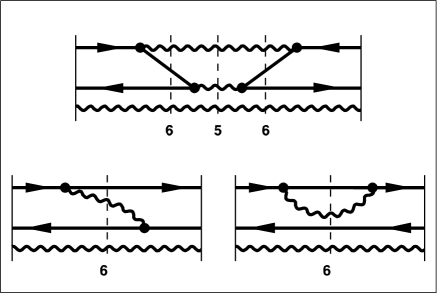
Figure 2: The three graphs of the spectator interaction in the $q\bar{q}\,g$-space. Note the role of the gluon as a spectator.

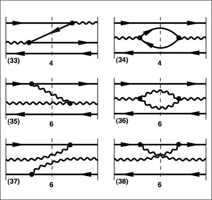
Figure 3: Some six graphs of the participant interaction in the $q\bar{q}\,g$-space.

Let us discuss in some greater detail the structure of the sector Hamiltonians, particularly the effective interaction in the ${q\bar{q}\,g}$-space as given by Eq.(19). The corresponding graphs are displayed diagrammatically in Figs. 3 and 3. Those in Fig. 3 differ from those in Fig. 1 only by an additional gluon. The gluon does not change quantum numbers under impact of the interaction and acts like a spectator. Therefore, the graphs in Fig. 3 will be referred to as the ‘spectator interaction’ $\overline{U}_{3}$. In the graphs of Fig. 3, the gluons are scattered by the interaction, and correspondingly these graphs will be referred to as the ‘participant interaction’ $\widetilde{U}_{3}$. The analogous separation into spectators and participants can be made in all quark-pair-glue sector Hamiltonians:

$$H_{n}=T_{n}+\overline{U}_{n}+\widetilde{U}_{n}\ ,\quad{\rm for}\quad n=3,6,10,15,\dots\ .$$ (35)

The Hamiltonian is additive in spectators and participants. The spectator interaction $\overline{U}_{n}$ therefore can be associated with its own resolvent $\overline{G}_{n}$,

$$\overline{G}_{n}={1\over\omega-T_{n}-\overline{U}_{n}}\,,\qquad\biggl{(}{\rm while\ }G_{n}\equiv{1\over\omega-H_{n}}={1\over\omega-T_{n}-\overline{U}_{n}-\widetilde{U}_{n}}\ \biggr{)}\,,$$ (36)

with an exact relation to the full resolvents $G_{n}$, i.e. $G_{n}=\overline{G}_{n}+\overline{G}_{n}\,\widetilde{U}_{n}\,G_{n}$. Equivalently, one can write it as an infinite series $G_{n}=\overline{G}_{n}+\overline{G}_{n}\widetilde{U}_{n}\,\overline{G}_{n}+\overline{G}_{n}\widetilde{U}_{n}\,\overline{G}_{n}\widetilde{U}_{n}\,\overline{G}_{n}+\dots$, as usual. The difference to the usual perturbative series in Sec. 2 is, that there the ‘unperturbed propagator’ $G_{0}(\omega)$ refers to the system without interactions while here the ‘unperturbed propagators’ $\overline{G}_{n}$ contain the interaction in the well defined form of $\overline{U}_{n}$. One therefore deals here with a ‘perturbation theory in medium’. Note that the present series implies also different physics: The system is not scattered into other sectors but stays in sector $n$. This is reflected in the operator identity, which is obtained straightforwardly from Eqs.(35) and (36):

$$(1-\widetilde{U}_{n}\overline{G}_{n})(\omega-\overline{H}_{n})=\left(1-\widetilde{U}_{n}{1\over\omega-\overline{H}_{n}}\right)(\omega-\overline{H}_{n})=\omega-H_{n}\ .$$ (37)

Taking the inverse gives $G_{n}=\overline{G}_{n}R_{n}^{2}$, thus

$$R_{n}^{2}={1\over 1-\overline{G}_{n}\widetilde{U}_{n}}\ .$$ (38)

Since $R_{n}$ and $\overline{G}_{n}$ commute, one ends up with $G_{n}=R_{n}\,\overline{G}_{n}\,R_{n}$. In all of the above effective interactions the square matrices $R_{n}$ are sandwiched between a quark-pair-glue resolvent $\overline{G}$ and the vertex $V$,

$$V\,G_{n}\,V=V\,R_{n}\,\overline{G}_{n}\,R_{n}\,V=\overline{V}\,\overline{G}_{n}\,\overline{V}\,,$$ (39)

with $\overline{V}=R_{n}V$ being an effective vertex. The index $n$ needs not to be carried on. One can thus rewrite systematically Eqs.(18)-(21). Working backwards yields

$$\overline{H}_{6} = T_{6}+\overline{V}\,\overline{G}_{10}\overline{V}+\overline{V}\,\overline{G}_{10}\overline{V}G_{9}\overline{V}\,\overline{G}_{10}\overline{V}\ ,$$ (40)

$$\overline{H}_{3} = T_{3}+\overline{V}\,\overline{G}_{6}\overline{V}+\overline{V}\,\overline{G}_{6}\overline{V}G_{5}\overline{V}\,\overline{G}_{6}\overline{V}\ ,$$ (41)

$$H_{1}=\overline{H}_{1} = T_{1}+\overline{V}\,\overline{G}_{3}\overline{V}+\overline{V}\,\overline{G}_{3}\overline{V}G_{2}\overline{V}\,\overline{G}_{3}\overline{V}\ .$$ (42)

Instead of being similar, the quark-pair-glue sector Hamiltonians $\overline{H}_{n}=T_{n}+\overline{U}_{n}$ are now all identical. Note that, in the strict sense, they are equal only in the continuum limit. For any finite $K$, there is a last sector which is creating edge effects. The resolvents $G_{2}$, $G_{5}$ and $G_{9}$ carry no bar. In the pure glue sectors, the distinction between participants and spectators makes no sense.

4 Analysis of propagators and vertex functions

Thus far the approach is formally exact. In the sequel, this rigor is given up in favor of transparency. For calculating the effective interaction $U$ one needs the resolvents $\overline{G}_{3}$. For calculating $\overline{G}_{3}$, one needs $\overline{G}_{4}$ and $\overline{G}_{6}$, and so one. Does this ever come to an end? A careful analysis shows that there is a simple relation between them since all $\overline{H}_{n}(\omega)$ are all bona fide Hamiltonians. Suppose we have solved the eigenvalue problem in the $q\bar{q}$-space,

$$\sum_{q^{\prime},\bar{q}^{\prime}}\langle q;\bar{q}|H_{q\bar{q}}(\omega)|q^{\prime};\bar{q}^{\prime}\rangle\,\langle q^{\prime};\bar{q}^{\prime}|\psi_{b}(\omega)\rangle=M_{b}^{2}(\omega)\langle q;\bar{q}|\psi_{b}(\omega)\rangle\,.$$ (43)

The eigenvalues are enumerated by $b=1,2,\dots\infty$. The eigenfunctions $\langle q;\bar{q}|\psi_{b}(\omega)\rangle$ are a complete set. Despite working in the continuum limit, we continue to use summation symbols for the sake of a more compact notation. Suppose further that an $\omega$ was found which has the same value as the lowest eigenvalue $M^{2}=M^{2}_{1}$. The substitution $\omega=M^{2}$ will hence forward be done without explicitly mentioning. Next, ask for the eigenvalues and eigenfunctions in the $q\bar{q}\,g$-space:

$$\sum_{q^{\prime},\bar{q}^{\prime},g^{\prime}}\langle q;\bar{q};g|\overline{H}_{3}|q^{\prime};\bar{q}^{\prime};g^{\prime}\rangle\langle q^{\prime};\bar{q}^{\prime};g^{\prime}|\psi_{b,s}\rangle=M_{b,s}^{2}\langle q;\bar{q};g|\psi_{b,s}\rangle\,.$$ (44)

It is important to note that one needs not to perform another calculation, becuase the result is already known. By construction, the gluon is a free particle which moves relative to the meson subject to momentum conservation. The eigenfunction is a product state $|\psi_{b,s}\rangle=|\psi_{b}\rangle\otimes|\varphi_{s}\rangle$. Parameterizing the gluon’s four-momentum as

$$q_{g}^{\mu}=(yP^{+},y\vec{P}_{\!\perp}+\vec{q}_{\!\perp},p_{g}^{-})$$ (45)

implies that the gluon moves with momentum fraction $y$ and transverse momentum $\vec{q}_{\!\perp}$. It also implies that the meson moves with momentum fraction $1-y$ and transverse momentum $-\vec{q}_{\!\perp}$. Since the gluons are massless, the eigenvalues are therefore

$$M_{b,s}^{2}={M_{b}^{2}+\vec{q}_{\!\perp}^{\,2}\over(1-y)}+{\vec{q}_{\!\perp}^{\,2}\over y}\,.$$ (46)

Knowing the eigenvalues and eigenfunctions, one can calculate the exact resolvent. A few identical rewritings give

$$\langle q;\bar{q};g|\overline{G}_{3}|q^{\prime};\bar{q}^{\prime};g^{\prime}\rangle = \overline{G}_{3}(q;\bar{q};g)\left[\langle q;\bar{q};g|q^{\prime};\bar{q}^{\prime};g^{\prime}\rangle-\langle q;\bar{q};g|A|q^{\prime};\bar{q}^{\prime};g^{\prime}\rangle\right]\,,\qquad{\rm with}$$ (47)

$$A = \sum_{b,s}|\psi_{b,s}\rangle\,{y(M_{b}^{2}-M^{2})\over Q^{2}+y(M_{b}^{2}-M^{2})}\,\langle\psi_{b,s}|\,,$$ (48)

$$\overline{G}_{3}(q;\bar{q};g) = -{y\over Q^{2}}\ ,\quad{\rm and}\quad Q^{2}=(y^{2}M^{2}+\vec{q}_{\!\perp}^{\,2}){1\over 1-y}\,.$$ (49)

Since the operator $A$ by definition cannot become a Dirac-$\delta$ function $\langle q;\bar{q};g|q^{\prime};\bar{q}^{\prime};g^{\prime}\rangle$, one can drop $A$, as an approximation. The same type of approximation parametrizes the two gluon propagator $\overline{G}_{2}(g_{1};g_{2})=(M^{2}-M^{2}_{gb})^{-1}$ in terms of the glue ball mass $M^{2}_{gb}$.

Let us digress for a short discussion. One should note first that the above approximation can be controlled e posteriori: Once the eigenfunctions in the $q\bar{q}$-sector are available numerically, one can check whether the exact definition of the resolvent Eq.(47) is peaked like a $\delta$-function, with a residue predicted by Eq.(49). Second, the above notation is suggestive for $Q^{2}$ being related to the single-particle four-momentum transfer along the quark line in graph $U_{1,1}$ in Figure 1. In fact one gets $(p-p^{\prime})^{2}=-[y^{2}(2m)^{2}+\vec{q}_{\!\perp}^{\,2}]$, for sufficiently small $y$. The momentum transfer is the same as in Eq.(49) if one replaces the ‘current mass’ $m$ by the ‘constituent mass’ $M/2$. Apart from that the exact resolvent agrees with the perturbative propagator: In the solution, the particles propagate like free particles. Third, and most importantly, instead of having resolvents of resolvents, the hierarchy of iterated resolvents is broken. Ex post, this justifies the ad-hoc procedures in the Tamm-Dancoff approach, both in the original work [23, 24] and in its light-cone adaption [22, 28]. Last but not least, one should emphasize that the complicated operator $A$ in Eq.(47) can perhaps be omitted when dealing with the low energy part of the spectrum. This becomes inadequate if not false at sufficiently high excitations, at sufficiently large $\omega$, where one might be in the region of ‘overlapping resonances’ [29]. This requires different techniques, possibly those based on random matrix models [30, 31]. It is here where the concept of a temperature will possibly make its way into the Hamiltonian bound-state problem.

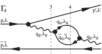
Figure 4: The $q\bar{q}$ vacuum polarization graph.

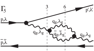
Figure 5: The $gg$ vacuum polarization graph.

Next, how can one approximate the vertex functions $R_{n}$? With Eq.(37) one has

$$R_{n}=1+{1\over 2}\overline{G}_{n}\widetilde{U}_{n}+{3\over 8}\overline{G}_{n}\widetilde{U}_{n}\,\overline{G}_{n}\widetilde{U}_{n}+\dots\,.$$ (50)

For $n=3$, this reads $R_{3}=(1-\overline{G}_{3}[VR_{6}\overline{G}_{6}R_{6}V+VR_{4}\overline{G}_{4}R_{4}V])^{-{1\over 2}}$. Expanding up to the first non-trivial term in the expansion gives

$$R_{3}\simeq 1+{1\over 2}\left(\overline{G}_{3}V\overline{G}_{4}V+\overline{G}_{3}V\overline{G}_{6}V\right)=1+{1\over 2}\left(\Gamma_{1}+\Gamma_{2}+\Gamma_{3}+\Gamma_{4}+\Gamma_{5}\right)\ .$$ (51)

For being consistent one must set $R_{4}=R_{6}=1$. Unfortunately, this was not realized in the previous work [26]. The vertex function $R_{3}$ identifies itself as the conventional vertex function. The altogether 5 diagrams of light-cone QCD had been calculated before by Thorn [32] and by Perry [33]. Because they are not available in the form we need them in the sequel, we have recalculated them and present them elsewhere [34]. In the nomenclature of [33], the mass term $\Gamma_{1}$ cancels almost completely with the two vertex corrections $\Gamma_{2}$ and $\Gamma_{3}$. In the sequel we consider explicitly only the two vacuum polarization diagrams $\Gamma_{4}$ and $\Gamma_{5}$, as given in Figs. 5 and 5. Parameterizing the particle momenta as

$$q_{q}^{\mu} = \left(yzP^{+},\ yz\vec{P}_{\!\perp}+z\vec{q}_{\!\perp}+\vec{l}_{\!\perp},\ p_{g_{1}}^{-}\right)\ ,$$

$$\bar{q}_{\bar{q}}^{\mu} = \left(y(1-z)P^{+},\ y(1-z)\vec{P}_{\!\perp}+(1-z)\vec{q}_{\!\perp}-\vec{l}_{\!\perp},\ p_{g_{2}}^{-}\right)\,,$$ (52)

we calculate first the propagators in the $q\bar{q}\,q\bar{q}$ and $q\bar{q}\,gg$ sectors,

$$\overline{G}_{q\bar{q}\,q\bar{q}}=\overline{G}_{4} = -{q_{g}^{+}\over P^{+}}{z(1-z)\over z(1-z)Q^{2}+\vec{l}_{\!\perp}^{\,2}+m^{2}_{f}}\,,\quad{\rm and}$$ (53)

$$\overline{G}_{q\bar{q}\,gg}=\overline{G}_{6} = -{q_{g}^{+}\over P^{+}}{z(1-z)\over z(1-z)Q^{2}+\vec{l}_{\!\perp}^{\,2}}\ .$$ (54)

They depend on $Q^{2}$, the momentum transfer along the quark line. The vacuum polarization diagrams are then calculable according to the rules of light-cone perturbation theory [12] and yield

$$\Gamma_{4} = -\sum_{f}{\alpha\over 4\pi}\int\!dz\,dl_{\perp}^{2}\ \Theta_{s}\ {1-2z(1-z)-{2m_{f}^{2}\over Q^{2}}\over l_{\perp}^{2}+m_{f}^{2}+z(1-z)Q^{2}}\,,$$ (55)

$$\Gamma_{5} = \phantom{-\sum_{f}}{\alpha n_{c}\over 2\pi}\int\!dz\,dl_{\perp}^{2}\ \Theta_{g}\ {2-z(1-z)-{1\over z(1-z)}\over l_{\perp}^{2}+z(1-z)Q^{2}}\,.$$ (56)

The dependence on $Q^{2}$ is caused by the propagators. The term with $1/z(1-z)$ in $\Gamma_{5}$ cancels with $\Gamma_{1}+\Gamma_{2}+\Gamma_{3}$, like in the previous work [32, 33]. These authors have however not kept track of the $Q^{2}$-dependence. Dropping this term replaces $\Gamma_{5}$ with $\overline{\Gamma}_{5}$. The cut-off functions $\Theta$ are defined by vertex regularization in Eq.(4) and (5)

$$\Theta(z,l_{\!\perp}^{2})=\cases{1,&for $\ 0\leq l_{\!\perp}^{2}\leq l^{2}_{\Lambda}(z)$ and $\ \epsilon_{l}\leq z\leq 1-\epsilon_{u}\ $ ,\cr 0,&otherwise.\cr}$$ (57)

The limiting transverse momentum $l_{\Lambda}^{2}(z)$ describes a semi-circle in the appropriate units,

$$l_{\Lambda}^{2}(z) = \big{(}\Lambda^{2}+(m_{1}+m_{2})^{2}\big{)}\bigg{[}\bigg{(}{c\over 2}\bigg{)}^{2}-\bigg{(}z-{b\over 2}\bigg{)}^{2}\bigg{]}$$

$$\quad{\rm with}\quad b = {\Lambda^{2}+2m_{1}(m_{1}+m_{2})\over\Lambda^{2}+(m_{1}+m_{2})^{2}}\quad{\rm and}\quad c^{2}={\Lambda^{2}\over\Lambda^{2}+(m_{1}+m_{2})^{2}}{\Lambda^{2}+4m_{1}m_{2}\over\Lambda^{2}+(m_{1}+m_{2})^{2}}\,.$$ (58)

The semi-circle is limited by its intersections at $z_{1}=\epsilon_{l}$ and $z_{2}=1-\epsilon_{u}$, with

$$\epsilon_{l}={b-c\over 2}\quad{\rm and}\quad\epsilon_{u}=1-{b+c\over 2}\,.$$ (59)

For sufficiently large $\Lambda$ and equal masses $m_{1}=m_{2}=m$, the limits become $\epsilon_{l}=\epsilon_{u}=(m/\Lambda)^{2}$. For the purpose of regularization, the gluons are endorsed with a small mass $m_{g}$, and thus vertex regularization regulates all divergences on the light cone. One gets straightforwardly

$$\Gamma_{4}=-\sum_{f}{\alpha\over 4\pi}\int\limits_{\epsilon_{f}}^{1-\epsilon_{f}}\!\!\!dz\,\bigg{(}1-2z(1-z)-{2m_{f}^{2}\over Q^{2}}\bigg{)}\ \ln{{\Lambda^{2}+4m_{f}^{2}+Q^{2}\over Q^{2}+{m_{f}^{2}\over z(1-z)}}}\,.$$ (60)

This is approximated by replacing the term $m_{f}^{2}/z(1-z)$ by its maximum at $z={1\over 2}$, that is by $4m_{f}^{2}$. The same type of approximation is done for $\Gamma_{5}$, yielding finally

$$\Gamma_{4}=\sum_{f}{\alpha\over 6\pi}\bigg{(}{3m_{f}^{2}\over Q^{2}}-1\bigg{)}\ln{\bigg{(}1+{\Lambda^{2}\over 4m_{f}^{2}+Q^{2}}\bigg{)}}\,,\quad{\rm and}\quad\overline{\Gamma}_{5}={11\alpha n_{c}\over 12\pi}\ln{\bigg{(}1+{\Lambda^{2}\over 4m_{g}^{2}+Q^{2}}\bigg{)}}\,.$$ (61)

In either case, the terms depending on $\epsilon_{f}=(m_{f}/\Lambda)^{2}$ or $\epsilon_{g}=(m_{g}/\Lambda)^{2}$ have been dropped since they are small. The effective coupling constant $\overline{\alpha}_{s}\equiv\alpha R^{2}_{3}=\alpha(1+\Gamma_{4}+\overline{\Gamma}_{5})$,

$$\overline{\alpha}_{s}(Q^{2})=\alpha+{11\alpha^{2}n_{c}\over 12\pi}\ln{\bigg{(}1+{\Lambda^{2}\over 4m_{g}^{2}+Q^{2}}\bigg{)}}+{\alpha^{2}\over 6\pi}\sum_{f}\bigg{(}{3m_{f}^{2}\over Q^{2}}-1\bigg{)}\ln{\bigg{(}1+{\Lambda^{2}\over 4m_{f}^{2}+Q^{2}}\bigg{)}}\,,$$ (62)

depends therefore on the momentum transfer. Finally, the effective quark and gluon masses become

$$\overline{m}_{f}^{2}=m_{f}^{2}+m_{f}^{2}{\alpha\over\pi}{n_{c}^{2}-1\over 2n_{c}}\ln{{\Lambda^{2}\over m_{g}^{2}}}\,,\quad{\rm and}\quad\overline{m}_{g}^{2}=m_{g}^{2}-{\alpha\over 4\pi}\sum_{f}m_{f}^{2}\ \ln{\bigg{(}1+{\Lambda^{2}\over 4m_{f}^{2}}\bigg{)}}\,.$$ (63)

They are obtained straightforwardly by light-cone perturbation theory [12] combined with vertex regularization. The diagram for the effective quark mass $\overline{m}_{f}^{2}=m_{f}^{2}(1+\Gamma_{6})$ is given in Fig. 7. There is a corresponding diagram for the effective gluon mass $\overline{m}_{g}^{2}$.

5 Renormalization group analysis and confinement

Collecting terms and restricting to $n_{c}=3$ colors, the effective interaction as defined in Eq.(30) becomes without the flavor changing interaction $U_{a}$

$$E\ \langle x,\vec{k}_{\!\perp};\lambda_{q},\lambda_{\bar{q}}|\psi\rangle=\left[{\overline{m}^{\,2}_{q}+\vec{k}_{\!\perp}^{\,2}\over x}+{\overline{m}^{\,2}_{\bar{q}}+\vec{k}_{\!\perp}^{\,2}\over 1-x}\right]\langle x,\vec{k}_{\!\perp};\lambda_{q},\lambda_{\bar{q}}|\psi\rangle$$

$$-{1\over 3\pi^{2}}\sum_{\lambda_{q}^{\prime},\lambda_{\bar{q}}^{\prime}}\!\int_{D}\!dx^{\prime}d^{2}\vec{k}_{\!\perp}^{\prime}\,\,{\overline{\alpha}_{s}(Q)\over Q^{2}}\,\langle\lambda_{q},\lambda_{\bar{q}}|S(Q)|\lambda_{q}^{\prime},\lambda_{\bar{q}}^{\prime}\rangle\ \langle x^{\prime},\vec{k}_{\!\perp}^{\prime};\lambda_{q}^{\prime},\lambda_{\bar{q}}^{\prime}|\psi\rangle \,.$$ (64)

One recalls that the four-momentum transfer along the quark (or anti-quark) line is $Q^{2}=-(k_{q}-k_{q}^{\prime})^{2}=-(k_{\bar{q}}-k_{\bar{q}}^{\prime})^{2}\simeq(m_{q}+m_{\bar{q}})^{2}(x-x^{\prime})^{2}+(\vec{k}_{\!\perp}-\vec{k}_{\!\perp}^{\prime})^{2}$. As we are supposed to do, we restore the instantaneous interaction $W$ in the $q\bar{q}$-space when deriving the above result, thus $\overline{U}_{q\bar{q}}=W_{q\bar{q}}+\overline{V}\,\overline{G}_{q\bar{q}\,g}\overline{V}$. Both the instantaneous interaction $W$ and the vertex interaction $\overline{V}\,\overline{G}_{q\bar{q}\,g}\overline{V}$ have a non-integrable singularity, cf [12], which cancels each other such that only the integrable Coulomb singularity remains. The latter manifests itself in Eq.(64) in the “Coulomb denominator” $Q^{-2}$. The spinor factor $S(Q)$ represents the familiar current-current coupling which describes all fine and hyperfine interactions

$$\,\langle\lambda_{q},\lambda_{\bar{q}}|S(Q)|\lambda_{q}^{\prime},\lambda_{\bar{q}}^{\prime}\rangle\,={\left[\overline{u}(k_{q},\lambda_{q})\,\gamma^{\mu}\,u(k_{q}^{\prime},\lambda_{q}^{\prime})\right]\over\sqrt{xx^{\prime}}}\,{\left[\overline{u}(k_{\bar{q}},\lambda_{\bar{q}})\,\gamma_{\mu}\,u(k_{\bar{q}}^{\prime},\lambda_{\bar{q}}^{\prime})\right]\over\sqrt{(1-x)(1-x^{\prime})}}\,.$$ (65)

One can simplify the expression technically by suppressing in the latter all momentum dependence. Evaluating the spinors at equilibrium, i.e. at vanishing transverse momenta and at momentum fractions $\bar{x}_{q}=m_{q}/(m_{q}+m_{\bar{q}})$ and $\bar{x}_{\bar{q}}=m_{\bar{q}}/(m_{q}+m_{\bar{q}})$, gives [12]

$${\left[\overline{u}(k_{q},\lambda_{q})\,\gamma^{\mu}\,u(k_{q}^{\prime},\lambda_{q}^{\prime})\right]\over\sqrt{x_{q}x_{q}^{\prime}}}{\left[\overline{u}(k_{\bar{q}},\lambda_{\bar{q}})\,\gamma_{\mu}\,u(k_{\bar{q}}^{\prime},\lambda_{\bar{q}}^{\prime})\right]\over\sqrt{x_{\bar{q}}x_{\bar{q}}^{\prime}}}\bigg{|}_{\rm equilibrium}=4(m_{q}+m_{\bar{q}})^{2}\,\delta_{\lambda_{q},\lambda_{q}^{\prime}}\delta_{\lambda_{\bar{q}},\lambda_{\bar{q}}^{\prime}}\,.$$ (66)

Omitting the spin-dependence of the interaction implies to restrict oneselve to the central part of the interaction. In this approximation Eq.(64) becomes

$$E\ \langle x,\vec{k}_{\!\perp}|\psi\rangle=\left[{\overline{m}^{\,2}_{q}+\vec{k}_{\!\perp}^{\,2}\over x}+{\overline{m}^{\,2}_{\bar{q}}+\vec{k}_{\!\perp}^{\,2}\over 1-x}\right]\langle x,\vec{k}_{\!\perp}|\psi\rangle-{4(m_{q}+m_{\bar{q}})^{2}\over 3\pi^{2}}\int_{D}\!\!\!dx^{\prime}d^{2}\vec{k}_{\!\perp}^{\prime}\,{\overline{\alpha}_{s}(Q)\over Q^{2}}\ \langle x^{\prime},\vec{k}_{\!\perp}^{\prime}|\psi\rangle\,.$$ (67)

It is this equation, finally, which we are going to analyze by the renormalization group.

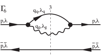
Figure 6: The quark mass diagram.

$m_{u}=$	6 MeV
$m_{d}=$	10 MeV
$m_{s}=$	200 MeV
$m_{c}=$	1.40 GeV
$m_{b}=$	4.70 GeV
$m_{t}=$	180 GeV
$\alpha=$	0.2
$\Lambda=$	100 MeV
$m_{g}=$	13 MeV

Figure 7: Fixing the bare quantities.

In order to do calculations, one has to specify 10 “input parameters”. As specified in Fig. 7, these are the six flavor masses $m_{f}$ [35], the coupling constant $\alpha=g^{2}/4\pi$, and the two regularization parameters $\Lambda$ and $m_{g}$. To be concrete, these parameters are specified in Fig. 7, and subject to future change. The eigenvalues of the effective equation (67) depend on all of them, i.e. $E_{i}(m_{f},\alpha;\Lambda,m_{g})$. While their dependence on the masses and coupling constant is not unexpected, they should not depend on $\Lambda$, since that is an arbitrary and unphysical parameter. One therefore must require that the eigenvalues satisfy the renormalization group equations

$${d\over d\Lambda}\,E_{i}(m_{f},\alpha;\Lambda,m_{g})=0\,.$$ (68)

Since the Lagrangian ‘bare’ parameters themselves are arbitrary, one can try to let them be functions of $\Lambda$ in order to satisfy Eq.(68): $m_{f}=m_{f}(\Lambda)$, $\alpha=\alpha(\Lambda)$, and $m_{g}=m_{g}(\Lambda)$. The numbers in Fig. 7 can be viewed as such functions at the particular value $\Lambda=100$ MeV. If one finds one single set of functions which makes all eigenvalues $E_{i}$ independent of $\Lambda$, one has solved the problem. It is not really necessary that $\Lambda\rightarrow\infty$.

In the present work, the eigenvalues of the full light-cone Hamiltonian $H_{LC}$ in Eq.(3) are conceptually identical with the eigenvalues of the effective Hamiltonian, Eq.(67). One must therefore analyze the latter. The dependence on the cut-off resides in three well separated locations: (1) in the domain of integration $D$, (2) in the effective coupling constant $\overline{\alpha}_{s}(Q,\Lambda)$, and (3) in the effective mass parameters $\overline{m}_{q}(\Lambda)$ and $\overline{m}_{\bar{q}}(\Lambda)$. As an advantage of vertex regularization, one can decouple the scales in $D$ and in the functions $\overline{\alpha}_{s}$ and $\overline{m}_{q}$. In the sequel we disregard the dependence on $D$.

If $\overline{\alpha}_{s}$ and $\overline{m}_{q}$ do not dependent on $\Lambda$, the eigenvalues cannot depend on $\Lambda$, either. It therefore suffices to require

$$\delta\overline{\alpha}_{s} = {\partial\overline{\alpha}_{s}\over\partial\alpha}\,\delta\alpha+{\partial\overline{\alpha}_{s}\over\partial\Lambda^{2}}\,\delta\Lambda^{2}+\sum_{f}{\partial\overline{\alpha}_{s}\over\partial m_{f}^{2}}\,\delta m_{f}^{2}\equiv 0\,,\quad{\rm and}$$ (69)

$$\delta\overline{m}_{f^{\prime}}^{2} = {\partial\overline{m}_{f^{\prime}}^{2}\over\partial\alpha}\,\delta\alpha+{\partial\overline{m}_{f^{\prime}}^{2}\over\partial\Lambda^{2}}\,\delta\Lambda^{2}+\sum_{f}{\partial\overline{m}_{f^{\prime}}^{2}\over\partial m_{f}^{2}}\,\delta m_{f}^{2}\equiv 0\,.$$ (70)

The variations of $\overline{\alpha}_{s}$ have to be performed of course at a fixed value of $Q^{2}$. Solving the corresponding differential equations for $\alpha(\Lambda)$ and $m_{f}^{2}(\Lambda)$ yields the required functions. There are two regimes which are particularly interesting. One is the asymptotic regime

$$m_{g}^{2},m_{f}^{2}\ll Q^{2}\ll\Lambda^{2}\,,$$ (71)

in which Eqs.(61) and (62) become

$$\overline{\alpha}_{s}=\alpha+\alpha^{2}a_{0}\ln{\Lambda^{2}\over Q^{2}}\,,\qquad{\rm with}\quad a_{0}={33-2n_{f}\over 12\pi}\,.$$ (72)

Solving Eq.(69) in this regime yields asymptotic freedom in the front form, as shown first by Thorn [32] and later by Perry et al. [33]. The asymptotic regime is particularly important for high energy scattering. But in a bound state calculation, the very large momentum transfers are less important than the very small ones, because of the Coulomb singularity $Q^{2}\sim 0$, see Eqs.(64) and (67). It provides the binding. In the sequel we therefore emphasize the bound state regime near $Q^{2}\sim 0$,

$$Q^{2}\ll m_{l}^{2}\ll\Lambda^{2}\ll m_{h}^{2}\,.$$ (73)

To our recollection, such a regime has not been analyzed by the renormalization group thus far. We shall differentiate between the two light quarks with mass $m_{l}$ (u,d) and the four heavy quarks with mass $m_{h}$ (s,c,b,t). For convenience we collect some mass parameters consistent with [35] in Fig. 7. In the present context, ‘light’ and ‘heavy’ is defined operationally by

$${m_{l}^{2}\over\Lambda^{2}}\ll 1\,,\quad{\rm and}\quad{m_{h}^{2}\over\Lambda^{2}}\gg 1\,.$$ (74)

Consider first the effective gluon mass. In a gauge theory the vector bosons should have zero mass $\overline{m}_{g}=0$. This in turn defines $m_{g}$

$$m_{g}^{2}={\alpha\over 4\pi}\sum_{h}m_{h}^{2}\ln{\bigg{(}1+{\Lambda^{2}\over 4m_{h}^{2}}\bigg{)}}+{\alpha\over 4\pi}\sum_{l}m_{l}^{2}\ \ln{\bigg{(}1+{\Lambda^{2}\over 4m_{l}^{2}}\bigg{)}}\,,$$ (75)

according to Eq.(63). Expanding the logarithm for the former gives

$$m_{g}^{2}={\alpha\over 4\pi}\Lambda^{2}\left(1+\sum_{l}{m_{l}^{2}\over\Lambda^{2}}\,\ln{\bigg{(}1+{\Lambda^{2}\over 4m_{l}^{2}}\bigg{)}}\right)\simeq{\alpha\over 4\pi}\Lambda^{2}\,.$$ (76)

With the parameter values of Fig. 7, the numbers in the parenthesis go like $(1+0.017)$. It is thus save to neglect the impact of the light quark masses. This yields $m_{g}\simeq 13$ MeV as quoted in the figure and removes the regulating gluon mass as a free parameter from the theory. In the vicinity of $Q^{2}\sim 0$, the effective coupling constant goes like

$$\overline{\alpha}_{s}={\alpha^{2}\over 2\pi Q^{2}}\sum_{f}m_{f}^{2}\ln{\bigg{(}1+{\Lambda^{2}\over 4m_{f}^{2}}\bigg{)}} + \alpha+{33\alpha^{2}\over 12\pi}\ln{\bigg{(}1+{\Lambda^{2}\over 4m_{g}^{2}}\bigg{)}}$$ (77)

$$- {\alpha^{2}\over 6\pi}\sum_{f}\ln{\bigg{(}1+{\Lambda^{2}\over 4m_{f}^{2}}\bigg{)}}-{\alpha^{2}\over 8\pi}\sum_{f}{\Lambda^{2}\over\Lambda^{2}+4m_{f}^{2}}\,.$$

The last term is due to expanding the coefficient of $Q^{2}$ up to second order. Treating differently the heavy and the light quarks again and substituting the gluon mass gives

$$\overline{\alpha}_{s}={\alpha^{2}\Lambda^{2}\over 2\pi Q^{2}}+\alpha+{33\alpha^{2}\over 12\pi}\ln{\bigg{(}1+{\pi\over\alpha}\bigg{)}}-{\alpha^{2}\over 8\pi}\sum_{l}\bigg{(}1+{8\over 3}\ln{{\Lambda\over 2m_{l}}}\bigg{)}\,.$$ (78)

Near $Q^{2}\sim 0$ the renormalization group equation for the effective coupling constant (69) gives

$$\delta\alpha\left[{\alpha\Lambda^{2}\over\pi Q^{2}}+1+\dots\right]+{\alpha^{2}\Lambda\over\pi Q^{2}}\,\delta\Lambda=0\,,\qquad{\rm thus}\quad\delta(\alpha\Lambda)=0\,.$$ (79)

Quite unexpectedly, $(\alpha\Lambda)$ turns out as a renormalization group invariant. The coupling constant “runs” like

$$\alpha(\Lambda)={\alpha_{0}\Lambda_{0}\over\Lambda}\,.$$ (80)

It is admitted to call this “asymptotic freedom in the bound state regime”. The subscript $()_{0}$ denotes the renormalization point. A particular “renormalization point” is the set of numbers in Fig. 7. Finally, with the same approximations, the effective quark mass becomes according to Eq.(63)

$$\overline{m}_{f}^{2}=m_{f}^{2}\bigg{(}1+{4\alpha\over 3\pi}\ln{{4\pi\over\alpha}}\bigg{)}\,.$$ (81)

Renormalizing the quark mass according to Eq.(70) and introducing $t(\Lambda)=\ln{(4\pi/\alpha)}$ as an integration variable, thus $t(\Lambda)=\ln{(4\pi\Lambda/[\alpha_{0}\Lambda_{0}])}$, gives

$$\ln{{m_{f}(\Lambda)\over m_{f}(0)}}=\int\limits^{t(\Lambda)}_{t(0)}\!\!dt\,{t-1\over t+{3\over 16}\exp{t}}\,.$$ (82)

One notes that the mass ratios $m_{f}/m_{f^{\prime}}=\overline{m}_{f}/\overline{m}_{f^{\prime}}$ are renormalization group invariants, as they should.

In the bound state regime, the kernel of the integral equation (67) becomes thus

$${\overline{\alpha}_{s}(Q)\over Q^{2}}={\kappa^{2}\over Q^{4}}+{\beta\over Q^{2}}+\dots\,.$$ (83)

Its Fourier transforms behave like $\beta/r+\kappa^{2}r$, i.e. like the superposition of a Coulomb and a linear potential governed by a “string constant $\kappa$”, see for example [27]. The theory “confines”. The two coefficients

$$\kappa={\alpha_{0}\Lambda_{0}\over\sqrt{2\pi}}\,,\qquad{\rm and}\quad\beta=\alpha_{0}+{33\alpha_{0}^{2}\over 12\pi}\ln{\bigg{(}1+{\pi\over\alpha_{0}}\bigg{)}}-{\alpha_{0}^{2}\over 8\pi}\sum_{l}\bigg{(}1+{8\over 3}\ln{{\Lambda\over 2m_{l}}}\bigg{)}\,,$$ (84)

are related to each other by the renormalization group. The string constant becomes a parameter of the theory which must be determined by experiment. The value $\kappa\simeq 10$ MeV consistent with Fig. 7 is probably not very realistic.

Although the present approach has yet to be applied to hadrons, the calculational scheme is rather different from the one taken by Wilson and collaborators [17], see also [36, 37] and [38, 39], mostly because the present approach emphasizes so strongly the region around $Q^{2}\sim 0$. A detailed comparison should be given separately when dealing with renormalizing the scales connected to the integration domain $D$ in Eqs. (64) and (67). It is more than likely that the similarity transform of Wegner and collaborators [40, 41, 42] will be there more than useful.

In order to do calculations, one must give 8 parameters: the bare coupling constant, the renormalization scale and the six bare flavor masses $(\alpha,\Lambda,m_{f})$. As always in the sequel, we understand these parameters as given at the renormalization point and drop the subscript $()_{0}$. It is not relevant in this context whether one gives the bare or the dressed masses, since they are related by the coupling constant in a simple way, Eq.(81). These are seven dimensionful and one dimensionless parameter. We like to think of them in an other way. The relation between $\Lambda$ and $\kappa$ is linear, see Eq.(84). Because of that one can introduce $(\alpha,\kappa,m_{f})$ as independent variables and drop any explicit reference to $\Lambda$ as the parameter of regularization. Rather the string constant $\kappa$ sets the scale of the problem. The rest are dimensionless parameters, the coupling constant or mass ratios, which are introduced to cope with the plenitude of experimental numbers. It looks as if the effective theory has one parameter more than the Lagrangian, but this is not quite true. In a Lagrangian theory, the absolute values of the spectral eigenvalues $E_{i}$ are physically meaningless. One can multiply the Lagrangian and thus the Hamiltonian with an arbitrary number without changing the physics. In a way, renormalization theory fixes that number by explicitly introducing a scale.

Finally, one should emphasize that one is not completely free in choosing the scale: The above formalism holds only for at least one ‘heavy’ quark, with a mass much larger than $\kappa$. Although there is a long way until one reaches the 180 GeV of the top, one may ask what happens to the above when one transgresses this limit. If one repeats the above analysis for $Q^{2}\sim 0$ but in the regime $Q^{2}\ll m_{f}^{2}\ll\Lambda^{2}$ the formalism changes. The situation is similar to the asymptotic regime: The coefficient of $Q^{-4}$ is roughly $m_{f}^{2}\alpha^{2}$, thus unstable with respect to the renormalization group. As a consequence it fades away. The result of a renormalization group analysis depends on the scale at which it is performed. In conclusion, we are afraid to pretend that the spectrum of toponium will be that one of a de-confining system, with an ionization threshold like positronium.

6 Summary and discussion

The present work has four important ingredients: (1) The method of iterated resolvents is applied to a gauge theory Hamiltonian in the front form; (2) In the solution the full quark-pair-gluon propagators can be well approximated by free propagators with the quarks carrying the constituent mass $m=M/2$; (3) Vertex as opposed to Fock space regularization is more efficient to regulate all divergences in the light-cone formalism; (4) After a renormalization group analysis, the spectrum of the Hamiltonian is independent of the two regularization parameters and in the confining regime a new mass scale appears which must by determined by experiment. — After the dust has settled, one seems to get a glimpse of an idea how confinement could work in practice.

One should emphasize that in this non-perturbative approach there is no Fock space truncation. One calculates Lorentz scalars, the eigenvalues of the invariant mass-squared, in a frame independent way. Even the kernel of the interaction $\overline{\alpha}(Q)/Q^{2}$ is expressed in terms of an invariant, $Q^{2}=-(p^{\prime}-p)^{2}$, which is the momentum transfer of the quark.

The present work adopts systematically the point of view that all properties of a Lagrangian gauge field theory are contained in the canonical front-form Hamiltonian, which is calculated in the light-cone gauge without the zero modes. Periodic boundary conditions allow one to construct explicitly a Hamiltonian matrix. After regularization, one is confronted with the diagonalization of a large but finite matrix. The binding of the particles in a field theory is provided by the virtual scattering into the higher Fock spaces and the Tamm-Dancoff approach accounts for that, however it accounts for that only in lowest order. For large values of the coupling one loses control. These difficulties are overcome in the the present work after re-analyzing the theory of effective interactions. By inverting the hierarchy, it was possible to develop a new formalism, the method of iterated resolvents, and using this method, one can map the large Hamiltonian matrix onto a matrix which is smaller. Finally, the periodic boundary conditions are relaxed by going over to the continuum limit. Having found the eigenfunctions of the effective interaction, one can retrieve all other many-body amplitudes in a self-consistent way.

We saw that the effective interaction has two parts: The flavor conserving interaction $U$ and flavor changing interaction $U_{a}$. Their diagrammatic representations look like second order diagrams of perturbation theory, but represent a re-summation of perturbative graphs to all orders. Particularly, $U$ bears great similarity with a one-gluon-exchange interaction. In analyzing this effective interaction one uses the apparent self-similarity in a gauge theory. Ultimately, this aspect allows the ‘breaking of the hierarchy’: In the solution, the particles propagate like free particles. All many-body aspects reside in the vertex coupling functions, in which the well known divergences of field theory appear typically as $\vec{k}_{\!\perp}^{\,2}/x$. This can become large either for large transverse momentum $k_{\!\perp}$or for small longitudinal momentum fraction $x$. In order to remove these divergences, one needs two regulator scales. Regulating the theory on the level of the fundamental interaction, we introduce vertex regularization associated with a mass scale $\Lambda$ and a small kinematical gluon mass $m_{g}$. Insisting that the gauge bosons have vanishing dynamical mass, relates $m_{g}$ to $\Lambda$ and removes it from the formalism.

The appearance of a new scale $\kappa$ provides the room for an interesting speculation. One knows empirically that the invariant mass square of the light mesons like the pion is linear in the quark masses. For dimensional reasons one needs a parameter of dimension mass to account for that. One believes that this parameter is the $q\bar{q}$-vacuum condensate $\langle\overline{\Psi}\Psi\rangle$, i.e. $M_{\pi}^{2}\sim(m_{q}+m_{\bar{q}})\langle\overline{\Psi}\Psi\rangle$. The vacuum condensate is extremely difficult to calculate and usually is taken from experiment. With the appearance of the additional scale $\kappa$, which can play that role, one can have $M_{\pi}\sim(m_{q}+m_{\bar{q}})\kappa$. Also $\kappa$ has to be fitted to experiment, but its role within the theory is well defined.

References

- [1] W. Lucha, F.F. Schöberl, and D. Gromes, Phys. Rept. 200, 127 (1991); and references therein.
- [2] P.B. Mackenzie, Status of Lattice QCD, In: Ithaka 1993, Proceedings of ‘Lepton and Photon Interactions’, p.634; hep-ph 9311242; and references therein.
- [3] D. Weingarten, Nucl. Phys. (Proc. Supp.) B34, 29 (1994); and references therein.
- [4] C.T.H. Davies, K. Hornbostel, G.P. Lepage, A.J. Lidsay, J. Shigemitsu, and J. Sloan, hep-lat/9506026, Phys.Rev. D52, 6519 (1995).
- [5] S. Godfroy and N. Isgur, Phys.Rev. D32, 189 (1985).
- [6] See for example: Yu.L. Dokshitzer, V.A. Khoze, A.H. Mueller and S.I. Troyan, Basics of perturbative QCD, (Editions Frontières, Gif-sur-Yvette, 1991).
- [7] M. Neubert, Phys. Lett. C245 (1994) 259; and references therein.
- [8] Es.J. Eichten and Ch. Quigg, hep-lat/9402210, Phys.Rev. D49, 5845 (1994).
- [9] P.A.M. Dirac, Rev. Mod. Phys. 21, 392 (1949).
- [10] G.P. Lepage and S.J. Brodsky, Phys.Rev. D22, 2157 (1980).
- [11] S.J. Brodsky and H.C. Pauli, in Recent Aspects of Quantum Fields, H. Mitter and H. Gausterer, Eds., Lecture Notes in Physics, Vol 396, (Springer, Heidelberg, 1991); and references therein.
- [12] S.J. Brodsky, H.C. Pauli, and S.S. Pinsky, “Quantum chromodynamics and other field theories on the light cone”, Heidelberg preprint MPIH-V1-1997, Stanford preprint SLAC–PUB 7484, Apr. 1997, 203 pp, hep-th/9707455, submitted to Physics Reports.
- [13] Theory of Hadrons and Light-front QCD, S.D. Glazek, Ed., (World Scientific Publishing Co., Singapore, 1995).
- [14] H.C. Pauli and S.J. Brodsky, Phys.Rev. D32, 1993 (1985).
- [15] H.C. Pauli and S.J. Brodsky, Phys.Rev. D32, 2001 (1985).
- [16] K. Wilson, in Lattice ’89, R. Petronzio, Ed., Nucl.Phys. (Proc. Suppl.) B17, (1989).
- [17] K.G. Wilson, T. Walhout, A. Harindranath, W.M. Zhang, R.J. Perry, and S.D. Glazek, Phys. Rev. D49, 6720 (1994); and references therein.
- [18] T. Heinzl, S. Krusche, S. Simburger, and E. Werner, Z. Phys. C56, 415 (1992).
- [19] B. Vandesande and S.S. Pinsky, Phys. Rev. D46, 5479 (1992).
- [20] A.C. Kalloniatis, Phys. Rev. D54 (1996) 2876.
- [21] A.C. Tang, S.J. Brodsky, and H.C. Pauli, Phys.Rev. D44, 1842 (1991).
- [22] M. Krautgärtner, H.C. Pauli and F. Wölz, Phys.Rev. D45, 3755 (1992).
- [23] I. Tamm, J.Phys. (USSR) 9, 449 (1945).
- [24] S.M. Dancoff, Phys.Rev. 78, 382 (1950).
- [25] P.M. Morse and H. Feshbach, Methods in Theoretical Physics, 2 Vols, Mc Graw-Hill, New York, N.Y., 1953.
- [26] H.C. Pauli, hep-th/9608035, Heidelberg preprint MPIH-V25-1996, Aug. 1996.
- [27] H.C. Pauli and J. Merkel, Phys.Rev. D55, 1(1997).
- [28] U. Trittmann and H.C. Pauli, “Quantum electrodynamics at strong coupling”, Heidelberg preprint MPI H-V4-1997, Jan. 1997. hep-th/9704215, see also hep-th/9705021.
- [29] J.J.M. Verbaarschot, H.A. Weidenmüller, and M. Zirnbauer, Phys.Lett. C129, 367 (1985).
- [30] J.J.M. Verbaarschot, Phys.Rev.Lett. 72, 2531 (1994).
- [31] T. Wettig, A. Schäfer, and H.A. Weidenmüller, Phys.Lett. B367, 28 (1996).
- [32] Ch. Thorn, Phys.Rev. D19, 639 (1979).
- [33] R.J. Perry, A. Harindranath, and W.M. Zhang, Phys.Lett. B300, 8 (1993).
- [34] J. Raufeisen, and H.C. Pauli, ”The one-loop vertex corrections on the light cone”, to be published (1997).
- [35] R.M. Barnett et al. (Particle Data Group), Phys. Rev. D54, 1 (1996)
- [36] M. Brisudova, R.J. Perry, Phys.Rev. D54, 1831-1843 (1996).
- [37] M. Brisudova, R.J. Perry, K.G. Wilson, Phys.Rev.Lett. 78, 1227 (1997).
- [38] B. Jones and R. Perry, “The Lamb-shift in a light-front Hamiltonian approach”, hep-th/9612163.
- [39] B. Jones and R. Perry, “Analytic treatment of positronium spin-splitting in light-front QED”, hep-th/9605231.
- [40] F. Wegner, Ann. Physik (Leipzig) 3, 77 (1994).
- [41] P. Lenz and F. Wegner, Nucl. Phys. B482, 693-712 (1996).
- [42] E. Gubankova and F. Wegner, “Exact renormalization group analysis in Hamiltonian theory: I. QED Hamiltonian on the light front”, hep-th/9702162.