Effective non-perturbative real-time dynamics of soft modes in hot gauge theories

Abstract

We derive, from first principle, the Fokker-Planck equation describing the non-perturbative real-time evolution of a gauge field at high temperatures on the spatial scale $(g^{2}T)^{-1}$ and the time scale $(g^{4}T)^{-1}$, where $g$ is the gauge coupling and $T$ is the temperature. The knowledge of the effective dynamics on such spatial and time scales is crucial for the understanding and quantitative calculation of the baryon number violation rate at high temperatures in the electroweak theory. The Fokker-Planck equation, which describes the diffusive motion of soft components of the gauge field in the space of field configurations, is shown to be gauge-invariant and consistent with the known thermodynamics of soft gauge modes. We discuss the ways the Fokker-Planck equation can be made useful for numerical simulations of long-distance dynamics of hot gauge theories.

I Introduction

Despite a relatively long history, the problem of computing the rate of baryon number violation in the symmetric phase of the electroweak model still does not have the ultimate solution. Conventionally assumed to be (parametrically) of order $O(\alpha_{W}^{4}T^{4})$, where $T$ is the temperature, this rate has been re-evaluated to be suppressed further by an additional factor of $\alpha_{W}$ due to damping phenomena in hot plasma, which bring the rate down to $O(\alpha_{W}^{5}T^{4})$ [1, 2]. While the numerical coefficient of $\alpha_{W}^{5}T^{4}$ is still not found, its knowledge is crucial for computing the baryon number produced by electroweak baryogenesis.

The physics underlying $B$ violation is sensitive to a particular type of modes in hot plasma: the almost static, soft magnetic modes with spatial momentum of order $g^{2}T$. The same modes are well known to be the ones that cause the breakdown of perturbation theory at high temperatures. This flaw of the perturbation theory for hot gauge plasma has been viewed mostly from the context of static (equilibrium) thermal field theory, where the perturbative expansion of any equilibrium quantity, like the free energy, breaks down at the order that receives substantial contribution from static, soft $g^{2}T$ magnetic modes. The process of $B$ violation at high temperatures presents another side of the complications due to soft magnetic modes: their real-time dynamics is also non-perturbative.

For static characteristics, techniques have been develop to isolate and, in principle, compute the contributions from $g^{2}T$ modes to physical quantities. In one of the approaches, the dimensional-reduction technique[3], all hard, perturbative modes are integrated out analytically, and the theory for the remaining soft modes is essentially a 3d classical gauge theory at finite temperature. The problem of computing non-perturbative contributions to any physical quantity is reduced to solving the latter.

In contrast, our knowledge of how to deal with the real-time dynamics of $g^{2}T$ modes in hot gauge plasma is much less reliable. It has been suggested that simulating soft modes in a classical theory can solve the problem in the quantum theory[4, 5]. The justification for using a classical theory is the large occupation numbers of soft modes: when many bosons are on the same energy level, there is little difference between quantum and classical theories. Unfortunately, this method does not work because in a gauge theory, the dynamics of the soft modes depend crucially on the hard ones [1]. Even for classical theories, this dependence is present: the soft dynamics is different in classical theories with different lattice cutoffs[6]. The situation is in sharp contrast with the static case, where the hard sector only slightly (by an amount small in the weak-coupling limit) modifies the classical Hamiltonian of the soft one.

At present time, it seems that the only way one can try to treat the real-time dynamics of soft modes is to “integrate out” the hard modes and see what is left out for the soft ones. The procedure should resemble Wilsonian approach to renormalization group.

Integrating out hard modes in the real-time framework is not something new: the general formalism suitable for performing such integration, the “influence functional” approach, has been developed for quite a while [7, 8]. Recently, the same method has been applied to the scalar $\phi^{4}$ theory [9]. In the latter case, the integration over hard modes leads to a stochastic equation for the soft sector, in which a damping term and a stochastic noise together keep the soft sector in thermal equilibrium. Technically, however, the effective equation is rather complicated: the noise and the damping are non-local in space and time, and both depend in a non-trivial way on the soft field. That the effective soft dynamics is complicated in such a simple model as the $\phi^{4}$ theory is one of the reasons that the same calculation has not been performed for the gauge field so far.

One the other hand, to gain some insight into the effective dynamics of soft modes in hot gauge theories, the kinetic approach has been explored [10, 2]. In this approach, the soft sector is described a classical field, while the hard sector is replaced by a collection of classical particles moving on the soft background. Concerning the noise, it was suggested [2] that it can be naturally introduced to the kinetic approach by considering the fluctuations of the distribution function of hard particles. The kinetic method yields a stochastic equation with damping and noise terms [2]. It is remarkable that the damping and the noise are local in time (they are still non-local in space) and can be written is a relatively simple analytical form. The same is not true for the equation obtained in $\phi^{4}$ theory by the influence functional method.

However, the use of the kinetic approach for hot gauge plasma is not well justified for our problem. While the kinetic equations are known to correctly reproduce the physical quantities at $gT$ momentum scale as the Debye screening length or the plasmon frequency [11, 12], it is not clear whether these equations remain valid at the smaller scale of $g^{2}T$. Moreover, in the framework of this approach, the stochastic noise remains a phenomenological quantity introduced by hand, and it is not obvious that the noise is Gaussian as assumed in Ref. [2] or it has a more complicated distribution. Moreover, it has not been noticed in Ref. [2] that there is an ambiguity in understanding the Langevin equation. Therefore, to reliably obtain the effective dynamics of the soft modes, one has to re-derive the equations from first principle, using a systematic approach. The influence functional technique seems to be the only available candidate for the latter.

In this paper we present a systematic derivation of the soft dynamics in hot gauge theories, that is based the influence functional method. In this method, we divide the whole system in to a soft and a hard sector, and integrate over all modes of the hard one. Systematically keeping track of the order of the coupling $g$, after long calculation we recover the same set of Langevin equations as obtained from the kinetic approach.

We furthermore observe that these equations are ambiguous, the fact that has not been noticed in the original derivation of [2]. By fixing this ambiguity, we derive the Fokker-Planck equation that describes the diffusion in the space of field configurations in a unique way. We show that the Fokker-Planck equation is gauge invariant, a crucial test for our ideology if one takes into account that the operation of dividing the system into hard and soft sectors does not respect gauge invariance. We also point out that the Fokker-Planck equation is consistent with the known thermodynamics of soft modes, thus making a connection between the dynamics of the soft modes and their statics (or thermodynamics). The Fokker-Planck equation (Eq. (57)) is the main result of our paper.

This paper is organized as follows. In Sec. II we briefly review the general-purpose techniques that will be used in the rest of the paper, namely, the Schwinger-Keldysh formalism, which provides the general framework for real-time non-equilibrium field theory, and the influence functional method which allows one to derive the effective dynamics of a subsystem in a larger system. In Sec. III we apply these techniques to the case of a hot pure gauge theory, and find the effective dynamics of the soft modes in this theory in the form of a Langevin equation. We discuss the ambiguity of the latter, and argue the way to fix this ambiguity. We then find the Fokker-Planck equation in the main text) that describes the diffusion of the gauge field in the space of field configurations, and check that, in the static limit, it leads to the same equilibrium Gibbs distribution of the soft modes as expected from the static method of dimensional reduction. We also check the gauge invariance of the Fokker-Planck equation. Finally, we present the concluding remarks in Sec. IV, where the relevancy of the Fokker-Planck equation for numerical simulations of the plasma is also discussed. The Appendices contain various technical details.

II Brief review of Schwinger-Keldysh formalism and influence functional technique

A Schwinger-Keldysh (Close-Time-Path) formalism

The most general framework for dealing with field theories in a real-time, non-equilibrium setting is the Schwinger-Keldysh, or close-time-path (CTP) formalism. In this section we will briefly describe this formalism, mostly to introduce the notations that will be used in the rest of the paper. Detail treatments of the Schwinger-Keldysh formalism can be found in Ref. [13].

Consider a quantum field theory of a generic field $\phi$ with some action $S[\phi]$. In the Schwinger-Keldysh approach, the theory is, formally, put on a time contour which runs from some initial time moment, say, $t=0$, to $t=+\infty$ and then goes back to $t=0$ (Fig. (1)). The reason for having such a contour instead of the simple one running from $t=-\infty$ to $t=+\infty$ is the need of computing, in the real-time picture, the in-in matrix elements, i.e. those of a quantum operator sandwiched between two in-states instead of, as in the standard treatment of scattering processes, the in-out matrix elements between an in- and an out-state. The field in the upper and the lower parts of the contours need not to be the same, so we will denote $\phi$ in the upper and lower parts of the contour as $\phi_{1}$ and $\phi_{2}$, respectively, while reserving the notation $\phi$ for the field on the whole contour. The basic object in the Schwinger-Keldysh formalism is the generating functional,

$$Z[J_{1},J_{2}] = \int\!{\cal D}\phi_{1}\,{\cal D}\phi_{2}\,\rho[\phi_{1}(t=0),\phi_{2}(t=0)]\,\exp\biggl{(}iS[\phi_{1}]-iS[\phi_{2}]+i\int\!dx\,\Bigl{(}J_{1}(x)\phi_{1}(x)-$$ (2)

$$-J_{2}(x)\phi_{2}(x)\Bigr{)}\biggr{)}\equiv\int\limits_{C}\!{\cal D}\phi\,\rho[\phi(t=0)]\,\exp(iS[\phi]+iJ\cdot\phi)$$

where $\rho[\phi_{1},\phi_{2}]$ is the density matrix of the system at $t=0$, $\rho[\phi_{1},\phi_{2}]=\langle\phi_{2}|\hat{\rho}|\phi_{1}\rangle$ (we will take $\hat{\rho}$ to be that of thermal equilibrium), $S[\phi]=S[\phi_{1}]-S[\phi_{2}]$, $J\cdot\phi=\int_{C}\!dx\,J(x)\phi(x)$, and the index $C$ of the last integral in Eq. (2) means that the variables in the integrations are taken on the contour $C$. Further we will largely ignore the boundary term $\rho$ for simplicity of notations when it is not essential. All real-time physical quantities can be extracted from the generating functional $Z$; for example, the two-point correlation functions can be obtained by differentiating $Z$ two times over $J$ at $J=0$,

$$G(x,y)=-{\delta^{2}\over\delta J(x)\delta J(y)}\ln Z\biggl{|}_{J=0}=Z_{0}^{-1}\int\limits_{C}\!{\cal D}\phi\,\phi(x)\phi(y)\exp(iS[\phi])$$ (3)

where $Z_{0}=\int_{C}\!{\cal D}\phi\,\text{e}^{iS[\phi]}$. By putting $x$ and $y$ in different ways on the upper or the lower parts of the contour, the generic notation $G$ corresponds to 4 different Green functions, $G_{11}$, $G_{12}$, $G_{21}$, $G_{22}$, which in the operator language can be written as follows

$$G_{11}(x,y) = \langle T\phi(x)\phi(y)\rangle,\qquad G_{12}(x,y)=\langle\phi(y)\phi(x)\rangle,$$ (4)

$$G_{22}(x,y) = \langle\bar{T}\phi(x)\phi(y)\rangle,\qquad G_{21}(x,y)=\langle\phi(x)\phi(y)\rangle,$$ (5)

where now $\phi$ is the field operator, $T$ and $\bar{T}$ denote time ordering and anti-ordering, respectively, and $\langle\cdots\rangle$ denotes the average over the thermal ensemble. Therefore, Feynman, anti-Feynman, and Wightman propagators can be recovered from $Z$. This list exhausts all interesting two-point real-time correlation functions.

The Schwinger-Keldysh formalism also includes a set of Feynman rules, from which one can find any Green function in a weakly-coupled theory by computing the relevant Feynman diagrams. We will not go into details here, see [13].

For illustration and further reference, let us write down the explicit form of the thermal Green functions at equilibrium in some sample theories. The first example we will consider is the free massless scalar field. To compute the Green functions, it is convenient to make use of their operator form, Eq. (5). Expanding the field operator in Fourier components,

$\displaystyle\phi(t,x)=\int\!{d{\bf p}\over(2\pi)^{3}2|{\bf p}|}\,(a_{\bf p}\text{e}^{-i|{\bf p}|t+i{\bf px}}+a^{\dagger}_{\bf p}\text{e}^{i|{\bf p}|t-i{\bf px}})$

where $p=|{\bf p}|$, and noticing that, in thermal equilibrium, $\langle a^{\dagger}_{\bf p}a_{\bf p^{\prime}}\rangle=(2\pi)^{3}2|{\bf p}|\delta({\bf p}-{\bf p}^{\prime})n_{\bf p}$, where $n_{\bf p}$ is the Bose-Einstein distribution function, $n_{\bf p}=(\text{e}^{|{\bf p}|/T}-1)^{-1}$, we find the thermal Green functions for the free massless scalar case in momentum representation,

$\displaystyle G_{11}^{s}(\omega,{\bf p})=i\left({1+n_{\bf p}\over\omega^{2}-{\bf p}^{2}+i\epsilon}-{n_{\bf p}\over\omega^{2}-{\bf p}^{2}-i\epsilon}\right)$

$\displaystyle G_{22}^{s}(\omega,{\bf p})=i\left({n_{\bf p}\over\omega^{2}-{\bf p}^{2}+i\epsilon}-{1+n_{\bf p}\over\omega^{2}-{\bf p}^{2}-i\epsilon}\right)$

$\displaystyle G_{12}^{s}(\omega,{\bf p})={\pi\over|{\bf p}|}\Bigl{(}n_{\bf p}\delta(\omega-|{\bf p}|)+(1+n_{\bf p})\delta(\omega+|{\bf p}|)\Bigr{)}$

$$G_{21}^{s}(\omega,{\bf p})={\pi\over|{\bf p}|}\Bigl{(}(1+n_{\bf p})\delta(\omega-|{\bf p}|)+n_{\bf p}\delta(\omega+|{\bf p}|)\Bigr{)}$$ (6)

(the superscript $s$ means “scalar”). Let us notice a feature of the Green functions that will turn out to be useful in further discussion. When $|{\bf p}|$ is much smaller than $T$, one has $n_{\bf p}\gg 1$, and all four Green functions are approximately equal. $G^{11}\approx G^{12}\approx G^{21}\approx G^{22}$. This fact can be rephrased into the following statement: for soft modes (those with $|{\bf p}|\ll T$), the path integral (3) is dominated by such field configurations where the difference between the soft components of the field in the upper and lower parts of the contour is negligible.

As the second example, we will write down the photon propagator for QED. The most convenient gauge to work with, in thermal field theory, is the Coulomb gauge where $\partial_{i}A^{i}=0$. The photon propagator contains, beside the two contour indices $\alpha$ and $\beta$ that can be either 1 or 2, also two Lorentz indices. The spatial components of the photon propagator is proportional to the scalar propagator and has the same (spatial) Lorentz structure as that of the transverse projection operator,

$$G_{\alpha\beta}^{ij}(\omega,{\bf p})=\left(\delta^{ij}-{p^{i}p^{j}\over{\bf p}^{2}}\right)G_{\alpha\beta}^{s}(\omega,{\bf p}),\qquad\alpha,\beta=1,2$$ (7)

The 00 component of the photon propagator is the same for all values of the contour indices and does not have any singularity with respect to $\omega$,

$$G_{\alpha\beta}^{00}(\omega,{\bf p})={i\over{\bf p}^{2}}\qquad\alpha,\beta=1,2\$$ (8)

which reflects the non-propagating nature of the field component $A_{0}$. All other components of $G$ vanish in the Coulomb gauge.

In a non-Abelian gauge theory with weak coupling, the propagator of the gauge field, to the leading order of the coupling constant, is given essentially by the same equations as in the QED case, Eqs. (7,8). The propagator now has two additional color indices $a$ and $b$, but the dependence over these indices is trivial, i.e. via the Kronecker symbol $\delta^{ab}$.

B The influence functional formalism and the stochastic equation

In order to find the dynamics of soft modes in gauge plasma, we will divide the whole system into two subsystems, from which the first one contains soft modes with spatial momentum of order $g^{2}T$, while the second consists of hard modes. We then integrate over all the degrees of freedom in the second subsystem to obtain the effective theory for the soft modes. Before discussing the specific case of the gauge theory, we need to review the general framework that allows one to find the effective theory describing a subsystem of a larger system in the context of real-time field theory. Integration over hard modes is usually performed in the Euclidean spacetime as, for example, in dimensional reduction approach [3]. Doing the same in real-time, as we will see, is a little more complicated. The technique we will describe here is essentially the one developed and used in Ref. [8, 9], where further details can be found.

Let us consider some field theory which contains two set of degrees of freedom that will be generically denoted as $\phi$ and $\chi$. Eventually, $\phi$ and $\chi$ will be identified with the soft and the hard modes in the hot gauge plasma, but for the moment we will regards them as just two subsystems making a full quantum system. The action of the full system is a sum of those for the two subsystems and an interaction term,

$\displaystyle S[\phi,\chi]=S[\phi]+S[\chi]+S_{\text{int}}[\phi,\chi]$

We will try to find the effective theory of the $\phi$ field. More specifically, we will be interested in the $n$-point Green functions of the $\phi$ field

$\displaystyle G(x_{1}\ldots x_{n})=Z_{0}^{-1}\int\limits_{C}\!{\cal D}\phi\,{\cal D}\chi\,\phi(x_{1})\ldots\phi(x_{n})\exp\Bigl{(}iS[\phi]+iS[\chi]+iS_{\text{int}}[\phi,\chi]\Bigr{)}$

where

$\displaystyle Z_{0}=\int\limits_{C}\!{\cal D}\phi\,{\cal D}\chi\,\exp\Bigl{(}iS[\phi]+iS[\chi]+iS_{\text{int}}[\phi,\chi]\Bigr{)}$

and will derive a theory for $\phi$ alone, in which these Green functions are the same as in the original full theory.

Take the integration over $\chi$, one finds

$$G(x_{1}\ldots x_{n})=Z_{0}^{-1}\int\limits_{C}\!{\cal D}\phi\,\phi(x_{1})\ldots\phi(x_{n})\exp\Bigl{(}iS[\phi]+iS_{\text{IF}}[\phi]\Bigr{)}$$ (9)

where we have introduced the so-called influence functional $S_{\text{{IF}}}$,

$$\text{e}^{iS_{\text{IF}}[\phi]}=\int\limits_{C}\!{\cal D}\chi\,\exp\Bigl{(}iS[\chi]+iS_{\text{int}}[\phi,\chi]\Bigr{)}$$ (10)

or, in component notation,

$\displaystyle\text{e}^{iS_{\text{IF}}[\phi_{1},\phi_{2}]}=\int\!{\cal D}\chi_{1}\,{\cal D}\chi_{2}\,\exp\Bigl{(}iS[\chi_{1}]-iS[\chi_{2}]+iS_{\text{int}}[\phi_{1},\phi_{2};\chi_{1},\chi_{2}]\Bigr{)}$

So far all our equations are exact. Now we will make our first approximation by assuming that the integral in Eq. (9) is saturated by such configuration of $\phi$ where its values in the upper and lower parts of the contour are close to each other,

$$\phi_{1}=\phi+{\Delta\phi\over 2},\qquad\phi_{2}=\phi-{\Delta\phi\over 2},$$ (11)

where

$$\Delta\phi\ll\phi$$ (12)

In general, the condition (12) is not always satisfied. We make this assumption, keeping in mind the particular case of gauge theories, where $\phi$ is the soft modes and $\chi$ represent hard ones. When the formalism is applied to the hot gauge theories, we will verify explicitly that (12) is correct. However, not to claim any rigorousness, this assumption can be understood in the following simple way. Let us recall the field $\phi$ will be identified with the soft modes in plasma. We have seen (see Sec. II) that for the free scalar field the path integral is saturated by field configurations having the soft components on the two parts of the contour close to each other. Eq. (12) means that the same is valid for the soft components of the gauge field in the interacting theory. Again, this is not a rigorous proof and one needs to verify Eq. (12) specifically for the case of hot gauge theory.

Though $\phi_{1}\approx\phi_{2}$, one cannot simply put $\phi_{1}=\phi_{2}$ to the exponent in Eq. (9), since the exponential vanishes if $\phi_{1}=\phi_{2}$. In fact, one can see that when $\Delta\phi=0$, or $\phi_{1}=\phi_{2}$, $S[\phi]$ vanishes: the contributions to $S[\phi]$ from the upper part and the lower part of the contour cancel each other. From unitarity it can be shown that $S_{\text{IF}}[\phi]$ also vanishes when $\Delta\phi=0$. So, one should expand the exponent over $\Delta\phi$, keeping the latter small but finite. For reasons that will be clear in subsequent discussions, we will be interested in terms of order $\Delta\phi$ and $(\Delta\phi)^{2}$, but not $(\Delta\phi)^{3}$ and higher. With the symmetric definition of $\phi$ as in Eq. (11), the expansion of $S[\phi]$, up to the $(\Delta\phi)^{2}$ term inclusively, is

$$S[\phi]=S[\phi_{1}]-S[\phi_{2}]=\int\!dx\,{\partial S\over\partial\phi(x)}\Delta\phi(x)+O\Bigl{(}(\Delta\phi)^{3}\Bigr{)}$$ (13)

The most general expression one may obtain expanding $S_{\text{IF}}[\phi]$ over $\Delta\phi$, up to the order $(\Delta\phi)^{2}$, is

$\displaystyle S_{\text{IF}}[\phi]=-\int\!dx\,j(x)\Delta\phi(x)+{i\over 2}\int\!dx\,dy\,\Delta\phi(x)N(x,y)\Delta\phi(y)$

(the time integration here, as well as in Eq. (13), is along the Minkowskian time axis but not the time contour $C$) where we have introduced the following notations

$$j(x)=-{1\over 2}\left({\delta S_{\text{IF}}\over\delta\phi_{1}(x)}+{\delta S_{\text{IF}}\over\delta\phi_{2}(x)}\right)$$ (14)

and

$$N(x,y)=-{i\over 4}\left({\delta^{2}S_{\text{IF}}\over\delta\phi_{1}(x)\delta\phi_{1}(y)}+{\delta^{2}S_{\text{IF}}\over\delta\phi_{1}(x)\delta\phi_{2}(y)}+{\delta^{2}S_{\text{IF}}\over\delta\phi_{2}(x)\delta\phi_{1}(y)}+{\delta^{2}S_{\text{IF}}\over\delta\phi_{2}(x)\delta\phi_{2}(y)}\right)$$ (15)

Our conventions are chosen in such a way that in the case of gauge fields $j$ and $N$ are both real. Note that $j$ and $N$ are, generally speaking, functionals depending on $\phi$.

Now the correlation function can be written in the following form,

$$G(x_{1}\ldots x_{n}) = Z_{0}^{-1}\int\!{\cal D}\phi\,{\cal D}\Delta\phi\,\phi(x_{1})\ldots\phi(x_{n})\times$$ (17)

$$\times\exp\left(i\int\!dx\,\left({\partial S\over\partial\phi(x)}-j(x)\right)\Delta\phi(x)-{1\over 2}\int\!dx\,dy\,\Delta\phi(x)N(x,y)\Delta\phi(y)\right)$$

The integration over ${\cal D}\Delta\phi$ is Gaussian and can be easily taken. The result reads,

$$G(x_{1}\ldots x_{n})=Z_{0}^{-1}\int\!{\cal D}\phi\,\phi(x_{1})\ldots\phi(x_{n})\exp\left(-{1\over 2}\left({\delta S\over\delta\phi}-j\right)\cdot N^{-1}\cdot\left({\delta S\over\delta\phi}-j\right)\right)$$ (18)

The normalization factor $Z_{0}$, analogously, can be written in the form,

$$Z_{0}=\int\!{\cal D}\phi\,\exp\left(-{1\over 2}\left({\delta S\over\delta\phi}-j\right)\cdot N^{-1}\cdot\left({\delta S\over\delta\phi}-j\right)\right)$$ (19)

Eqs. (18,19) are the our final result and can be interpreted as follows. The Green function $G(x_{1}\ldots x_{n})$ of the full quantum system can be computed by by taking average over an ensemble of classical field configurations. Each field configuration $\phi(x)$ in the statistical ensemble has the following weight,

$\displaystyle\rho[\phi(x)]=Z_{0}^{-1}\exp\left(-{1\over 2}\left({\delta S\over\delta\phi}-j\right)\cdot N^{-1}\cdot\left({\delta S\over\delta\phi}-j\right)\right)$

Therefore, we have reduced the problem of computing the Green functions in the full quantum theory to the problem of averaging over a classical statistical ensemble with a known distribution of field configurations. In literature [8, 9], Eqs. (18,19) are usually interpreted in term of a stochastic equation. In this language, the dynamics of the field $\phi$ is described by a Langevin equation with a noise term,

$${\delta S\over\delta\phi}-j=\xi$$ (20)

where the stochastic source $\xi$ is Gaussian distributed and is characterized by the following correlation function,

$$\langle\xi(x)\xi(y)\rangle=N(x,y)$$ (21)

One should note, however, that $N(x,y)$, in general, depends on $\phi$, and the Langevin equation where the noise kernel depends on the solution is not very well-defined: to generate the noise, one need to know the solution beforehand, while the latter cannot be known without having generated the noise. The proper understanding of Eqs. (20,21) should be always Eqs. (18,19). In further discussion, we will use the stochastic language of Eqs. (20,21), implicitly assuming that their meaning is given by Eqs. (18,19).

The physical interpretation of $j$ and $N$ can be seen from Eqs. (20,21). First, according to Eq. (21), $N$ characterizes the amplitude of the noise coming from the $\chi$ degrees of freedom that acts on $\phi$. To counteract this noise, $j$ must contain a damping that dissipates the energy coming from the noise. We will hence call $j$ and $N$ the damping term and the noise kernel, respectively.

The Langevin dynamics found above will serve as the starting point of our discussion of the hot gauge theory case. Let us recall here that the condition $\Delta\phi\ll\phi$ is the basic assumption in our derivation of Eqs. (18) and (19), so one should explicitly verify that this condition is satisfied in the case of hot gauge theories.

III Soft modes in hot gauge theories

Let us apply this formalism developed in the previous section to the case hot gauge theories. The Lagrangian of the theory is,

$\displaystyle{\cal L}=-{1\over 4}F^{a}_{\mu\nu}F^{a\mu\nu}={1\over 2g^{2}}\text{tr}\,F_{\mu\nu}F^{\mu\nu}$

where, beside the component notation $A^{a}_{\mu}$, we use the standard matrix notation,

$$A_{\mu} = -igA^{a}_{\mu}t^{a},\qquad F_{\mu\nu}=-igF^{a}_{\mu\nu}t^{a}$$ (22)

$$F_{\mu\nu} = \partial_{\mu}A_{\nu}+\partial_{\nu}A_{\mu}+[A_{\mu},A_{\nu}]$$ (23)

where $t^{a}$ are the generators of the gauge group $G$ in fundamental representation.

Consider the theory at some temperature $T$. We will divide the system into two, a “soft” and a “hard”, subsystems, and we want the soft subsystem to contain all non-perturbative modes. In Refs. [1, 2] we have found that these modes have spatial momentum of order $g^{2}T$ and frequency of order $g^{4}T$. We also want most important hard modes, those with spatial momentum and frequency of order $T$, to be in the hard subsystem. Therefore, we take an intermediate momentum scale $p_{0}=c_{1}g^{2}T$, and an intermediate frequency scale $\omega_{0}=c_{2}g^{4}T$, where $c_{1}$ and $c_{2}$ are two arbitrary large numbers $c_{1}$, $c_{2}\gg 1$ (which are still parametrically of order 1), and decompose the field into two parts,

$$A_{\mu}\to A_{\mu}+a_{\mu}$$ (24)

where the new $A_{\mu}$ is the soft component which contains only modes with spatial momentum $p<p_{0}$ and frequency $\omega<\omega_{0}$, and the hard $a_{\mu}$ contains other modes. Note that the decomposition (24) does not respect gauge invariance, therefore one has to check the gauge invariance of the effective soft dynamics after it is derived.

The field tensor is decomposed as

$\displaystyle F_{\mu\nu}\to F_{\mu\nu}+f_{\mu\nu}+[a_{\mu},a_{\nu}]$

where the new $F$ is related to the new $A$ as in (23), $f_{\mu\nu}=D_{\mu}a_{\nu}-D_{\nu}a_{\mu}$, where $D_{\mu}a_{\nu}$ is the covariant derivative of the hard field $a$ on the background $A$,

$\displaystyle D_{\mu}a_{\nu}=\partial_{\mu}a_{\nu}+[A_{\mu},a_{\nu}]\equiv(\partial_{\mu}+{\cal A}_{\mu})a_{\nu}$

in which ${\cal A}_{\mu}$ is in the adjoint representation with the matrix elements ${\cal A}_{\mu}^{ab}=-gf^{abc}A_{\mu}^{c}$. In general, we will use calligraphic letters for matrices in adjoint representation.

To derive correctly the soft dynamics, it is crucial to know the typical magnitude of the field $A_{\mu}$ and the soft field tensor $F_{\mu\nu}$. These quantity can been estimated by using the fluctuation-dissipation theorem [1, 2]. We quote here the only the result. By order of magnitude, spatial components $A^{a}_{i}\sim gT$ (or, in matrix notations, $A_{i}\sim g^{2}T$). This guarantees $A$ to be non-perturbative: in the expression for the field tensor, $F_{ij}=\partial_{i}A_{j}-\partial_{j}A_{i}+[A_{i},A_{j}]$, the last quadratic term is as important as the first two linear terms. The component $A_{0}$ is usually set to 0 by gauge fixing, however we will relax this condition by only demanding $A_{0}$ to be of order $g^{4}T$, i.e. by a factor of $g^{2}$ smaller than the spatial components. This allows one to perform the gauge transformation on $A$, $A_{\mu}\to UA_{\mu}U^{-1}+U\partial_{\mu}U^{-1}$, with $U$ varying on the same spatial and time scales as $A$, i.e. $(g^{2}T)^{-1}$ and $(g^{4}T)^{-1}$ respectively, without breaking the conditions $A_{i}\sim g^{2}T$, $A_{0}\sim g^{4}T$. The effective theory for $A_{\mu}$ should be invariant under these “soft” gauge transformations.

For the field tensor, the magnetic and electric components have different orders of magnitude. The magnetic components are $F_{ij}\sim\partial_{i}A_{j}+A_{i}^{2}\sim g^{4}T^{2}$, while the electric ones are: $F_{0i}=\partial_{0}A_{i}-\partial_{i}A_{0}+[A_{0},A_{i}]\sim g^{6}T^{2}$, where we have made use of the fact that $\partial_{0}\sim A_{0}\sim g^{4}T$.

Now let us apply the influence functional technique described in Sec. II, identifying the soft field $A_{\mu}$ with $\phi$ and the hard field $a_{\mu}$ with $\chi$. To integrate over $a_{\mu}$, one divides the action into the soft and the hard parts,

$\displaystyle S=S_{\text{s}}[A_{\mu}]+S_{\text{h}}[a_{\mu},A_{\mu}]$

where $S_{\text{s}}$ contains only $A$,

$\displaystyle S_{\text{s}}[A_{\mu}]={1\over 2g^{2}}\text{tr}\int\!dx\,F^{2}_{\mu\nu}$

while $S_{\text{h}}$ contains the action for $a$ and the interaction between $A$ and $a$,

$\displaystyle S_{\text{h}}[a_{\mu},A_{\mu}]={1\over 2g^{2}}\text{tr}\int\!dx\,\left(f^{2}_{\mu\nu}+2F_{\mu\nu}[a^{\mu},a^{\nu}]+\cdots\right)$

where dots denotes terms cubic or of higher orders on $a$. Following the general formalism, one should compute the influence functional,

$\displaystyle\text{e}^{S_{\text{IF}}[A_{\mu}]}=\int\limits_{C}\!{\cal D}a_{\mu}\,\exp(iS_{\text{h}}[a_{\mu},A_{\mu}])$

To be able to integrate over $a_{\mu}$, we have to fix the gauge for the hard field first. At finite temperatures, it is most convenient to work in the background Coulomb gauge, where $a$ satisfies the constraint $D_{i}a^{i}=0$, since in this gauge only physical degrees of freedom (transverse gauge bosons) are propagating. One writes

$$\text{e}^{S_{\text{IF}}[A_{\mu}]}=\int\limits_{C}\!{\cal D}a_{\mu}\,\exp\Bigl{(}iS_{\text{h}}[a_{\mu},A_{\mu}]+\log\det({\bf D}^{2}+[a^{i},D_{i}]\Bigr{)}\delta({\cal D}_{i}a^{i})$$ (25)

where the commutator $[a^{i},D_{i}]$ is taken with respect to group indices. The determinant is usually rewritten into the form of an integration over the Faddeev-Popov ghost, but there is no need to introduce the latter in our context.

Let us first show that $\log\det({\bf D}^{2}+[a^{i},D_{i}])$ is irrelevant. For this end we note that since the operator staying in the determinant does not contain any time derivative, it is equal to the integration of the 3d Euclidean $\log\det$ over the contour,

$\displaystyle\log\det({\bf D}^{2}+[a^{i},D_{i}])=\int\limits_{C}\!dt\,\text{log}\,\text{det}^{\text{3d}}({\bf D}^{2}+[a^{i},D_{i}])$

The 3d Euclidean determinant can be computed by calculating the one-loop Feynman diagrams in the 3d theory, which is a quite complicated task. Fortunately, for our purpose we need only an order-of-magnitude estimation, which is

$\displaystyle\log\det({\bf D}^{2}+a^{i}D_{i})\sim\int\!d{\bf x}\,\Bigl{(}g^{2}F^{a}_{ij}F^{a}_{ij}+g^{2}f^{a}_{ij}f^{a}_{ij}\Bigr{)}$

The second term, $g^{2}f^{a}_{ij}f^{a}_{ij}$, is small compared to $S_{\text{h}}[a,A]$ in Eq. (25) which contains $f^{a}_{ij}f^{a}_{ij}$. The first term enters $S_{\text{IF}}[A]$ but is suppressed compared to $S_{\text{s}}[A]$. Therefore, the determinant can be safely ignored. This result can be interpreted in the following way: the determinant is the ghost loop, but in the Coulomb gauge the ghost is not a propagating degree of freedom, therefore its contribution is the same as at zero temperature, which is suppressed by a power of the coupling constant.

The influence functional, thus, can be written as

$$\text{e}^{iS_{\text{IF}}[A_{\mu}]}=\int\!{\cal D}a_{\mu}\,\text{e}^{iS_{\text{h}}[a_{\mu},A_{\mu}]}\delta({\cal D}_{i}a^{i})=\int\!{\cal D}a_{\mu}\,{\cal D}\lambda\,\exp\left(iS_{\text{h}}[a_{\mu},A_{\mu}]+\lambda^{a}{\cal D}_{i}a^{ai}\right)$$ (26)

where we introduced an auxiliary variable $\lambda^{a}$. According to Eqs. (14) and (15), to compute $j_{\mu}$ and $N_{\mu\nu}$ one need to take first and second derivatives of $S_{\text{IF}}$ over $A_{\mu}$.

A Computation of the damping term $j$

Let us find $j^{a\nu}=\delta S[A]/\delta A^{a}_{\mu}$. One writes,

$\displaystyle j^{a\nu}=-{1\over 2Z_{0}}\int\!{\cal D}a_{\mu}\,{\cal D}\lambda\,\left({\delta\over\delta A^{a}_{1\nu}}+{\delta\over\delta A^{a}_{2\nu}}\right)\left(S_{\text{h}}[a_{\mu},A_{\mu}]+i\lambda^{a}{\cal D}_{i}a^{ai}\right)\exp\Bigl{(}iS_{\text{h}}[a_{\mu},A_{\mu}]+i\lambda^{a}{\cal D}_{i}a^{ai}\Bigr{)}$

$$={1\over 2Z_{0}}\int\!{\cal D}a_{\mu}\,{\cal D}\lambda\,\Bigl{(}D_{\mu}[a^{\mu},a^{\nu}]^{a}+[a_{\mu},f^{\mu\nu}]^{a}+[a^{i},\lambda]^{a}\delta_{i\nu}\Bigr{)}\Big{|}_{1+2}\exp\Bigl{(}iS_{\text{h}}[a_{\mu},A_{\mu}]+i\lambda^{a}{\cal D}_{i}a^{ai}\Bigr{)}$$ (27)

where, for the simplicity of notations, we denote the sum over the upper and lower parts of the contour by the index “1+2”. We will be interested primarily in the spatial components of $j^{\nu}$. Running ahead, it turns out that the contributions from the upper and the lower parts of the contour are equal to each other, so one needs to compute only one of them and then multiply the result by a factor of 2. Let us concentrate on the contribution from the upper part of the contour (corresponding to the index 1). Using the constraint $D_{i}a^{i}=0$ imposed by the integration over $\lambda$, one can rewrite Eq. (27) into the form,

$$j^{i} = Z_{0}^{-1}\int\!{\cal D}a_{\mu}\,{\cal D}\lambda\,\left(2D_{\mu}[a^{\mu},a^{i}]-[D_{0}a^{0},a^{i}]+[a^{0},D_{i}a^{0}]-[a^{j},D_{i}a^{j}]+[a^{i},\lambda]\right)\times$$ (29)

$$\times\exp\left(iS_{\text{h}}[a,A]+i\lambda^{a}D_{i}a^{ai}\right)$$

Let us introduce the propagators on the soft background,

$\displaystyle G_{ab}^{\mu\nu}(x,y)=\langle a^{a\mu}(x)a^{b\nu}(y)\rangle=Z_{0}^{-1}\int\limits_{C}\!{\cal D}a_{\mu}\,a^{a\mu}(x)a^{b_{\nu}}(y)\exp\left(iS_{\text{h}}[a,A]+i\lambda^{a}D_{i}a^{ai}\right)$

$\displaystyle H_{ab}^{i}(x,y)=\langle a^{ai}(x)\lambda^{b}(y)\rangle=Z_{0}^{-1}\int\limits_{C}\!{\cal D}a_{\mu}\,a^{ai}(x)\lambda^{b}(y)\exp\left(iS_{\text{h}}[a,A]+i\lambda^{a}D_{i}a^{ai}\right)$

(for avoiding cumbersome notations, we use lower group indices for $G$ and $H$). In subsequent equations only the 11 component of these propagators will enter, so for the simplicity we will not write the index “11” explicitly. From Eq. (29), one sees that $j^{i}$ can be expressed via these propagators as

$$j^{ai}(x)=gf^{abc}\biggl{[}2D_{\mu}^{x}G_{bc}^{\mu i}(x,x)+H_{bc}^{i}(x,x)+\Bigl{(}D^{x}_{i}G_{bc}^{jj}(x,y)-D^{x}_{i}G_{bc}^{00}(x,y)-D^{x}_{0}G^{0i}_{bc}(x,y)\Bigr{)}\Big{|}_{y\to x}\biggr{]}$$ (30)

where we define the covariant derivatives of $G(x,y)$ with respect to $x$ and $y$ as follows,

$\displaystyle D^{x}_{\mu}G_{ab}(x,y)={\partial\over\partial x^{\mu}}G_{ab}(x,y)+{\cal A}^{ac}(x)G_{cb}(x,y)$

$\displaystyle D^{y}_{\mu}G_{ab}(x,y)={\partial\over\partial y^{\mu}}G_{ab}(x,y)-G_{ac}(x,y){\cal A}^{cb}(y)$

In order to find $j$, thus, one need to find the propagators $G$ and $H$ on the background field $A$. Let us specify the accuracy one needs to know these propagators. Since the Langevin equation has the form $\delta S_{\text{s}}[A]/\delta A^{a}=j^{a}+\xi^{a}$, we expect $j$ to be of the same order as $\delta S/\delta A^{a}\sim D^{2}A^{a}\sim g^{5}$, therefore, one needs to find $G$ and $H$ up to contributions of order $g^{4}$.

In Appendix A we showed that the temperature-dependent parts of $G^{00}$, $G^{0i}$, and $H$ are of order $g^{6}$ and thus can be ignored in Eq. (30). Also, while $G(x,x)$ is of order 1, its $x$-dependent part is of proportional to $g^{4}$ and varies on the spatial scale $(g^{2}T)^{-1}$, so $D_{i}G(x,x)\sim g^{6}$. Therefore, Eq. (30) can be simplified to

$$j^{ai}(x)=gf^{abc}D^{x}_{i}G^{jj}_{bc}(x,y)|_{y\to x}$$ (31)

Instead of $x$ and $y$, it is convenient to introduce the new coordinates $X$ and $s$,

$\displaystyle x=X+{s\over 2},\qquad y=X-{s\over 2}$

For simplicity, we will denote the propagator in these coordinates as $G(X,s)$. As a function of $s$, $G$ varies on the scale of $T^{-1}$, while as a function of $X$ the variation is over the spatial scale $(g^{2}T)^{-1}$ and time scale $(g^{4}T)^{-1}$. In the coordinates $X$ and $s$, Eq. (31) reads,

$$j^{ai}(X) = gf^{abc}\left({\partial\over\partial s^{i}}+{1\over 2}{\partial\over\partial X^{i}}+{\cal A}_{i}\left(X+{s\over 2}\right)\right)G^{jj}_{bc}(X,s)=$$ (32)

$$= gf^{abc}\left({\partial\over\partial s^{i}}+{\cal A}_{i}(X)\right)G^{jj}_{bc}(X,s)\Bigg{|}_{s\to 0}$$ (33)

To derive the last expression, we again have made use of the fact that $\partial_{X}G\sim g^{6}$ when $s\to 0$ ($x\to y$) and can be neglected. Thus, to compute $j$, one need to find the spatial components of $G$ up to the order $g^{4}$ and plug into Eq. (33).

In Appendix A the propagator $G(X,s)$ is computed with the accuracy we need, i.e. up to terms of order $g^{4}$ inclusively. The result is somehow complicated, but some parts of it allow intuitive physical interpretation. First, there is a contribution to $G$ that simply comes from gauge invariance. To extract this contribution from $G$, one writes,

$$G_{ab}^{ij}(x,y)=U^{ab}(x,y)G_{0}^{ij}(x,y)+\tilde{G}^{ij}_{ab}(x,y)$$ (34)

where $U^{ab}(x,y)$ are the matrix elements of the Wilson line connecting two point $x$ and $y$ in the adjoint representation,

$\displaystyle U^{ab}(x,y)=T\exp\left(-\int\limits_{y}^{x}\!dz^{\mu}\,{\cal A}_{\mu}(z)\right)$

$G_{0}$ is the propagator in the absence of the background field (i.e., when $A=0$), and $\tilde{G}$ is of order $g^{4}$. All corrections of order $g^{2}$, thus, is due to the Wilson line $U^{ab}(x,y)$, while at the same time there is a part of the $g^{4}$ corrections that cannot be attributed to the latter. In particular, when $x=y$, or $s=0$, propagator differs from $G_{0}$ (which is $X$-independent) by an amount of order $g^{4}$. Substituting Eq. (34) into Eq. (33), one sees that only the $\tilde{G}$ term makes contribution to $j$. Since $\tilde{G}$ is already of order $g^{4}$, to the order of $g$ that we are interested in one can write,

$\displaystyle j^{ai}(X)=gf^{abc}{\partial\over\partial s^{i}}\tilde{G}_{bc}^{jj}(X,s)\bigg{|}_{s\to 0}$

It is convenient to perform the Wigner transformation on $\tilde{G}$,

$\displaystyle\tilde{G}(X,p)=\int\!ds\,\text{e}^{ips}\tilde{G}(X,s)$

so $j$ can be written in the form,

$\displaystyle j^{ai}(X)=2igf^{abc}\int\!{d^{4}p\over(2\pi)^{4}}\,p^{i}\tilde{G}_{bc}^{jj}(X,p)$

Now let us quote the result of Appendix A for $\tilde{G}$ (more precisely, on its 11 component)

$$\tilde{G}^{ij}_{ab}(X,p)i = -if^{abc}\delta n_{\bf p}^{c}(X)\left(\delta^{ij}-{p^{i}p^{j}\over{\bf p}^{2}}\right)2\pi\delta(p_{0}^{2}-{\bf p}^{2})-{\cal F}_{ij}(X)\left({1\over|{\bf p}|}{\partial G_{s}\over\partial{\bf p}}-{G_{s}\over 2{\bf p}^{2}}\right)+$$ (36)

$$+{p^{k}\over{\bf p}^{2}}\left({\cal F}_{ik}(X)p^{j}-{\cal F}_{jk}(X)p^{i}\right)\left({1\over 2|{\bf p}|}{\partial G_{s}\over\partial|{\bf p}|}-{G_{s}\over{\bf p}^{2}}\right)$$

where $\delta n^{a}_{\bf p}(X)$, with $X=(t,{\bf x})$, is defined as follows,

$$\delta n^{a}_{\bf p}(t,{\bf x})=-g{\partial n_{\bf p}\over\partial|{\bf p}|}\int\limits_{0}^{\infty}\!du\,U^{ab}(t,{\bf x};t-u,{\bf x}-u{\bf v}){\bf v}\cdot{\bf E}^{b}(t-u,{\bf x}-u{\bf v})$$ (37)

and $G_{s}$ is defined in Eqs. (6) and depends on ${\bf p}$ only via its module $|{\bf p}|$.

First let us substitute Eq. (36) into the formula for $j^{i}$. One notices immediately that for computing $\tilde{G}^{jj}$ only the first term in the RHS of Eq. (36) matters: other terms are odd under the permutation $i\leftrightarrow j$. One finds,

$$j^{ai}(X)=2C_{2}(G)g\int\!{d{\bf p}\over(2\pi)^{3}}\,v^{i}\delta n_{\bf p}^{a}(X)$$ (38)

where $C_{2}(G)$ is defined by $f^{acd}f^{bcd}=C_{2}(G)\delta^{ab}$ (for the SU($N$) group, $C_{2}(\text{SU}(N))=N$). Eq. (38) allows us to interpret $\delta n$ as the deviation of the distribution function from thermal equilibrium. Using Eq. (37), $j$ can be rewritten via the soft field in the following way,

$\displaystyle j^{ai}(t,{\bf x})=-2C_{2}(G)g^{2}\int\!{d{\bf p}\over(2\pi)^{3}}\int\limits_{0}^{\infty}\!du\,{\partial n_{\bf p}\over\partial|{\bf p}|}U^{ab}(t,{\bf x};t-u,{\bf x}-u{\bf v})v^{i}v^{j}E^{bj}(t-u,{\bf x}-u{\bf v})$

One can now write $d{\bf p}={\bf p}^{2}\,d|{\bf p}|\,d{\bf v}$, where ${\bf v}$ is the velocity that corresponds to ${\bf p}$, ${\bf v}={\bf p}/|{\bf p}|$, and take the integration over $d|{\bf p}|$. The result reads,

$\displaystyle j^{ai}(t,{\bf x})={C_{A}(G)g^{2}T^{2}\over 12\pi}\int\!du\,d{\bf v}\,U^{ab}(t,{\bf x};t-u,{\bf x}-u{\bf v})v^{i}v^{j}E^{bj}(t-u,{\bf x}-u{\bf v})$

Now in the integral it is convenient change the variables $u$ and ${\bf v}$ to a new variable ${\bf y}={\bf x}-u{\bf v}$, and one finds,

$$j^{ai}(t,{\bf x})={C_{2}(G)g^{2}T^{2}\over 12\pi}\int\!d{\bf y}\,U^{ab}(t,{\bf x};t-|{\bf x}-{\bf y}|,{\bf y}){(x-y)^{i}(x-y)^{j}\over|{\bf x}-{\bf y}|^{4}}E^{bj}(t-|{\bf x}-{\bf y}|,{\bf y})$$ (39)

It is natural to assume that the integral in Eq. (37) is saturated by such ${\bf y}$ that $|{\bf x}-{\bf y}|\sim(g^{2}T)^{-1}$. In fact, for larger distances between ${\bf y}$ and ${\bf x}$ the Wilson line becomes a rapidly varying function, so the contribution from theses distances vanishes. Since $|{\bf x}-{\bf y}|\sim(g^{2}T)^{-1}$, one can replace, in Eq. (39), $t-|{\bf x}-{\bf y}|$ by $t$, as the typical time scale of the evolution of soft modes is much larger than $(g^{2}T)^{-1}$. Therefore, the dependence of $j^{a}$ on the soft field can be considered as local in time (but still nonlocal in space),

$\displaystyle j^{ai}(t,{\bf x})={C_{2}(G)g^{2}T^{2}\over 12\pi}\int\!d{\bf y}\,U^{ab}(t,{\bf x};t,{\bf y}){(x-y)^{i}(x-y)^{j}\over|{\bf x}-{\bf y}|^{4}}E^{bj}(t,{\bf y})$

One can substitute $E^{i}=-\dot{A}^{i}-D_{i}A_{0}$ to this equation. The term with $A_{0}$ can be taken by integration by part and the result vanishes due to the identity

$$D^{x}_{i}\left(U^{ab}(t,{\bf x};t,{\bf y}){(x-y)^{i}(x-y)^{j}\over|{\bf x}-{\bf y}|^{4}}\right)=0$$ (40)

so one obtains finally,

$$j^{ai}(t,{\bf x})=-{C_{2}(G)g^{2}T^{2}\over 12\pi}\int\!d{\bf y}\,U^{ab}(t,{\bf x};t,{\bf y}){(x-y)^{i}(x-y)^{j}\over|{\bf x}-{\bf y}|^{4}}\dot{A}^{bj}(t,{\bf y})$$ (41)

Note that we have computed $j$ by multiplying the “1” component in Eq. (27) by 2. One can check that the “2” component, which can be found by the same method as described above, is equal to the “1” component.

B Computation of the noise kernel $N$

The noise kernel, according to the general formula (15), is equal to

$$N^{ij}_{ab}(x,y)=-{i\over 4}{\delta^{2}\over\delta A_{i}^{a}(x)\delta A_{j}^{b}(y)}S_{\text{IF}}[A]\bigg{|}_{11+12+21+22}$$ (42)

where we have indicated that the sum over all possible locations of $x$ and $y$ (on upper or lower parts of the contour) should be taken. Similar to the case of $j$, it turns out that all four terms corresponding to $x$ and $y$ on different parts of the contour $C$ are equal, so one need to compute only one of them and then multiply the result by 4. Let us pick the 12 component and write,

$\displaystyle N^{ij}_{ab}(x,y)=-i{\delta^{2}\over\delta A^{a}_{1i}(x)\delta A^{b}_{2j}(y)}S_{\text{IF}}[A]$

In the following we will not write the indices 1 and 2, implicitly assume that $x$ is on the upper and $y$ is on the lower parts of the contour. Using Eq. (26), one finds,

$$N^{ij}_{ab}(x,y) = \langle[a^{k}(x),D_{i}a^{k}(x)]^{a}[a^{l}(y),D_{j}a^{l}(y)]^{b}\rangle-\langle[a^{k}(x),D_{i}a^{k}(x)]^{a}\rangle\langle[a^{l}(y),D_{j}a^{l}(y)]^{b}\rangle=$$ (43)

$$= f^{acd}f^{bef}\left(G^{kl}_{ce}(x,y)\partial^{x}_{i}\partial^{y}_{j}G^{kl}_{df}(x,y)+\partial^{y}_{j}G^{kl}_{cf}(x,y)\partial^{x}_{i}G^{kl}_{de}(x,y)\right)$$ (44)

where we have replaced the covariant derivative $D$ by the simple derivative $\partial$. It is possible to make such replacement since we will be interested only in the leading order. In fact, $D=\partial+{\cal A}$, and for hard field like $a$, $\partial\sim T$ while ${\cal A}\sim g^{2}T$.

Since we are interested in the case when $x-y\sim(g^{2}T)^{-1}$, we need to know the propagator in the regime of such separation between $x$ and $y$. To the leading order on $g$, the calculation of the propagator for $x-y\sim(g^{2}T)^{-1}$ is carried out in Appendix B. The result, for the 12 component, reads

$$G^{ij}_{ab}(x,y) =\int\!{d{\bf p}\over(2\pi)^{3}2|{\bf p}|}\,\Bigl{(}f_{\bf p}(x)f_{\bf p}^{-1}(y)\Bigr{)}^{ab}\Bigl{(}\delta^{ij}-{p^{i}p^{j}\over{\bf p}^{2}}\Bigr{)}\Bigl{(} n_{\bf p}\text{e}^{-i|{\bf p}|(t-t^{\prime})+i{\bf p}({\bf x}-{\bf y})}+$$

$$+(1+n_{\bf p})\text{e}^{i|{\bf p}|(t-t^{\prime})-i{\bf p}({\bf x}-{\bf y})}\Bigr{)}$$

where $x=(t,{\bf x})$, $y=(t^{\prime},{\bf y})$, and $f_{\bf p}(x)$ is, for each value of the coordinate $x$, a group element in adjoint representation which is defined as follows,

$$f^{ab}_{\bf p}(x)=U^{ab}(t,{\bf x};0,{\bf x}-{\bf v}t)$$ (45)

(as before, ${\bf v}={\bf p}/|{\bf p}|$) provided the background $A$ is turned of for $t<0$. Now let us substitute this propagator to Eq. (44). The first term in $N$ is

$\displaystyle f^{acd}f^{bef}G^{kl}_{ce}(x,y)\partial^{x}_{i}\partial^{y}_{j}G^{kl}_{df}(x,y)=f^{acd}f^{bef}\int\!{d{\bf p}d{\bf p}^{\prime}\over(2\pi)^{6}4|{\bf p}||{\bf p}^{\prime}|}\,p^{i}p^{\prime j}\left(\delta^{ij}-{p^{i}p^{j}\over{\bf p}^{2}}\right)\left(\delta^{ij}-{p^{\prime i}p^{\prime j}\over{\bf p}^{\prime 2}}\right)\times$

$\displaystyle\times\left(f_{\bf p}(x)f_{\bf p}^{-1}(y)\right)^{ce}\left(f_{\bf p^{\prime}}(x)f_{\bf p^{\prime}}^{-1}(y)\right)^{df}\left(n_{\bf p}\text{e}^{-i|{\bf p}|(t-t^{\prime})+i{\bf p}({\bf x}-{\bf y})}+(1+n_{\bf p})\text{e}^{i|{\bf p}|(t-t^{\prime})-i{\bf p}({\bf x}-{\bf y})}\right)\times$

$$\times\left(n_{{\bf p}^{\prime}}\text{e}^{-i|{\bf p}^{\prime}|(t-t^{\prime})+i{\bf p}^{\prime}({\bf x}-{\bf y})}+(1+n_{{\bf p}^{\prime}})\text{e}^{i|{\bf p}^{\prime}|(t-t^{\prime})-i{\bf p}({\bf x}-{\bf y})}\right)$$ (46)

Notice that ${\bf p}$, ${\bf p}^{\prime}$ are of order $T$, while $t-t^{\prime}$ and $x-y$ are of order $(g^{2}T)^{-1}$, therefore the integrand in Eq. (46) is a rapidly varying function unless ${\bf p}$ and ${\bf p}^{\prime}$ are close to each other. The integral, thus, is dominated by this region. Denoting ${\bf p}-{\bf p^{\prime}}=\Delta{\bf p}$, and notice that when $\Delta{\bf p}$ is small one has $|{\bf p}|-|{\bf p}^{\prime}|={\bf v}\cdot\Delta{\bf p}$, one can write Eq. (46) into the following form,

$$f^{abc}f^{bef}G^{kl}_{ce}(x,y)\partial^{x}_{i}\partial^{y}_{j}G^{kl}_{df}(x,y) = 4f^{acd}f^{bef}\int\!{d{\bf p}\,d\Delta{\bf p}\over(2\pi)^{6}4{\bf p}^{2}}\Bigl{(}f_{\bf p}(x)f_{\bf p}^{-1}(y)\Bigr{)}^{ce}\Bigl{(}f_{\bf p}(x)f_{\bf p}^{-1}(y)\Bigr{)}^{df}\times$$

$$\times n_{\bf p}(1+n_{\bf p})p^{i}p^{j}\text{e}^{-i{\bf v}\cdot\Delta{\bf p}(t-t^{\prime})+i\Delta{\bf p}\cdot({\bf x}-{\bf y})}$$

Now one can take the integration over $\Delta{\bf p}$, which yields a delta function,

$$f^{abc}f^{bef}G^{kl}_{ce}(x,y)\partial^{x}_{i}\partial^{y}_{j}G^{kl}_{df}(x,y) = 4f^{acd}f^{bef}\int\!{d{\bf p}\over(2\pi)^{3}4{\bf p}^{2}}\Bigl{(}f_{\bf p}(x)f_{\bf p}^{-1}(y)\Bigr{)}^{ce}\Bigl{(}f_{\bf p}(x)f_{\bf p}^{-1}(y)\Bigr{)}^{df}\times$$

$$\times n_{\bf p}(1+n_{\bf p})p^{i}p^{j}\delta({\bf x}-{\bf y}-{\bf v}(t-t^{\prime}))$$

Due to the the delta function, the integrand is non-zero only when $x-y=(t-t^{\prime},{\bf x}-{\bf y})$ is proportional to $v=(1,{\bf v})$. In this case, one can verify using Eq. (45) the following identity,

$\displaystyle f_{\bf p}(x)f_{\bf p}^{-1}(y)=U(x,y)$

which is independent of ${\bf p}$ and can be taken out of the integration. Therefore,

$$f^{acd}f^{bef}G^{kl}_{ce}(x,y)\partial^{x}_{i}\partial^{y}_{j}G^{kl}_{df}(x,y) = f^{acd}f^{bef}U^{ce}(x,y)U^{df}(x,y)\times$$

$$\times\int\!{d{\bf p}\over(2\pi)^{3}}\,v^{i}v^{j}n_{\bf p}(1+n_{\bf p})\delta({\bf x}-{\bf y}-{\bf v}(t-t^{\prime}))$$

The pre-integral factor can be written as $-\text{tr}\,T^{a}U(x,y)T^{b}U^{-1}(x,y)$ where $T^{a}$ are the generators of the gauge group in adjoint representation, $(T^{a})^{bc}=-f^{abc}$. To write this factor in a simple way, one notice that the following identity holds for any matrix $U$ in the adjoint representation of the group $G$,

$\displaystyle\text{tr}\,T^{a}UT^{b}U^{-1}=-C_{2}(G)U^{ab}$

The second term in Eq. (44) can be computed analogously, and the result is equal to that of the first term. One obtains,

$\displaystyle N^{ab}_{ij}(t,{\bf x};t^{\prime},{\bf y})=2U^{ab}(x,y)\int\!{d{\bf p}\over(2\pi)^{3}}v^{i}v^{j}n_{\bf p}(1+n_{\bf p})\delta({\bf x}-{\bf y}-{\bf v}(t-t^{\prime}))$

Taking the integration over $d{\bf p}$, one finds,

$$N_{ab}^{ij}={C_{2}(G)g^{2}T^{3}\over 12\pi}U^{ab}(t,{\bf x};t^{\prime},{\bf y}){(x-y)^{i}(x-y)^{j}\over|{\bf x}-{\bf y}|^{4}}\Bigl{(}\delta(t-t^{\prime}-|{\bf x}-{\bf y}|)+\delta(t-t^{\prime}+|{\bf x}-{\bf y}|)\Bigr{)}$$ (47)

Now since ${\bf x}-{\bf y}\sim(g^{2}T)^{-1}$ which is much smaller than the time scale interested in, one can ignore the time non-locality in $N$ and replace Eq. (47) with a local one,

$$N_{ab}^{ij}(t,{\bf x};t^{\prime},{\bf y})={C_{2}(G)g^{2}T^{3}\over 6\pi}U^{ab}(t,{\bf x};t,{\bf y}){(x-y)^{i}(x-y)^{j}\over|{\bf x}-{\bf y}|^{4}}\delta(t-t^{\prime})$$ (48)

Using the same method, it is easy to check that the 11, 21 and 22 components in Eq. (42) is equal to the 12 component, so $N$ can be computed by taking the 12 component and multiplying to 4, as we have done. Therefore, Eq. (48) is the noise kernel we want to find.

C Verification of the initial assumptions $\Delta A\ll A$

To make sure that we have derived the right equation, one has to verify that the basic assumption used in the derivation, namely, that the difference between the values of the soft field $A$ in the upper and lower parts of the contour is small, $\Delta A\ll A$, is valid (more precisely, that the path integral is saturated by field configurations with $\Delta A\ll A$). For this end, let us recall that the integral over $\Delta A$ is taken with the weight,

$\displaystyle\exp\left(-{1\over 2}\int\!dx\,dy\,\Delta A^{a}(x)N_{ab}(x,y)\Delta A^{b}(y)\right)$

So, knowing the order of magnitude of $N$, one can estimate how large is a typical $\Delta A$. As we have found before, $N(x,y)$ is nonzero when $|{\bf x}-{\bf y}|\sim x_{0}-y_{0}\sim(g^{2}T)^{-1}$, and for these values of $x$ and $y$ the typical value of $N$ is, according to Eq. (47),

$$N(x,y)\sim g^{2}T^{3}\cdot{1\over(x-y)^{2}}\cdot{1\over(x_{0}-y_{0})}\sim g^{8}T^{6}$$ (49)

Now to find the typical value of $\Delta A$, one writes

$\displaystyle\int\!dx\,dy\,N(\Delta A^{a})^{2}\sim 1$

provided the integral is limited to a region of $x$ and $y$ with linear size of order $(g^{2}T)^{-1}$. Given the typical value of $N$ in Eq. (49), one obtains the estimate $\Delta A^{a}\sim g^{4}T$. Recall that the typical value of the soft field is $A^{a}\sim gT$, one sees that $\Delta A\ll A$.

Now we will explain why we have treated the terms linear and quadratic on $\Delta A$ on equal footing while neglecting cubic and higher terms in the expansion of $S_{\text{IF}}$. Naively, if $\Delta A\ll A$, the linear term $j\cdot\Delta A$ is much larger than the quadratic term $\Delta A\cdot N\cdot\Delta A$. However, we have seen that there is a delicate cancelation in $j$: the leading and next-to-leading orders gives no contributions to $j$, the first nonzero contribution comes from the order $g^{4}$. In contrast, there is no such cancelation in $N$. More careful order-of-magnitude analysis show that these two terms are equally important. Since there is no cancelation in the second term $\Delta A\cdot N\cdot\Delta A$, higher terms are certainly more suppressed than the second-order one and can be neglected.

D Fixing the ambiguity of the Langevin equation: the Fokker-Planck equation

Above we have computed $j$ and $N$, which are the two quantities one need to know in order to write down the Langevin equation for the soft modes. The Langevin equation has the following form,

$$D_{k}F^{a}_{ki}(t,{\bf x})=-{C_{2}(G)g^{2}T^{2}\over 12\pi}\int\!d{\bf y}{(x-y)^{i}(x-y)^{j}\over|{\bf x}-{\bf y}|^{4}}U^{ab}(t,{\bf x};t,{\bf y})\dot{A}^{bj}(t,{\bf y})+\xi^{a}(t,{\bf x})$$ (50)

$$\langle\xi^{ai}(t,{\bf x})\xi^{bj}(t^{\prime},{\bf y})\rangle={C_{2}(G)g^{2}T^{3}\over 6\pi}{(x-y)^{i}(x-y)^{j}\over|{\bf x}-{\bf y}|^{4}}U^{ab}(t,{\bf x};t,{\bf y})\delta(t-t^{\prime})$$ (51)

Notice that in the LHS of Eq. (50) should stays $\delta S[A]/\delta A^{i}=-D_{0}F_{0i}+D_{k}F_{ki}$, but $D_{0}F_{0i}$ is smaller than $D_{k}F_{ki}$ by a factor of $g^{4}$, so the former can be neglected. These equations have been first written down in Ref. [2]. However, an important point has been missed there: the Langevin equation with local noise and local damping, where the noise kernel is a function of the coordinate is ill-defined, in the sense that different discretization of this Langevin equation leads to different evolution in the continuum limit. Therefore, one has to be more careful in interpreting Eqs. (50,51) as the equation describing soft dynamics in hot gauge plasma.

The ambiguity of the Langevin equation with local noise and damping depending on the coordinate is known in literature [14], but since the topic is important for our discussion, let us illustrate it on a simple example of Brownian motion of a one dimensional particle describing by the equation,

$$\gamma(x)\dot{x}+V^{\prime}(x)=\xi$$ (52)

Note there is no $\ddot{x}$ term as in Eq. (50), which means that we are in the regime of over-damping. The coefficient $\gamma$ represents friction and varies with $x$. The noise kernel will be chosen to be local in time, but also $x$-dependent,

$$\langle\xi(t)\xi(t^{\prime})\rangle=2T\gamma(x)\delta(t-t^{\prime})$$ (53)

The unique way to characterize the Brownian motion is via the Fokker-Planck equation, which describes the diffusion of the particle. Denoting $\rho(t,x)$ to be distribution function of particle (the probability of finding the particle at the point $x$ at time moment $t$), the Fokker-Planck equation is the one describing the evolution of $\rho(t,x)$ with $t$.

In Appendix C we demonstrate the ambiguity of the Fokker-Planck equation for this simple one-dimensional case. We check that for two different ways of discretizing Eqs. (52,53), one obtains two different Fokker-Planck equation. For example, if one approximates Eqs. (52,53) by the following finite-difference equations

$\displaystyle\gamma(x(t)){x(t+\Delta t)-x(t)\over\Delta t}=\xi(t)$

$\displaystyle\langle\xi(t)\xi(t+n\Delta t)\rangle={2T\gamma(x(t))\over\Delta t}\delta_{n0}$

and then takes the limit $\Delta t\to 0$, then the Fokker-Planck equation is

$${\partial\rho(t,x)\over\partial t}=T{\partial^{2}\over\partial x^{2}}\left({\rho(t,x)\over\gamma(x)}\right)+{\partial\over\partial x}\left({V^{\prime}(x)\over\gamma(x)}\rho(t,x)\right)$$ (54)

while, if one chooses to compute $\gamma$ at $x(t+\Delta t)$ instead of $x(t)$, i.e. use the following discretization,

$\displaystyle\gamma(x(t+\Delta t)){x(t+\Delta t)-x(t)\over\Delta t}=\xi(t)$

$\displaystyle\langle\xi(t)\xi(t+n\Delta t)\rangle={2T\gamma(x(t+\Delta t))\over\Delta t}\delta_{n0}$

then the Fokker-Planck equation becomes

$${\partial\rho\over\partial t}=T{\partial\over\partial x}\left({1\over\gamma^{3}}{\partial\over\partial x}\Bigl{(}\gamma^{2}\rho\Bigr{)}\right)+{\partial\over\partial x}\left({V^{\prime}\over\gamma}\rho\right)$$ (55)

It is clear that this equation is different from Eq. (54) which has been derived using another scheme of approximation. In general, by choosing different discretization scheme, one could end up with the equation

$\displaystyle{\partial\rho\over\partial t}=T{\partial\over\partial x}\biggl{(}\gamma^{\alpha-1}{\partial\over\partial x}\Bigl{(}\gamma^{-\alpha}\rho\Bigr{)}\biggr{)}+{\partial\over\partial x}\left({V^{\prime}\over\gamma}\rho\right)$

with arbitrary value of $\alpha$. Eq. (54) corresponds to $\alpha=1$ while Eq. (55) corresponds to $\alpha=-2$. Which value of $\alpha$ one should take for the Fokker-Planck equation in the case of gauge theory?

We argue that the value $\alpha=0$ is the correct one. Note that both discretizations of Eqs. (52,53) are asymmetric: the damping and the source kernel are evaluated at either end of the time interval $(t,t+\Delta t)$. It seems that the more “correct” choice would be the one where these quantities are evaluated at the middle of this interval. In Appendix D we consider such a scheme. In this scheme, we add a small second derivative term $\epsilon\ddot{x}$ to the Langevin equation and discretize it in the following way,

$\displaystyle\epsilon{x(t+\Delta t)-2x(t)+x(t-\Delta t)\over(\Delta t)^{2}}+\gamma(x(t)){x(t+\Delta t)-x(t-\Delta t)\over 2\Delta t}+V^{\prime}(x(t))=\xi(t)$

$\displaystyle\langle\xi(t)\xi(t+n\Delta t)\rangle=2T\gamma(x(t))\delta_{n0}$

The small second-derivative term must be added for the prescription to have a limit at $\Delta t\to 0$. Moreover, in the case of gauge theory the second time derivative of $A$ does really present in the equation (we ignore it in Eq. (50) since it is much smaller than spatial derivatives). The limit $\Delta t\to 0$ should be taken before the limit $\epsilon\to 0$. In Appendix D we show that the Fokker-Planck equation, for this prescription, has the form,

$${\partial\rho(t,x)\over\partial t}={\partial\over\partial x}\left({T\over\gamma(x)}{\partial\over\partial x}\rho(t,x)\right)+{\partial\over\partial x}\left({V^{\prime}(x)\over\gamma(x)}\rho(t,x)\right)$$ (56)

which can be written as

$\displaystyle{\partial\rho\over\partial t}+{\partial j\over\partial x}=0$

where $j=-{T\over\gamma}{\partial\rho\over\partial x}-{V^{\prime}\over\gamma}\rho$ is the probability current, which is a sum of the current coming from diffusion (the first term) and from the overall drift due to the force $V^{\prime}$ (the second term).

The static solution to Eq. (56) is given by the barometric formula,

$\displaystyle\rho(t,x)\sim\text{e}^{-{V(x)\over T}}$

One can check this by verifying that for this probability distribution, the probability current $j$ vanishes.

Eqs. (50,51) is the multi-dimensional version of Eq. (52,53) with a particular choice of $\gamma$. It is straightforward to generalize Eq. (56) and write the Fokker-Planck equation for our case. Let $\rho(t,{\bf A})$ be the distribution function, then

$${\partial\over\partial t}\rho(t,{\bf A})=\int\!d{\bf x}\,d{\bf y}\,{\delta\over\delta A^{ai}({\bf x})}\left((\gamma^{-1})^{ab}_{ij}({\bf x},{\bf y};{\bf A})\left(T{\delta\rho(t,{\bf A})\over\delta A^{bj}({\bf y})}+{\delta V({\bf A})\over\delta A^{bj}({\bf y})}\rho(t,{\bf A})\right)\right)$$ (57)

where $\gamma^{-1}$ is the inverse of the operator $\gamma$,

$\displaystyle\gamma^{ab}_{ij}({\bf x},{\bf y};{\bf A})={C_{2}(G)g^{2}T^{2}\over 12\pi}U^{ab}({\bf x},{\bf y};{\bf A}){(x-y)^{i}(x-y)^{j}\over|{\bf x}-{\bf y}|^{4}}$

and $V({\bf A})={1\over 4}\int\!d{\bf x}\,F^{a}_{ij}F^{a}_{ij}$ is the static energy of the field configuration $A$.

The Fokker-Planck equation, Eq. (57), is the central result of this paper.

While the Langevin equation (50,51) is ambiguous, the Fokker-Planck equation (57) defines the evolution of soft modes in a unique way. There is still a problem with the degeneracy of $\gamma$, which is related to the gauge invariance of the Fokker-Planck equation. We defer this question to the end of this section.

Similarly with the one-dimensional case, Eq. (57) possesses a static solution,

$$\rho({\bf A})\sim\exp\left(-{V({\bf A})\over T}\right)$$ (58)

Therefore, the Fokker-Planck equation we have derived is consistent with the thermodynamics of the soft modes: it is known from dimensional reduction [3] that the statics of soft modes is described by a classical ensemble with the barometric distribution as in Eq. (58).

We did not present the rigorous proof that Eq. (57) is the correct choice of the Fokker-Planck equation. To rigorously show the latter, one need to go one step backward from Eq. (50,51), i.e. not neglect the non-locality in damping and noise kernel and carefully study the behavior of the solution on time scales much larger than that of the non-locality. Unfortunately, this program seems to be very complicated. We believe, however, that the arguments presented above convincingly showed that Eq. (57) is the real Fokker-Planck equation describing the soft modes.

Let us finish this subsection by noticing the Markovian character in the evolution of the soft modes. The time evolution of $A$ can be visualized as a large numbers of transitions $t\to t+\Delta t\to t+\Delta t_{2}\to\cdots$ where each transition occurs independently from others. We emphasize that the Markovian character is manifest only at large time scales (such as $(g^{4}T)^{-1}$): on the time scale of $(g^{2}T)^{-1}$ the evolution of soft modes is certainly non-Markovian. However, there is no substantial evolution during such small time intervals.

E Gauge invariance of effective soft dynamics and degeneracy of $\gamma$

In this subsection, we will show that the Fokker-Planck equation we have found is gauge invariant. Recall that for $A$ we did not fix the $A_{0}=0$ gauge, but only impose a rather relaxed condition that $A_{0}\sim g^{4}$, which allows one to make any soft gauge transformation with parameter varying on the spatial scale $(g^{2}T)^{-1}$ and time scale of order $(g^{4}T)^{-1}$. Therefore, the effective dynamics of the gauge field must not break the invariance under these gauge transformations. The verification of this fact is a crucial test for our formalism, since, as we already noted, the division of the system into soft and hard modes is not a gauge invariant operation and it is important to check that the final result is nevertheless gauge invariant.

Let us first define what is is soft gauge invariance in term of the distribution function $\rho({\bf A})$. The gauge invariance of $\rho$ simply means that $\rho({\bf A})$ is the same for equivalent field configurations ${\bf A}$,

$$\rho({\bf A})=\rho({\bf A}^{U})$$ (59)

where $A_{i}=UA_{i}U^{-1}+U\partial_{i}U^{-1}$. We will now check that the RHS of the Fokker-Planck equation is also gauge-independent, so if $\rho$ satisfies Eq. (59) at some time moment it will satisfy at later times.

Under gauge transformation, $\delta/\delta A$ transforms as

$\displaystyle{\delta\over\delta A^{U}}={\delta\over\delta A}{\delta A\over\delta A^{U}}={\cal U}^{-1}{\delta\over\delta A}={\delta\over\delta A}{\cal U}$

where ${\cal U}$ is the matrix $U$ in the adjoint representation. The matrix $\gamma({\bf x},{\bf y};{\bf A})$ transforms as

$\displaystyle\gamma({\bf x},{\bf y};{\bf A}^{U})={\cal U}^{-1}({\bf x})\gamma({\bf x},{\bf y};{\bf A}){\cal U}({\bf y})$

so $\gamma^{-1}$ should transform analogously. One sees that the RHS of Eq. (57) is invariant under gauge transformations.

However, the real situation is more complex. In Eq. (57) we implicitly assume $\gamma$ is not degenerate in writing $\gamma^{-1}$. However, it is easy to see that $\gamma$ is degenerate! In fact, assume one wants to find $\beta_{i}=\gamma^{-1}_{ij}\alpha_{j}$. For that one needs to solve the equation,

$$\int\!d{\bf y}\,\gamma_{ij}({\bf x},{\bf y};{\bf A})\beta_{j}({\bf y})=\alpha_{i}({\bf x})$$ (60)

Taking the derivative $D_{i}$ on this equation and summing over $i$, making use of the identity $D^{x}_{i}\gamma_{ij}({\bf x},{\bf y})=0$ (see Eq. (40)), one finds $D_{i}\alpha_{i}=0$. Therefore Eq. (60) possesses a solution only when $D_{i}\alpha_{i}=0$.

Moreover, provided there exists a $\beta$ that satisfies Eq. (60), one can easily check that $\beta^{\prime}_{i}=\beta_{i}+D_{i}\eta$, where $\eta$ is an arbitrary function, is also a solution. Therefore, we conclude that $\gamma$ is degenerate: $\gamma^{-1}$ can be defined only when it acts on a function $\alpha_{i}$ satisfying the requirement $D_{i}\alpha_{i}=0$, and the result itself is not uniquely defined but only up to a full covariant derivative.

Then how one can understand the Fokker-Planck equation (57)? One will see that this equation is still well-defined just because of the gauge invariance.

Let us verify that one can act $\gamma^{-1}$ on ${\delta\rho\over\delta A}+{\delta V\over\delta A}\rho$. One has to check that

$\displaystyle D_{i}\left(T{\delta\rho\over\delta A^{i}}+{\delta V\over\delta A^{i}}\rho\right)=0$

It is easy to see that $D_{i}{\delta V\over\delta A^{i}}\sim D_{i}D_{j}F_{ij}=0$. Therefore, what really needs to be checked is $D_{i}{\delta\rho\over\delta A^{i}}=0$. This condition comes from the gauge invariance of $\rho$. In fact, under infinitesimal transformations, Eq. (59) reads,

$\displaystyle\rho(A_{i})=\rho(A_{i}+D_{i}\alpha)$

for any function $\alpha$. This is equivalent to

$\displaystyle\int\!d{\bf x}\,{\delta\rho\over\delta A_{i}({\bf x})}D_{i}\alpha({\bf x})=0$

Integrating by part this equation, and making use of the arbitrariness of $\alpha$, one finds,

$\displaystyle D_{i}{\delta\rho\over\delta A_{i}({\bf x})}=0$

which is exactly the condition for $\gamma^{-1}{\delta\rho\over\delta A}$ to exist. Therefore, we have checked that one can define

$$f^{a}_{i}({\bf x})=(\gamma^{-1})^{ab}_{ij}\left(T{\delta\rho\over\delta A^{b}_{j}}+{\delta V\over\delta A^{b}_{j}}\rho\right)$$ (61)

in the sense that $\gamma f=T{\delta\rho\over\delta A}+{\delta V\over\delta A}\rho$, if $\rho$ satisfy the gauge invariance condition (59).

There is still an ambiguity in the definition of $f^{a}_{i}({\bf x})$: this quantity is defined only up to a full covariant derivative. One may ask whether different choice of this quantity lead to different evolution of $\rho$. We will see that this is not the case, provided one defines $\gamma^{-1}$ in a gauge invariant way. The latter means the requirement that $f$ transforms covariantly under gauge transformations,

$\displaystyle f({\bf x};{\bf A}^{U})=U({\bf x})f({\bf x};{\bf A})U^{-1}({\bf x})$

After imposing this condition, $f$ is still not defined uniquely. One can replace

$$f^{a}_{i}({\bf x};{\bf A})\to f^{a}_{i}({\bf x};{\bf A})+D_{i}c^{a}({\bf x};{\bf A})$$ (62)

where the only requirement on $c({\bf x};{\bf A})$ is that it satisfies the equation

$$D^{U}_{i}c({\bf x};{\bf A}^{U})=U({\bf x})D_{i}c({\bf x};{\bf A})U^{-1}({\bf x})$$ (63)

for any function $U({\bf x})$. After the replacement (62), the RHS of the Fokker-Planck equation (57) picks up a term proportional to

$$\int\!d{\bf x}\,{\delta\over\delta A^{a}_{i}({\bf x})}D_{i}c^{a}({\bf x};{\bf A})$$ (64)

For the Fokker-Planck equation to be uniquely defined, one needs to show that this expression vanishes.

Let us consider Eq. (63) for infinitesimal gauge transformations $U=1+\alpha$, $A_{i}\to A_{i}-D_{i}\alpha$. It reads,

$\displaystyle D_{i}c({\bf x};{\bf A})-[D_{i}\alpha({\bf x}),c({\bf x};{\bf A})]-D^{x}_{i}\int\!d{\bf y}\,{\delta c({\bf x};{\bf{\bf A}})\over\delta A_{j}({\bf y})}D_{j}\alpha({\bf y})=D_{i}c({\bf x},{\bf A})+[\alpha({\bf x}),D_{i}c({\bf x};{\bf A})]$

Taking the integral over $d{\bf y}$ by part, one finds

$\displaystyle D^{x}_{i}\int\!d{\bf y}\,D^{y}_{j}{\delta c({\bf x};{\bf A})\over\delta A_{j}({\bf y})}\alpha({\bf y})=D^{x}_{i}[\alpha({\bf x}),c({\bf x};{\bf A})]$

which implies,

$\displaystyle\int\!d{\bf y}\,D^{y}_{i}{\delta c({\bf x};{\bf A})\over\delta A_{i}({\bf y})}\alpha({\bf y})=[\alpha({\bf x}),c({\bf x};{\bf A})]$

In components, this equation reads,

$\displaystyle\int\!d{\bf y}\,\left({\partial\over\partial y^{i}}{\delta c^{a}({\bf x};{\bf A})\over\delta A^{b}_{i}({\bf y})}+igf^{bcd}A^{c}_{i}({\bf y}){\delta c^{a}({\bf x};{\bf A})\over\delta A^{d}_{i}({\bf y})}\right)\alpha^{b}({\bf y})=-igf^{abc}\alpha^{b}({\bf x})c^{c}({\bf x};A)$

Since this equation must be valid for any function $\alpha$, one finds,

$\displaystyle{\partial\over\partial y^{i}}{\delta c^{a}({\bf x};{\bf A})\over\delta A^{b}_{i}({\bf y})}+igf^{bcd}A^{c}_{i}({\bf y}){\delta c^{a}({\bf x};{\bf A})\over\delta A^{d}_{i}({\bf y})}=-igf^{abc}c^{c}({\bf x})\delta({\bf x}-{\bf y})$

Now putting $a=b$ and take the sum over $a$, and taking ${\bf y}\to{\bf x}$, we obtain,

$\displaystyle{\partial\over\partial y^{i}}{\delta c^{a}({\bf x};{\bf A})\over\delta A^{a}_{i}({\bf y})}\Bigg{|}_{{\bf y}\to{\bf x}}+igf^{acd}A^{c}_{i}({\bf x}){\delta c^{a}({\bf x};{\bf A})\over\delta A^{d}_{i}({\bf x})}=0$

Taking the integral over $x$, and noticing that

$\displaystyle{\partial\over\partial y^{i}}{\delta c^{a}({\bf x};{\bf A})\over\delta A^{a}_{i}({\bf y})}\Bigg{|}_{{\bf y}\to{\bf x}}+{\partial\over\partial x^{i}}{\delta c^{a}({\bf x};{\bf A})\over\delta A^{a}_{i}({\bf y})}\Bigg{|}_{{\bf y}\to{\bf x}}$

is a full derivative, one finds,

$\displaystyle\int\!d{\bf x}\,\left({\delta\partial_{i}c^{a}({\bf x};{\bf A})\over\delta A^{a}_{i}({\bf x})}+igf^{abc}A^{b}_{i}({\bf x}){\delta c^{c}({\bf x},{\bf A})\over\delta A^{c}_{i}({\bf x})}\right)=0$

The LHS of this equation is the same as the expression we want to show to be vanished, Eq. (64), thus we have demonstrated that the RHS of the Fokker-Planck equation is independent of the way we choose $\gamma^{-1}$. So, despite the degeneracy of $\gamma$, the Fokker-Planck equation is still well-defined and gauge invariant.

IV Conclusion

In this paper we have derived the Fokker-Planck equation describing the non-perturbative real-time dynamics of the soft modes in hot gauge plasma, Eq. (57). With some reservations, the same dynamics can be described by the Langevin equation, Eq. (50,51). The dynamics is diffusive in nature, where the word “diffusive” refers to the evolution in the space of field configurations: assuming a given configuration of the soft field at some time moment, the field will “diffuse” and eventually fill the whole space of field configurations with the thermal distribution during a time interval of order $(g^{4}T)^{-1}$. The behavior is totally different from that predicted by the classical field equation, in contrast to the case of scalar theory [15] where there is a time regime where the classical field equation can be applied. The difference between the behavior of the gauge field and of a scalar field originates from the fact that in the gauge case the soft modes are in the regime of over-damping [1] while in the scalar case they are not. We believe that the understanding the diffusive nature of the soft field evolution in gauge theories is crucial for any discussion of physical processes involving real-time dynamics of soft modes, for example, baryon number violation at high temperatures.

While from Fokker-Planck equation is the fundamental equation of long-distance real-time dynamics at high temperatures, from the point of view of numerical simulations the Langevin equation (50,51) may have its advantage. However, even the latter is hardly suitable for real simulations due to the spatial non-locality. Moreover, the Langevin equation is ambiguous. At this moment, it seems that the only practical way is to simulate a classical theory whose soft modes have the same dynamics as the hot quantum theory. Some proposals have been put forward in this direction. One is to simply simulate a classical lattice theory of a gauge field [16], another is to simulate the kinetic of a plasma consisting of a soft field and a collection of hard particles [17]. The latter approach might be more economical, though the rigorous proof that the dynamics of the soft modes in this picture can be made identical to that of the quantum theory is still lacking. The Fokker-Planck equation derived in this paper can serve as a criterion for choosing the right simulation procedure, which, hopefully, will leads to the ultimate solution to the problem of hot baryon number violation rate.

A Hard propagators on soft background: small separations

In this Appendix, we will compute the propagators of the hard field $a$ and the auxiliary field $\lambda$ on the soft background $A$, $G\sim\langle aa\rangle$ and $H\sim\langle a\lambda\rangle$. We will need to find these propagators up to the correction of order $g^{4}$ inclusively. Since $A\sim g^{2}T$, this means that one need to find also correction of the second order with respect to $A$.

We will be especially interested in spatial components of $G$,

$\displaystyle G_{ab}^{ij}=Z_{0}^{-1}\int\!{\cal D}a\,{\cal D}\lambda\,a^{ai}(x)a^{bj}(y)\exp\Bigl{(}iS_{\text{h}}[a,A]+i\lambda^{a}D_{i}a^{ai}\Bigr{)}$

We will first compute this propagator at tree level, i.e. neglecting the non-linear (on $a$) terms in $S_{\text{h}}$, and then show that the result does not change when one turns on the interaction between hard modes.

1 Tree level

The convenient way to compute the propagators at tree level is to introduce a source $j$ coupled linearly to $a$ and study the linear response of the system in the presence of this source. In this way, the propagators can be computed using the following formulas,

$\displaystyle G^{\mu\nu}_{ab}(x,y)=\langle a^{a\mu}(x)a^{b\nu}(y)\rangle=i{\delta\langle a^{a\mu}(x)\rangle_{j}\over j^{b}_{\nu}(y)}$

$\displaystyle H^{\mu}_{ab}(x,y)=\langle a^{a\mu}(x)\lambda^{b}(y)\rangle=i{\delta\langle\lambda^{b}(y)\rangle_{j}\over j^{a}_{\mu}(x)}$

where $\langle\cdots\rangle_{j}$ denotes the mean value of in the presence of the source $j$,

$$\langle a^{a\mu}\rangle_{j} = Z_{0}^{-1}[j]\int\!{\cal D}a^{\mu}\,{\cal D}\lambda\,a^{a\mu}(x)\exp\left(iS_{\text{h}}[a,A]+i\lambda^{a}D_{i}a^{ai}-ij^{a}_{\mu}a^{a\mu}\right)$$ (A1)

$$\langle\lambda^{a}\rangle_{j} = Z_{0}^{-1}[j]\int\!{\cal D}a^{\mu}\,{\cal D}\lambda\,\lambda^{a}(x)\exp\left(iS_{\text{h}}[a,A]+i\lambda^{a}D_{i}a^{ai}-ij^{a}_{\mu}a^{a\mu}\right)$$ (A2)

where

$\displaystyle Z_{0}[j]=\int\!{\cal D}a^{\mu}\,{\cal D}\lambda\,\exp\left(iS_{\text{h}}[a,A]+i\lambda^{a}D_{i}a^{ai}-ij^{a}_{\mu}a^{a\mu}\right)$

At tree level, finding these main values is equivalent to finding the saddle point of the exponent in Eq. (A2), i.e. the solution to the following set of equation,

$$D^{2}a^{\mu}-D^{\mu}(D\cdot a)+2{\cal F}^{\mu\nu}a_{\nu}-\delta^{\mu i}D_{i}\lambda-j^{\mu}=0$$ (A3)

$$D_{i}a^{i}=0$$ (A4)

where $D^{2}=D_{\mu}D^{\mu}$. We will need to know the solution to Eqs. (A4) to the accuracy of $g^{6}$ (we will see that this accuracy is necessary for finding the propagators with the accuracy of $g^{4}$). First let us find $a^{0}$. Substituting $\mu=0$ to Eq. (A4), one obtains,

$\displaystyle-{\bf D}^{2}a^{0}+2{\cal F}_{0i}a^{i}=j^{0}$

where ${\cal F}$ denotes the field tensor in adjoint representation, ${\cal F}^{ab}=-gf^{abc}F^{c}$, from which one can express $a^{0}$ via other variables,

$$a^{0}=-{\bf D}^{-2}j^{0}+2{\bf D}^{-2}({\cal F}_{0i}a^{i})$$ (A5)

Notice that $a^{i}$ is hard, and ${\cal F}_{0i}\sim g^{6}$, so without making error of order $O(g^{6})$, this equation can be written as

$$a^{0}=-{\bf D}^{-2}j^{0}+2{\cal F}_{0i}\vec{\partial}^{-2}a^{i}$$ (A6)

Since $G^{00}\sim\partial a^{0}/\partial j^{0}$, and ${\cal F}_{0i}\sim g^{6}$, one finds immediately

$\displaystyle G^{00}=-i{\bf D}^{-2}+O(g^{6})=G^{00}|_{T=0}+O(g^{6})$

where we have made use of the fact that the leading term in $G^{00}$ does not contain time derivative and thus is temperature-independent. From Eq. (A6) one can also estimate $G^{0i}$. Indeed, $G^{0i}\sim\partial a^{0}/\partial j^{i}$, and from Eq. (A6) $a^{0}$ depends on $j^{i}$ only through $a^{i}$. Since $F_{0i}\sim g^{6}$, one finds,

$\displaystyle G^{0i}=O(g^{6})$

Let us turn to the equation for $a^{i}$. One writes,

$\displaystyle D^{2}a^{i}+D_{i}(D_{0}a^{0})-2{\cal F}_{ij}a^{j}+D_{i}\lambda=j^{i}$

Substituting $a^{0}$ found in Eq. (A5), one obtains

$$D^{2}a^{i}+D_{i}(-D_{0}{\bf D}^{-2}j^{0}+2{\cal F}_{0j}\partial_{0}\vec{\partial}^{-2}a^{j})-2{\cal F}_{ij}a^{j}-D_{i}\lambda=j^{i}$$ (A7)

Let us express $\lambda$ via the other unknowns. For this end we apply $D_{i}$ to Eq. (A7) and make use of the constraint $D_{i}a^{i}=0$. One finds,

$$-({\cal D}_{i}{\cal F}_{ij})a^{j}-{\bf D}^{2}D_{0}{\bf D}^{-2}j^{0}-{\bf D}^{2}\lambda=D_{i}j^{i}$$ (A8)

Denoting ${\cal D}_{i}{\cal F}_{ij}={\cal J}_{j}$, which is of order $g^{6}$, one can extract $\lambda$ from Eq. (A8),

$\displaystyle\lambda=-D_{0}{\bf D}^{-2}j^{0}-{\bf D}^{-2}(D_{i}j^{i})-{\cal J}^{i}\vec{\partial}^{-2}a^{i}$

From this one also finds

$\displaystyle H_{ab}^{i}(x,y)=H_{ab}^{i}(x,y)|_{T=0}+O(g^{6})$

i.e. the temperature-dependent part of $H_{i}$ is of order $g^{6}$. Substitute $a^{0}$ and $\lambda$ to the equation for $a^{i}$, the latter reads,

$$D^{2}a_{i}+2{\cal F}_{0k}\partial_{0}\vec{\partial}^{-2}\partial_{i}a_{k}-2{\cal F}_{ik}a^{k}+{\cal J}_{k}\vec{\partial}^{-2}\partial_{i}a^{k}=j^{i}-D_{i}{\bf D}^{-2}D_{k}j^{k}+O(g^{8})$$ (A9)

To find the Green function, now we adapt the technique for finding the kinetic equation (see [13] to the case with background field. First, according to Eq. (A9), the spatial components of the Green function $G$ satisfies the following equations

$\displaystyle\left({\partial\over\partial x^{\lambda}}+{\cal A}_{\lambda}(x)\right)^{2}G_{ij}(x,y)+\left(2{\cal F}_{0k}(x){\partial\over\partial x^{0}}+{\cal J}_{k}(x)\right)\left({\partial^{2}\over\partial{\bf x}^{2}}\right)^{-1}{\partial\over\partial x^{i}}G_{kj}(x,y)-$

$\displaystyle-2{\cal F}_{ik}(x)G_{kj}(x,y)=-i\delta^{\text{tr}}_{ij}(x,y)+O(g^{8})$

The same equation can be also written as

$\displaystyle G_{ij}(x,y)\left({\loarrow{\partial}\over\partial y^{\lambda}}-{\cal A}_{\lambda}(y)\right)^{2}-G_{ik}(x,y){\loarrow{\partial}\over\partial y^{j}}\left({\loarrow{\partial}^{2}\over\partial{\bf y}^{2}}\right)^{-1}\left({\loarrow{\partial}\over\partial y^{0}}2{\cal F}_{0k}(y)+{\cal J}_{k}(y)\right)-$

$\displaystyle-2G_{ik}(x,y){\cal F}_{kj}(y)=-i\delta^{\text{tr}}_{ij}(x,y)+O(g^{8})$

where $\delta^{\text{tr}}_{ij}(x,y)=\delta_{ij}\delta(x,y)-D_{i}{\bf D}^{-2}D_{j}\delta(x,y)$. For simplicity we did not write the contour indices (1 and 2) in our equations, with the implicit understanding that one can put these indices back in at the end of the calculations. Let us subtract the two equations from each others, and divide the result by 2. The RHS vanishes while there are 3 different contributions in the LHS which we will denote as

$$I_{1}={1\over 2}\left({\partial\over\partial x^{\lambda}}+{\cal A}_{\lambda}(x)\right)^{2}G_{ij}(x,y)-{1\over 2}G_{ij}(x,y)\left({\loarrow{\partial}\over\partial y^{\lambda}}-{\cal A}_{\lambda}(y)\right)^{2}$$ (A10)

$$I_{2} = \left({\cal F}_{0k}(x){\partial\over\partial x^{0}}+{1\over 2}{\cal J}_{k}(x)\right)\left({\partial^{2}\over\partial{\bf x}^{2}}\right)^{-1}{\partial\over\partial x^{i}}G_{kj}(x,y)+$$ (A12)

$$+G_{ik}(x,y){\loarrow{\partial}\over\partial y^{j}}\left({\loarrow{\partial}^{2}\over\partial{\bf y}^{2}}\right)^{-1}\left({\loarrow{\partial}\over\partial y^{0}}{\cal F}_{0k}(y)+{1\over 2}{\cal J}_{k}(y)\right)$$

$$I_{3}=-\Bigl{(}F_{ik}(x)G_{kj}(x,y)-G_{ik}(x,y)F_{kj}(y)\Bigr{)}$$ (A13)

The obtained equation reads,

$$I_{1}+I_{2}+I_{3}=0$$ (A14)

First, let us consider $I_{1}$. It is convenient to use, instead of $x$ and $y$, the new coordinates $X$ and $s$ which are related to the old coordinates as

$\displaystyle x=X+{s\over 2},\qquad y=X-{s\over 2}$

For simplicity we will denote the propagator $G(x,y)$ in the new coordinates as $G(X,s)$. As a function of $s$, $G(X,s)$ varies on the scale of $T^{-1}$, but $G$ is a slowly varying function of $X$ which changes on the spatial scale of $(g^{2}T)^{-1}$ and time scale of $(g^{4}T)^{-1}$. We will evaluate each contribution $I_{1}$, $I_{2}$ and $I_{3}$ to the accuracy of $O(g^{6})$. First, consider $I_{1}$. Expanding Eq. (A10), making use of the fact that ${\cal A}\sim g^{2}T$, $\partial_{X}\sim g^{2}T$, $\partial_{s}\sim T$, one finds,

$$I_{1} = {\partial\over\partial X^{\mu}}{\partial G\over\partial s_{\mu}}+\left[{\cal A}_{\mu},{\partial G\over\partial s_{\mu}}\right]+{1\over 2}\left\{{\cal A}_{\mu},{\partial G\over\partial X_{\mu}}\right\}+{1\over 2}\left\{s^{\nu}\partial_{\nu}{\cal A}_{\mu},{\partial G\over\partial s_{\mu}}\right\}+{1\over 2}\{s^{\mu}{\cal A}_{\mu},G\}+$$ (A16)

$$+{1\over 2}\left[{\cal A}^{2},G\right]+{1\over 2}\{{\cal A}^{\mu},s^{\nu}\partial_{\nu}{\cal A}_{\mu}\}G$$

where we $[\cdots]$ denotes commutator, $\{\cdots\}$ denotes anti-commutator, and all $A$’s are computed at the point $X$ (from now, when $A$ and $F$ are written without arguments we will implicitly assume that they are computed at the point $X$).

To the zeroth order on $g$, the propagator is equal to that in the absence of the background field, $G_{ab}=G_{0}\delta^{ab}$, where $G_{0}$ is defined in Eqs. (7) and (8). When the background is present, $G_{0}(x,y)$ is not a gauge invariant quantity. To correct this, one can include a Wilson line $U(x,y)$ to $G_{0}(x,y)$, and the result will be gauge invariant. However, there may be contributions to $G$ which cannot be attributed to the Wilson line, so we write,

$$G_{ab}(x,y)=G_{0}(x,y)U^{ab}(x,y)+\tilde{G}_{ab}(x,y)$$ (A17)

Expanding the first term in the RHS of Eq. (A17) on $g^{2}$, one obtains,

$$G=G_{0}-(s^{\mu}{\cal A}_{\mu})G_{0}+{1\over 2}(s^{\mu}{\cal A}_{\mu})^{2}G_{0}+\tilde{G}+O(g^{6})$$ (A18)

So far, we did not make any assumption on $\tilde{G}$. All we know about $\tilde{G}$ is that it is a correction to $G_{0}$, thus it has order of magnitude of $g^{2}$ or less. We will assume, and verify subsequently, that $\tilde{G}$ in reality has the order of magnitude of $g^{4}$. Therefore, the $g^{2}$ correction in $G$ comes entirely from the Wilson line, while the same is not true for the $g^{4}$ correction.

Substituting Eq. (A18) to Eq. (A16) and neglecting any contributions of order $g^{8}$ or higher, one finds,

$\displaystyle I_{1}={\cal D}_{\mu}{\partial\tilde{G}\over\partial s_{\mu}}-s^{\nu}{\cal F}_{\mu\nu}{\partial G_{0}\over\partial s_{\mu}}+{1\over 2}s^{\nu}\{{\cal F}_{\mu\nu},s^{\lambda}{\cal A}_{\lambda}\}{\partial G_{0}\over\partial s_{\mu}}$

where ${\cal D}_{\mu}=\partial/\partial X^{\mu}+[{\cal A}_{\mu}(X),\ldots]$. Now will will split $I_{1}$ into two parts and evaluate each separately. The first part is

$\displaystyle I_{1a}={\cal D}_{\mu}{\partial\tilde{G}\over\partial s_{\mu}}-s^{\nu}{\cal F}_{\mu\nu}{\partial G_{0}\over\partial s_{\mu}}$

while the second one is

$$I_{1b}={1\over 2}s^{\nu}\{{\cal F}_{\mu\nu},s^{\lambda}{\cal A}_{\lambda}\}{\partial G_{0}\over\partial s_{\mu}}$$ (A19)

It is useful to rewrite $I_{1a}$ in the Wigner representation, i.e. in the momentum representation with respect to $s$. Introducing the notation,

$\displaystyle G(X,p)=\int\!d^{4}s\,\text{e}^{ips}G(X,s)$

and similar formulas for other $G_{0}$ and $\tilde{G}$, one finds

$\displaystyle I_{1a}(X,p)=-ip^{\mu}D_{\mu}\tilde{G}(X,p)+p^{\mu}{\cal F}_{\mu\nu}(X){\partial G_{0}(p)\over\partial p_{\nu}}$

Now, let us take into account the fact that the structure of $G_{0}$ with respect to group and Lorentz indices is

$$(G_{0})^{ij}_{ab}(p)=\left(\delta^{ij}-{p^{i}p^{j}\over{\bf p}^{2}}\right)\delta^{ab}G_{s}(p)$$ (A20)

where $G_{s}(p)$ is the propagator of the free massless scalar field. After some calculations, $I_{1a}$ can be expressed via $G_{s}$ as follows,

$$I_{1a}=\left(\delta^{ij}-{p^{i}p^{j}\over{\bf p}^{2}}\right)p^{\mu}{\cal F}_{\mu\nu}{\partial G_{s}\over\partial p_{\nu}}+{p^{0}\over{\bf p}^{2}}({\cal F}_{0i}p^{j}+{\cal F}_{0j}p^{i})G_{s}+{p^{k}\over{\bf p}^{2}}({\cal F}_{ki}p^{j}+{\cal F}_{kj}p^{i})G_{s}$$ (A21)

Now let us turn to $I_{1b}$. From Eq. (A19) one sees that to compute $I_{1b}$ to the order of $g^{6}$, one need to consider only the case when $\mu$, $\nu$ and $\lambda$ are all spatial indices. It is more convenient to leave $I_{1b}$ in the coordinate representation, where

$\displaystyle I_{1b}=-{1\over 2}s^{l}\{{\cal F}_{kl},s^{m}A_{m}\}{\partial G_{0}^{ij}\over\partial s^{k}}$

One can substitute $G_{0}$ to this equation. For our purpose, it is sufficient to notice that in the coordinate representation, the most general tensor form of $G_{0}$ is

$\displaystyle G_{0}^{ij}(s)=G_{1}\delta^{ij}+G_{2}s^{i}s^{j}$

where $G^{1}$ and $G^{2}$ are functions depending only on the module of ${\bf s}$. In term of these functions, $I_{1b}$ can be rewritten as

$\displaystyle I_{1b}=-{1\over 2}s^{k}s^{l}\left(\{F_{ik},A_{l}\}s^{j}+\{F_{jk},A_{l}\}s^{i}\right)G_{2}$

So, we have computed $I_{1}$. For $I_{2}$, substituting Eq. (A20) to Eq. (A12), we find, in the momentum representation,

$$I_{2}=-{p_{0}\over{\bf p}^{2}}({\cal F}_{0i}p^{j}+{\cal F}_{0j}p^{i})G_{s}-{i\over 2{\bf p}^{2}}(p^{i}{\cal J}_{j}-p^{j}{\cal J}_{i})G_{s}$$ (A22)

Notice that the first term in the RHS of Eq. (A22) cancel the second term in Eq. (A21).

Now consider $I_{3}$. Making use of Eq. (A18), $I_{3}$ can be divided into two parts, $I_{3}=I_{3a}+I_{3b}$ where

$\displaystyle I_{3a}=-[{\cal F},G_{0}]$

$\displaystyle I_{3b}=-{1\over 2}\left\{s^{k}\partial_{k}{\cal F},G_{0}\right\}+\left[{\cal F},(s^{k}{\cal A}_{k})G_{0}\right]$

where the matrix multiplication is understood as occurring for both (spatial) Lorentz and group indices and both ${\cal A}$ and ${\cal F}$ are computed at the point $X$. $I_{3a}$ is of order $g^{4}$, while $I_{3b}$ contains $O(g^{6})$ contributions. For $I_{3a}$, the calculations is quite simple. Using Eq. (A20), one obtains,

$\displaystyle I_{3a}=-{\cal F}_{ik}\left(\delta^{kj}-{p^{k}p^{j}\over{\bf p}^{2}}\right)G_{s}+\left(\delta^{ik}-{p^{i}p^{k}\over{\bf p}^{2}}\right){\cal F}_{kj}G_{s}={p^{k}\over{\bf p}^{2}}\left({\cal F}_{ik}p^{j}-{\cal F}_{kj}p^{i}\right)G_{s}$

One can notice that $I_{3a}$ cancels the last term of $I_{1a}$ in Eq. (A21). $I_{3b}$ is harder to find. Substitution of Eq. (A20) yields

$$I_{3b} = -{1\over 2}\left(s^{l}\partial_{l}{\cal F}_{ik}G_{0}^{kj}+s^{l}G_{0}^{ik}\partial_{l}{\cal F}_{kj}\right)+{\cal F}_{ik}s^{l}{\cal A}_{l}G_{0}^{kj}-G_{0}^{ik}s^{l}{\cal A}_{l}{\cal F}_{kj}$$ (A23)

$$= -{1\over 2}s^{l}\Bigl{(}(\partial_{l}{\cal F}_{ik}-2{\cal F}_{ik}{\cal A}_{l})G_{0}^{kj}+G_{0}^{ik}(\partial_{l}{\cal F}_{kj}+2{\cal A}_{l}{\cal F}_{kj})\Bigr{)}$$ (A24)

$$= -{1\over 2}s^{l}\Bigl{(}{\cal D}_{l}{\cal F}_{ik}G_{0}^{kj}+G_{0}^{ik}{\cal D}_{l}{\cal F}_{kj}-\left\{{\cal F}_{ik},{\cal A}_{l}\right\}G_{0}^{kj}-G_{0}^{ik}\left\{{\cal A}_{l},{\cal F}_{kj}\right\}\Bigr{)}$$ (A25)

We will split $I_{3b}$ further into two parts, $I_{3b}=I_{3ba}+I_{3bb}$, where

$\displaystyle I_{3ba}=-{1\over 2}s^{l}\left({\cal D}_{l}{\cal F}_{ik}G_{0}^{kj}+G_{0}^{ik}{\cal D}_{l}{\cal F}_{kj}\right)$

which, in the momentum representation, reads,

$\displaystyle I_{3aa}=-{i\over 2}\left({\cal D}_{l}{\cal F}_{ik}{\partial\over\partial p^{l}}G^{0}_{kj}+{\cal D}_{l}{\cal F}_{kj}{\partial\over\partial p^{l}}G^{0}_{ik}\right)=$

$$= -i{\cal D}_{k}{\cal F}_{ij}{\partial G_{s}\over\partial p^{k}}+{ip^{k}\over 2{\bf p}^{2}}\Bigl{(}{\cal D}_{l}{\cal F}_{ik}p^{j}+{\cal D}_{l}{\cal F}_{kj}p^{i}\Bigr{)}{\partial G_{s}\over\partial p^{l}}+{i\over 2{\bf p}^{2}}\left(p^{i}{\cal J}_{j}-p^{j}{\cal J}_{i}+p^{k}{\cal D}_{k}{\cal F}_{ij}\right)G_{s}-$$

$$-{i\over{\bf p}^{4}}p^{k}p^{l}\left(p^{j}{\cal D}_{l}{\cal F}_{ik}+p^{i}{\cal D}_{l}{\cal F}_{kj}\right)G_{s}$$

The rest of $I_{3b}$ is denoted as $I_{3ab}$ (which is the terms in Eq. (A25) that contains $\{{\cal F},{\cal A}\}$) and can be most conveniently written in the coordinate representation,

$\displaystyle I_{3ab}={1\over 2}s^{l}\left(\left\{{\cal F}_{ik},{\cal A}_{l}\right\}G_{0}^{kj}-G_{0}^{ik}\left\{{\cal A}_{l},{\cal F}_{kj}\right\}\right)={1\over 2}s^{k}s^{l}\left(\left\{{\cal F}_{ik},{\cal A}_{l}\right\}s^{j}+\left\{{\cal F}_{jk},{\cal A}_{l}\right\}s^{i}\right)G_{2}$

Now when everything has been computed, one can collect all the terms. Many terms cancel each other (for example, $I_{3ab}$ cancels with $I_{1b}$), and the equation for $\tilde{G}$ has the form,

$\displaystyle-ip^{\mu}{\cal D}_{\mu}\tilde{G}_{ij}+p^{\mu}{\cal F}_{\mu\nu}{\partial G_{s}\over\partial p_{\nu}}\left(\delta^{ij}-{p^{i}p^{j}\over{\bf p}^{2}}\right)-i{\cal D}_{l}{\cal F}_{ij}{\partial G_{s}\over\partial p^{l}}+{ip^{k}\over 2{\bf p}^{2}}\left({\cal D}_{l}{\cal F}_{ik}p^{j}-{\cal D}_{l}{\cal F}_{jk}p^{i}\right){\partial G_{s}\over\partial p^{l}}+$

$$+{ip^{k}\over 2{\bf p}^{2}}{\cal D}_{k}{\cal F}_{ij}G_{s}-{i\over{\bf p}^{4}}p^{k}p^{l}\left({\cal D}_{l}{\cal F}_{ik}p^{j}-{\cal D}_{l}{\cal F}_{jk}p^{i}\right)G_{s}=O(g^{8})$$ (A26)

Notice that in the first term in the LHS of Eq. (A26), one can write $p^{k}{\cal D}_{k}\tilde{G}$ instead of $p^{\mu}{\cal D}_{\mu}\tilde{G}$, since $D_{0}$ is much smaller than $D_{k}$. However, we will leave it as written in Eq. (A26) for future convenience. It can be check that the solution to this equation, up to the order of $g^{6}$, can be written in the form,

$$\tilde{G}^{ij}=\tilde{G}^{\text{kin}}\left(\delta^{ij}-{p^{i}p^{j}\over{\bf p}^{2}}\right)-{\cal F}_{ij}\left({1\over|{\bf p}|}{\partial G_{s}\over\partial|{\bf p}|}-{G_{s}\over 2{\bf p}^{2}}\right)+{p^{k}\over{\bf p}^{2}}\left({\cal F}_{ik}p^{j}-{\cal F}_{jk}p^{i}\right)\left({1\over 2|{\bf p}|}{\partial G_{s}\over\partial|{\bf p}|}-{G_{s}\over{\bf p}^{2}}\right)$$ (A27)

where we have introduced $\tilde{G}_{\text{kin}}$ which satisfies the following equation,

$$-ip^{\mu}{\cal D}_{\mu}\tilde{G}_{\text{kin}}-p^{\mu}{\cal F}_{\mu\nu}{\partial G_{s}\over\partial p_{\nu}}=0$$ (A28)

and made use of the fact that $G_{s}$ depends on ${\bf p}$ via its module. One can recognize in Eq. (A28) the covariant form of the non-Abelian Vlasov equation. Making use of the explicit form of $G_{s}$, Eq. (6) one can re-express $G^{\text{kin}}$ in term of the new variable $\delta n^{a}_{\bf p}(X)$,

$$\tilde{G}_{ab}^{\text{kin}}(X,p)=-if^{abc}\delta n^{c}_{\bf p}(X)2\pi\delta(\omega^{2}-{\bf p}^{2})$$ (A29)

where $\delta n^{a}_{\bf p}$ satisfies the Vlasov equation in the non-covariant form,

$$v^{\mu}D_{\mu}\delta n^{a}_{\bf p}+g{\bf vE}^{a}{\partial n_{\bf p}\over\partial|{\bf p}|}=0$$ (A30)

where $n_{\bf p}$ is the Bose-Einstein distribution function. Since $E^{a}\sim g^{5}T$, one finds that $\delta n_{\bf p}\sim g^{4}$. Eq. (A30) can be solved explicitly. The solution reads,

$$\delta n^{a}_{\bf p}(t,{\bf x})=-g{\partial n_{\bf p}\over\partial|{\bf p}|}\int\limits_{0}^{\infty}\!du\,U^{ab}(t,{\bf x};t-u,{\bf x}-u{\bf v}){\bf vE}^{b}(t-u,{\bf x}-u{\bf v})$$ (A31)

Eqs.(A28,A29,A31) completely determines the tree level $G(x,y)$ up to the order of $g^{4}$.

2 Suppression of loop corrections

In the previous section we have found tree-level $G$ up to the order of $g^{4}$ on any background field $A$ (provided $A\sim g^{2}T$). We have seen that some parts of the propagator can be attributed to the gauge invariance (the first term in Eq. (A17)) and the deviation of the distribution function from thermal equilibrium ($\delta n$). Since small contributions, up to the order of $g^{4}$, are important for computing the damping term $j$ in the stochastic equation, a question arises on the role of loop contributions to $G$: whether there is any loop diagram that contributes to the thermal propagator (and $j$) to the order of $g^{2}$ or $g^{4}$. It is known [8] that in certain cases the inclusion of loops leads to the Boltzmann collision term in the kinetic equation for $\delta n$. So, the question we want to address is essentially whether the collision between hard particles change the dynamics of modes with $g^{2}T$ spatial momentum. We will present here a set of arguments showing that the corrections coming from the loops are are much smaller than the order of $g$ we are interested in and can be neglected.

In fact, according to the general formalism [13], when one includes loops, Eq. (A14) will obtains a collision term in the RHS

$$I_{1}+I_{2}+I_{3}=I_{\text{col}}$$ (A32)

where

$\displaystyle I_{\text{col}}(x,y)\sim\int\!dz\,(\Sigma(x,z)G(z,y)-G(x,z)\Sigma(z,y))$

where $\Sigma$ is the self-energy of the hard field. Since we are interested up to order $g^{6}$ in Eq. (A32), we need to compute $\Sigma$ up to this order, i.e. up to the three-loop level.

To the one-loop level (Fig. 2), it is well-known that there is no contribution to $I_{\text{col}}$ in the absence of background. This is because there is a hard particle cannot decay into two particles due to kinematic constraints. In the presence of the background, the analysis is more involved due to the complicated form of the propagator. However, essentially the same argument shows that there is no one-loop contribution to $I_{\text{col}}$.

Two-loop graphs (for example, one in Fig. (3) where one of the internal propagator may be of $G^{00}$ which corresponds to exchange of longitudinal gluon) are the lowest ones that generate the collision term in the absence of background. To find the same diagram on the background, one notice that the leading order of magnitude of the diagram is $g^{4}$, so one needs to compute these graphs to the leading and next-to-leading order. The propagator, up to the next-to-leading ($g^{2}$) order can be written as the that in the absence of background multiplied by the Wilson line, $G(x,y)=U(x,y)G_{0}(x,y)$, (we have shown that for spatial components of $G$, in fact it is also true for $G^{00}$). Now one can evaluate the graph in Fig. (3) by replacing each propagator line by $UG_{0}$ and the vertices by $t^{a}D$. As the result $\Sigma(x,y)$ on the background differs from the same quantity in the absence of the background by the Wilson line,

$\displaystyle\Sigma(x,y)=U(x,y)\Sigma(x,y)|_{A=0}+O(g^{4})$

(the $O(g^{4})$ corrections, roughly speaking, comes from the fact that $U(x,z)U(z,y)$, where $z$ is one of the internal vertices in Fig. 3 is not equal to $U(x,y)$. However, the difference is of order $g^{4}$ which can be neglected). From that, one can show that the collision term $I_{\text{col}}$ is the same as of on the absence of the background except for a Wilson line. However, it is known that the collision integral identically vanishes in thermal equilibrium (notice that $G_{0}$ is the propagator in thermal equilibrium). In particular, the two-loop contributions to the collision integral also vanishes in the absence of background, so the same is valid when background is present.

Three-loop graphs are even simpler: they already have the marginal smallness $g^{6}$, and to the leading order they can be computed in the absence of the background. Invoking the same argument about the vanishing collision integral in thermal equilibrium, we see that three-loop graphs have no contribution to the order of $g^{6}$.

Therefore, the propagator that has been found at tree level has no correction to the $g^{4}$ order from loops.

There is a simple (but not rigorous) way to understand the suppression of loop corrections. The collision integral $I_{\text{col}}$ is proportional to $\delta n/\tau$, where $\tau$ is the relaxation time of the hard modes. Since $\delta n\sim g^{4}$, and the relaxation time for hard modes is of order $1/g^{4}T$, the collision integral contains $g^{8}$, which is much smaller than the order we are interested in (i.e. $g^{6}$).

B Propagators at large spatial separations

To compute the noise kernel $N_{ab}^{ij}(x,y)$, one needs to find the propagator $G(x,y)$ when $x$ and $y$ are separated by a distance of order $(g^{2}T)^{-1}$. In contrast with the computation of the damping term $j$, here one needs to compute $G$ only to the leading order.

The propagator can be found most easily by making use of the Fourier expansion of the operator $a^{i}$. Recall that in the absence of the background field ($A_{\mu}$=0), one can decompose the field operator $a^{i}$ into Fourier components as follows,

$$a^{ai}(t,{\bf x})=\int\!{d{\bf p}\over(2\pi)^{3}2|{\bf p}|}\left(\text{e}^{-i|{\bf p}|t+i{\bf px}}\epsilon_{\alpha}^{i}({\bf p})b^{a\alpha}_{\bf p}+\text{e}^{i|{\bf p}|t-i{\bf px}}\epsilon^{i*}_{\alpha}({\bf p})b^{a\alpha\dagger}_{\bf p}\right)$$ (B1)

where $\alpha=1,2$, $\epsilon_{\alpha}^{i}({\bf p})$ are the two transverse polarizations of $a^{i}$ that are perpendicular to ${\bf p}$, and $b^{a\alpha}$ and $b^{a\alpha\dagger}$ are annihilation and creation operators for gauge bosons with polarization $\alpha$ and color $a$.

In the presence of the background field $A_{\mu}$, the equation for $a^{i}$, up to contribution of order $g^{2}$ (we need to include, beside the leading term $O(1)$, also terms of order $O(g^{2})$, since the sub-leading, $O(g^{2})$ corrections may accumulate over the distance of order $O((g^{2}T)^{-1})$ to a large contribution), can be written as

$\displaystyle D_{x}^{2}a^{i}(x)=0$

(cf. Eq. (A9), note that $F\sim g^{4}$). Eq. (B1) is now modified to

$$a^{ai}(t,{\bf x})=\int\!{d{\bf p}\over(2\pi)^{3}2|{\bf p}|}\left(f^{ab}_{\bf p}(t,{\bf x})\text{e}^{-i|{\bf p}|t+i{\bf px}}\epsilon_{\alpha}^{i}({\bf p})b^{b\alpha}_{\bf p}+f^{ab}_{\bf p}(t,{\bf x})\text{e}^{i|{\bf p}|t-i{\bf px}}\epsilon^{i*}_{\alpha}({\bf p})b^{b\alpha\dagger}_{\bf p}\right)$$ (B2)

where $f^{ab}_{\bf p}(t,{\bf x})$ satisfies the wave equation,

$$D^{2}\Bigl{(}f_{\bf p}(t,{\bf x})\text{e}^{-i|{\bf p}|t+i{\bf px}}\Bigr{)}=0$$ (B3)

To specify the boundary condition for $f$, one assumes that when $t<0$ the background field is turned off, $A=0$, and demand that

$\displaystyle f^{ab}_{\bf p}(t,{\bf x})=\delta^{ab}\qquad t<0$

Let us check explicitly that, with the required accuracy, the solution to Eq. (B3) is

$\displaystyle f^{ab}_{\bf p}(t,{\bf x})=U^{ab}(t,{\bf x};0,{\bf x}-{\bf v}t)$

where $U$ is the Wilson line. Indeed, we are interested in the leading and $O(g^{2})$ contributions to the equations, so

$\displaystyle D_{\mu}(U\text{e}^{-ipx})=-ip_{\mu}\text{e}^{-ipx}U(t,{\bf x})+\text{e}^{-ipx}D_{\mu}U$

where the first term is the leading contribution, while the second term, containing one derivative of a slowly-varying $U$, is of order $O(g^{2})$. Taking one more derivative, one finds,

$\displaystyle D^{2}(U\text{e}^{-ipx})=-p^{2}\text{e}^{-ipx}U-2ip^{\mu}D_{\mu}U\text{e}^{-ipx}$

where we have neglected the contributions like with two derivatives of $U$ since it is of order $O(g^{4})$. Now, as we have $p^{2}=0$ and $p^{\mu}D_{\mu}U=0$, $f$ satisfies the wave equation Eq. (B3) with the accuracy that we are interested in, i.e. up to $O(g^{2})$ corrections inclusively.

Now making use of the fact that, in thermal equilibrium, $\langle b^{\dagger}_{\bf p}b_{{\bf p}^{\prime}}\rangle=(2\pi)^{3}2|{\bf p}|n_{\bf p}\delta({\bf p}-{\bf p}^{\prime})$, where $n_{\bf p}$ is the Bose-Einstein distribution function, the propagator can be written in the form,

$$G^{ij}_{ab}(x,y)= \int\!{d{\bf p}\over(2\pi)^{3}2|{\bf p}|}\,\left(f_{\bf p}(x)f_{\bf p}^{-1}(y)\right)^{ab}\left(\delta^{ij}-{p^{i}p^{j}\over{\bf p}^{2}}\right)\Bigl{(} n_{\bf p}\text{e}^{-i|{\bf p}|(t-t^{\prime})+i{\bf p}({\bf x}-{\bf y})}+$$ (B5)

$$+(1+n_{\bf p})\text{e}^{i|{\bf p}|(t-t^{\prime})-i{\bf p}({\bf x}-{\bf y})}\Bigr{)}$$

C One-dimensional Langevin equation with noise and damping dependent of coordinate: asymmetric discretizations

In this appendix we will consider the following one-dimensional stochastic equation

$$\gamma(x)\dot{x}+V^{\prime}(x)=\xi$$ (C1)

$$\langle\xi(t)\xi(t^{\prime})\rangle=2T\gamma(x)\delta(t-t^{\prime})$$ (C2)

Let us first neglect the $V^{\prime}$ term in Eq. (C1). Let us first choose the simplest discretization of Eqs. (C1,C2). Consider the following finite-difference equation,

$\displaystyle\gamma(x(t)){x(t+\Delta t)-x(t)\over\Delta t}=\xi(t)$

$\displaystyle\langle\xi(t)\xi(t+n\Delta t)\rangle={2T\gamma(x(t))\over\Delta t}$

Suppose at time moment $t$ the particle’s coordinate is $y$, then the probability of finding, at time moment $t+\Delta t$, the particle at coordinate $x$ is

$\displaystyle P(t,y\to t+\Delta t,x)=\sqrt{\gamma(y)\over 4\pi T\Delta t}\exp\left(-{\gamma(y)\over 4T\Delta t}(y-x)^{2}\right)$

Thus, the evolution of $\rho(t,x)$ is described by the following equation,

$$\rho(t+\Delta t,x)=\int\!dy\,\rho(t,y)\sqrt{{\gamma(y)\over 4\pi T\Delta t}}\exp\left(-{\gamma(y)\over 4T\Delta t}(y-x)^{2}\right)$$ (C3)

Now one notes that when $\Delta t$ is small, the integration in Eq. (C3) is saturated mostly by the region of small $y-x$. Therefore, one can expand the integrand in Eq. (C3) around $y=x$ and take the integral. One finds, that in the limit of $\Delta t\to 0$, the evolution of $\rho(t,x)$ follows the following partial differential equation (the Fokker-Planck equation),

$\displaystyle{\partial\over\partial t}\rho(t,x)=T{\partial^{2}\over\partial x^{2}}\left({1\over\gamma(x)}\rho(t,x)\right)$

When the $V^{\prime}$ term in Eq. (C1) is taken into account, the Fokker-Planck becomes,

$${\partial\over\partial t}\rho(t,x)=T{\partial^{2}\over\partial x^{2}}\left({1\over\gamma(x)}\rho(t,x)\right)+{\partial\over\partial x}\left({V^{\prime}(x)\over\gamma(x)}\rho(t,x)\right)$$ (C4)

Now let us choose another discretization of the Langevin equation. Instead of taking the value of $\gamma$ at $x(t)$, let us take its value at $x(t+\Delta t)$. In other words, consider

$$\gamma(x(t+\Delta t)){x(t+\Delta t)-x(t)\over\Delta t}=\xi(t)$$ (C5)

$$\langle\xi(t)\xi(t+n\Delta t)\rangle={2\gamma(x(t+\Delta t))\over\Delta t}\delta_{n0}$$ (C6)

Eqs. (C5,C6) may present some difficulty for their understanding: to generate the noise at the time moment $t$, according to Eq. (C6), one needs to know the coordinate at the time moment $t+\Delta t$. We will understand Eqs. (C5,C6) as we did for Eqs. (20,21), i.e. by considering a statistical ensemble of all possible path $x(t)$ where each path is associated with a weight,

$\displaystyle\rho[x(t)]\sim\exp\left(-\sum_{n=-\infty}^{\infty}{\Delta t\over 4T\gamma(n\Delta t)}\left[\gamma(n\Delta t){x(n\Delta t)-x((n-1)\Delta t)\over\Delta t}\right]^{2}\right)$

In this understanding, the probability of going from the point $y$ at $t$ to the point $x$ at time $t+\Delta t$ is

$$P(t,y\to t+\Delta t,x)=C\exp\left(-{\gamma(x)\over 4T\Delta t}(y-x)^{2}\right)$$ (C7)

where $C$ is the normalization constant defined by the condition of probability conservation,

$\displaystyle\int\!dx\,P(t,y\to t+\Delta t,x)=1$

The Fokker-Planck equation can be derived similarly with the previous method of discretization, now the result reads,

$${\partial\rho\over\partial t}=T{\partial\over\partial x}\left({1\over\gamma^{3}}{\partial\over\partial x}\left(\gamma^{2}\rho\right)\right)+{\partial\over\partial x}\left({V^{\prime}\over\gamma}\rho\right)$$ (C8)

where the contribution from the term $V^{\prime}$ in Eq. (C1) has been also taken into account. It is clear that this equation is different from Eq. (C4), derived using another scheme of discretization. Therefore, we see that the motion of the particle is not uniquely defined by Eqs. (C1,C2).

D One-dimensional Langevin equation with noise and damping dependent of coordinate: a symmetric discretization

In this Appendix we will consider the same stochastic equation as in Appendix C, Eqs. (C1,C2). In Appendix C we have seen that the Fokker-Planck equation depends on the the way one “regularizes” the stochastic dynamics. Here we will use the following prescription. We add a small second time derivative term to the LHS of Eq. (C1),

$\displaystyle\epsilon\ddot{x}+\gamma\dot{x}+V^{\prime}(x)=\xi(t)$

and understand this equation and Eq. (C2) as the limit $\Delta\to 0$ of the following finite-difference equations,

$$\epsilon{x(t+\Delta t)-2x(t)+x(t-\Delta t)\over\Delta^{2}}+\gamma(x(t)){x(t+\Delta t)-x(t-\Delta t)\over 2\Delta t}+V(x(t))=\xi(t)$$ (D1)

$$\langle\xi(t)\xi(t+n\Delta t)\rangle={2T\over\Delta t}\gamma(x(t))\delta_{n0}$$ (D2)

Notice that $\dot{x}$ is approximated with the accuracy of $(\Delta t)^{2}$, in contrast with the prescriptions in Appendix C where the accuracy is only $\Delta t$. The limit $\Delta\to 0$ should be taken before the limit $\epsilon\to 0$. In other words, we assume that $\Delta\ll\epsilon$, while both are small. It is useful to introduce the momentum,

$\displaystyle p(t)={x(t)-x(t-\Delta t)\over\Delta t}$

Eq. (D1) now can be recasted into the form,

$\displaystyle\left({\epsilon\over\Delta t}+{\gamma(x(t))\over 2}\right)p(t+\Delta t)-\left({\epsilon\over\Delta t}-{\gamma(x(t))\over 2}\right)p(t)+V^{\prime}(x(t))=\xi$

Neglecting small corrections, the evolution in the $(x,p)$ space is described by the following couple of equations,

$$x(t+\Delta t) = x(t)+p(t+\Delta t)\Delta t$$ (D3)

$$p(t+\Delta t) = \left(1-{\gamma(x(t))\over\epsilon}\Delta t\right)p(t)-{\Delta t\over\epsilon}V^{\prime}(x(t))+{\Delta t\over\epsilon}\xi(t)$$ (D4)

These equations, together with Eq. (D2) completely defines the evolution of the stochastic system. The state of the system at any time slice $t$ is described by a couple of variable $(x,p)$. For a given state, one generates a Gaussian noise $\xi$ having the mean square equal to $2T\gamma(x(t))/\Delta t$ and run the system one time step forward using Eqs. (D4).

Our strategy is as follows. Denoting by $\rho(t,x,p)$ the probability distribution of the particle in the $(x,p)$ at time moment $t$, we will find the equation describing the evolution of $\rho(t,x,p)$ with time. After that, we will see that at time scales large compared to $\epsilon$ this equation reduced to the equation for the distribution function in the $x$-space alone, $\rho(t,x)=\int\!dp\,\rho(t,x,p)$.

Assuming $\xi$ is Gaussian, from Eqs. (D4) one finds,

$$\rho(t+\Delta t,x,p) = \int\!dy\,dq\,\rho(t,y,q)\delta(x-y-p\Delta t){\epsilon\over\sqrt{4\pi T\gamma\Delta t}}\times$$

$$\times\exp\left[-{\epsilon^{2}\over 4T\gamma\Delta t}\left(p-\left(1-{\gamma\over\epsilon}\Delta t\right)q+{\Delta\over\epsilon}V^{\prime}(x)\right)^{2}\right]=$$

$\displaystyle=\int\!dy\,dq\,\rho(t,x-p\Delta t,q){\epsilon\over\sqrt{4\pi T\gamma\Delta t}}\exp\left[-{\epsilon^{2}\over 4T\gamma\Delta t}\left(p-\left(1-{\gamma\over\epsilon}\Delta t\right)q+{\Delta\over\epsilon}V^{\prime}(x)\right)^{2}\right]$

In the limit $\Delta t\to 0$, the integral is saturated by the integration region where $q$ is closed to $p$, where one can replace $\rho(q)$ by its Taylor expansion around $p$, $\rho(q)=\rho(p)+(q-p)\rho^{\prime}(p)+{1\over 2}(q-p)^{2}\rho^{\prime\prime}(p)+\cdots$. In this limit, one finds that $\rho(t,x,p)$ satisfies the following diffusion equation,

$${\partial\rho\over\partial t}={T\gamma\over\epsilon^{2}}{\partial^{2}\rho\over\partial p^{2}}-p{\partial\rho\over\partial x}+{1\over\epsilon}(\gamma p+V^{\prime}){\partial\rho\over\partial p}+{\gamma\over\epsilon}\rho$$ (D5)

In all our discussions above we have kept $\epsilon$ finite. Now let us take the limit $\epsilon\to 0$ and try to find the evolution of the distribution function on time scale of order 1. Assuming that the $p$ is of order $\epsilon^{-1/2}$ (we will check this assumption a posteriori), if one keeps only leading on $\epsilon$ terms in the RHS of Eq. (D5), the latter reduces to

$\displaystyle{\partial\rho\over\partial t}={T\gamma\over\epsilon^{2}}{\partial^{2}\rho\over\partial p^{2}}+{\gamma\over\epsilon}p{\partial\rho\over\partial p}+{\gamma\over\epsilon}\rho$

The equation has solutions in the form,

$\displaystyle\rho(t,x,p)=\sqrt{\epsilon\over 2\pi T}\text{e}^{-{\epsilon p^{2}/2T}}a(x)$

where $a$ is an arbitrary function of $x$. For this solution the typical value of $p$ is obviously of order $\epsilon^{-1/2}$. Now, let us look for the solution to Eq. (D5) in form of the following series,

$$\rho(t,x,p)=\rho_{0}(t,x,p)+\rho_{1}(t,x,p)+\rho_{2}(t,x,p)+\cdots$$ (D6)

where the expansion parameter is $\epsilon^{1/2}$, $\rho_{1}/\rho_{0}\sim\rho_{2}/\rho_{1}\sim\epsilon^{1/2}$, and

$$\rho_{0}(t,x,p)=\sqrt{\epsilon\over 2\pi T}\text{e}^{-\epsilon p^{2}/2T}a(t,x)$$ (D7)

where $a(t,x)$ is a function that varies on the times scale of order $\epsilon^{0}$, $\dot{a}/a\sim 1$. Substituting Eq. (D6) to Eq. (D5) and putting together terms of the same order on $\epsilon$, one finds the following equations for $a$, $\rho_{1}$ and $\rho_{2}$,

$${\gamma\over\epsilon}\left({T\over\epsilon}{\partial^{2}\rho_{1}\over\partial p^{2}}+p{\partial\rho_{1}\over\partial p}+\rho_{1}\right)+\left({V^{\prime}\over\epsilon}{\partial\rho_{0}\over\partial p}-p{\partial\rho_{0}\over\partial x}\right)=0$$ (D8)

$$\sqrt{\epsilon\over 2\pi T}\text{e}^{-\epsilon p^{2}/2T}{\partial a\over\partial t}={\gamma\over\epsilon}\left({T\over\epsilon}{\partial^{2}\rho_{2}\over\partial p^{2}}+p{\partial\rho_{2}\over\partial p}+\rho_{2}\right)+\left({V^{\prime}\over\epsilon}{\partial\rho_{1}\over\partial p}-p{\partial\rho_{1}\over\partial x}\right)$$ (D9)

Substituting $\rho_{0}$ in Eq. (D7) to Eq. (D8), one obtains the following equation,

$\displaystyle{\gamma\over\epsilon}\left({T\over\epsilon}{\partial^{2}\rho_{1}\over\partial p^{2}}+p{\partial\rho_{1}\over\partial p}+\rho_{1}\right)=p\text{e}^{-\epsilon p^{2}/2T}\left({\partial a\over\partial x}+{V^{\prime}\over T}a\right)$

from which one can find $\rho_{1}$,

$\displaystyle\rho_{1}=-{\epsilon\over\gamma}p\text{e}^{-\epsilon p^{2}/2T}\left({\partial a\over\partial x}+{V^{\prime}\over T}a\right)$

Substituting this expression for $\rho_{1}$ to Eq. (D9), one find $\rho_{2}$

$\displaystyle\rho_{2}={\epsilon^{2}\over 2\gamma}p^{2}\text{e}^{-\epsilon p^{2}/2T}\left({V^{\prime}\over\gamma T}\left(a^{\prime}+{V^{\prime}\over T}\right)+{\partial\over\partial x}\left({1\over\gamma}\left(a^{\prime}+{V^{\prime}\over T}a\right)\right)\right)$

and the equation that $a$ must satisfy,

$\displaystyle{\partial a\over\partial t}=T{\partial\over\partial x}{1\over\gamma}\left({\partial a\over\partial x}+{V^{\prime}\over T}a\right)$

According to Eqs. (D6) and (D7), $a$ can be considered as the distribution function of particle with respect to the coordinate alone. In other words, with the accuracy $\epsilon^{1/2}$

$\displaystyle a(t,x)=\int\!dp\,\rho(t,x,p)$

Re-denoting $a(t,x)$ as $\rho(t,x)$, we find, finally, the Fokker-Planck equation,

$${\partial\over\partial t}\rho(t,x)={\partial\over\partial x}\left({T\over\gamma(x)}{\partial\over\partial x}\rho(t,x)\right)+{\partial\over\partial x}\left({V^{\prime}(x)\over\gamma(x)}\rho(t,x)\right)$$ (D10)

FIG. 1.: The Schwinger-Keldysh Close-Time-Path contour

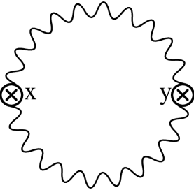
FIG. 2.: A graph with one hard loop

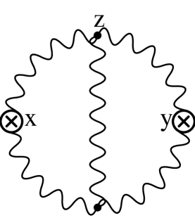
FIG. 3.: A graph with two hard loops

REFERENCES

- [1] P. Arnold, D. Son, L. Yaffe, Phys. Rev. D 55, 6264 (1997)
- [2] P. Huet, D.T. Son, Phys. Lett. B 393, 94 (1997).
- [3] K. Kajantie, K. Rummukainen, M. Shaposhnikov, Nucl. Phys. B 407, 356 (1993).
- [4] J. Ambjørn, A. Krasnitz, Phys. Lett. B 362, 97 (1995).
- [5] J. Smit, W.H. Tang, Nucl. Phys. B 482, 265 (1996)
- [6] G.D. Moore, N.G. Turok, “Lattice Chern-Simons Number Without Ultraviolet Problems,” Report No. PUPT-1681, hep-ph/9703266.
- [7] R.P Feynman, A.R. Hibbs, Quantum Mechanics and Path Integrals, Chapter 12 (McGraw-Hill, New York 1965).
- [8] E. Calzetta, B.L. Hu, Phys. Rev. D 49, 6636 (1994).
- [9] C. Greiner, B. Müller, Phys. Rev. D 55, 1026 (1997).
- [10] D. Bodeker, L. McLerran, A. Smilga, Phys. Rev. D 52 4675 (1995).
- [11] J-P. Blaizot, E. Iancu, Nucl. Phys. B 417, 608 (1997).
- [12] P.F. Kelly, Q. Liu, C. Lucchesi, C. Manuel, Phys. Rev. Lett. 72, 3461 (1994); Phys. Rev. D 50, 4209 (1994).
- [13] E.M. Lifshitz, L.P. Pitaevskii, Physical Kinetics (Pergamon Press, Oxford, 1981).
- [14] H. Risken, The Fokker-Planck Equation (Springer-Verlag, Berlin, 1989).
- [15] G. Aarts, J. Smit, Phys. Lett. B 393, 395 (1997).
- [16] P. Arnold, Phys. Rev. D 55 7781 (1997).
- [17] C.R. Hu, B. Muller, “Classical Lattice Gauge Fields with Hard Thermal Loops,” Report No. DUKE-TH-96-133, hep-ph/9611292.