Effective action and motion of a cosmic string

Abstract

We examine the leading order corrections to the Nambu effective action for the motion of a cosmic string, which appear at fourth order in the ratio of the width to radius of curvature of the string. We determine the numerical coefficients of these extrinsic curvature corrections, and derive the equations of motion of the worldsheet. Using these equations, we calculate the corrections to the motion of a collapsing loop, a travelling wave, and a helical breather. From the numerical coefficients we have calculated, we discuss whether the string motion can be labelled as ‘rigid’ or ‘antirigid,’ and hence whether cusp or kink formation might be suppressed or enhanced.

I Introduction

The study of topological or vacuum defects is of importance in many areas of contemporary physics. In high energy physics, a defect will generically occur during a symmetry breaking process where different parts of a medium choose different vacuum energy configurations, and the non-compatibility of these different vacua forces a sheet, line, or point of energy where these non-compatible vacua meet. The relevant vacuum order parameter then becomes indeterminate—this is the defect. A defect may be topological [5], in that it is the topology of the vacuum that simultaneously allows formation, and prevents dissipation, of these objects—but other types of defect are also possible. For instance, a defect may be stable dynamically (i.e. classically, due to energy considerations) but not topologically, as it happens for semilocal [6] or electroweak [7] defects. A defect can even be ‘topological’ and unstable, as in the case of textures [8], but nonetheless of physical importance.

In cosmology, there has been much speculation that topological defects (stable or otherwise) might have played an important role in structure formation [9]. In general, there are two main concerns when considering the cosmological effects of topological defects: their gravitational effects and their dynamics. Any theory concerning galaxy formation must be able to allow or constrain the presence of strongly self-gravitating objects. But the dynamics of the defects are in fact even more important, for it is the dynamics that determine to a large extent the shapes of the gravitating defects. For instance, if cosmic strings did not intercommute, any network would rapidly become tangled and would not obey a scaling law; such a configuration would be in conflict with the universe we see around us today. Even with intercommutation [10], strings which are strongly rigid and hence straight will have different gravitational effects to those that are very crinkly [11, 12].

The dynamical behaviour of a defect is generally assumed to be approximated by an effective action, a description which models the rather large numbers of degrees of freedom of the full field theory by the smaller number of degrees of freedom based on the position of the core of the defect. Attempts to derive effective actions or equations of motion for topological defects have commonly focussed on the strong coupling limit, meaning that of large values of the coupling coefficient $\lambda$ of the relevant Higgs field. In this limit, the defect becomes infinitesimally thin and effectively decouples from the other (infinitely massive) particles in the field theory. The study of the effective motion of topological defects has been extended [13, 14, 15] away from the limit $\lambda\rightarrow\infty$ to cases for which the thickness is small but not exactly zero. The resultant effective action generically contains a ‘zero-thickness’ term proportional to the area of the defect [16, 17], and extrinsic curvature terms which appear at quadratic order in the thickness [13, 14, 15]. The exact form of these second order terms is dependent on whether an ‘off-shell’ or ‘on-shell’ approach has been used to derive the effective action as was explained using the example of the domain wall in [18], and one finds that in a self-consistent order by order solution of the equations of motion, the only quadratic correction appearing is due to the geometry of the defect worldsurface, and is proportional to its intrinsic Ricci curvature [18]. For the domain wall, this term gives corrections to the motion, however for the string this term is a topological invariant—proportional to the Euler character of the worldsheet—and hence does not give any correction to the Nambu equations of motion.

The leading order corrections to the motion of a cosmic string were shown by one of us, [19], to appear at quartic order in the string width. In this paper, a systematic expansion of the geometry and field equations clarified an earlier discrepancy concerning second order ‘twist’ terms [13], and derived the fourth order action of the string, which is

$$S=-\mu\int d^{2}\sigma\sqrt{-\gamma}\bigg{[}1-r_{s}^{2}{\alpha_{1}\over\mu}{\cal R}+r_{s}^{4}\bigg{(}{\alpha_{2}\over\mu}{\cal R}^{2}+{\alpha_{3}\over\mu}{\cal K}_{{}_{i}\mu\nu}{\cal K}_{{}_{j}}^{\mu\nu}{\cal K}_{{}_{i}\lambda\rho}{\cal K}_{{}_{j}}^{\lambda\rho}\bigg{)}\bigg{]},$$ (1)

where ${\cal R}$, ${\cal K}_{{}_{i}\mu\nu}$ are the Ricci and extrinsic curvatures of the worldsheet (to be defined in the next section), and the $\alpha_{i}$ are numerical coefficients depending on the field theory modelling the vortex (to be defined in section III for the Abelian-Higgs model). Unlike the domain wall, whose background solution, and extrinsic curvature corrections can be expressed analytically [18], the prototypical cosmic string solution, the Nielsen–Olesen vortex [16], does not have a closed analytic form, hence these coefficients must be evaluated numerically.

As soon as one calculates corrections to the Nambu action, it becomes of general concern whether or not these corrections cause the motion of the defect to be ‘rigid’ or ‘antirigid.’ The implications of extrinsic curvature terms for string motion have been well-explored [14, 20, 21, 22, 23], however, it is not always easy to decide a priori (especially for the fourth order terms) whether the strings will be rigid or not, or indeed what one means by rigid [23].

In this paper we address these issues. We determine the numerical values of the $\alpha_{i}$ for the Abelian-Higgs model by solving the perturbed field equations for the non-flat worldsheet. We then derive the fourth order equations of motion from Anderson’s action and calculate corrections to three ‘test case’ trajectories: the circular loop, the travelling wave, and the helical breather. These three solutions display different characteristics which should be mirrored in the corrections to the Nambu motion if the rigidity of the string is to be determined. The loop collapses to a point [24], and rigidity would be indicated by a retardation of this collapse. A travelling wave on the other hand has been shown to be an exact solution of the full field theory [25], and should not exhibit any corrections if our approach is to be trusted. The helical breather (see e.g. [26]) is a time dependent solution which is never singular. Rigidity for this trajectory is more subtle, since the helical breather is never singular, however, we could call the string rigid if the tendency of the correction is to lower the magnitude of the scalar curvature of the worldsheet. As we will see, it is rather difficult to give an intuitive criterion for rigidity.

The layout of the paper is as follows. In the next section we review the formalism for the derivation of the effective action. In section III we rederive Anderson’s action, and present new numerical results evaluating the coefficients appearing in the action. In section IV we derive the equations of motion of the fourth order string, and in section V we calculate corrections to three test trajectories. In section VI we discuss the question of rigidity and conclude.

II Deriving the effective action

In this section we review the formalism required for the derivation of the string effective action. This formalism is largely based on the contents of [14, 19]. The problem of building the effective action is to reduce some four-dimensional field theoretic action integral

$$S=-\int d^{4}x\sqrt{-g}{\cal L}$$ (2)

to some two-dimensional worldsheet integral

$$S_{\rm eff}=-\int d^{2}\sigma\sqrt{-\gamma}{\cal L}_{\rm eff}.$$ (3)

We follow the canonical approach by setting up a coordinate system based on the worldsheet, and expanding the action and equations of motion around this worldsheet. By ‘expand’ we mean that we do not expect in one go to be able to solve the full equations of motion and integrate out (otherwise why find an effective action) but that we will be able to express the equations of motion for the system in terms of an expansion in $r_{s}\kappa$, where $r_{s}$ is the radius of the string, and $\kappa$ a typical scale of the extrinsic curvature of the worldsheet. We then solve the equations of motion in the directions perpendicular to the worldsheet, and integrate out the four-dimensional action (2) over these degrees of freedom to get an action of the form (3).

We will look at the particular case of a U(1) local string in flat spacetime (signature $+,-,-,-$). This is a vortex solution of the Abelian-Higgs model

$${\cal L}=\left({\cal D}_{\mu}\varphi\right)^{\dagger}\left({\cal D}^{\mu}\varphi\right)-{1\over 4}{\tilde{F}}^{\mu\nu}{\tilde{F}}_{\mu\nu}-{\lambda\over 4}(|\varphi|^{2}-\eta^{2})^{2},$$ (4)

where ${\cal D}_{\mu}=\nabla_{\mu}+ieA_{\mu}$ is the usual gauge covariant derivative, and ${\tilde{F}}_{\mu\nu}$ the field strength associated with $A_{\mu}$. We rewrite the field content of this model in the usual way:

$$\varphi(x^{\alpha}) = \eta\,X(x^{\alpha})e^{i\chi(x^{\alpha})}$$ (6)

$$A_{\mu}(x^{\alpha}) = \frac{1}{e}\,\bigg{[}P_{\mu}(x^{\alpha})-\nabla_{\mu}\chi(x^{\alpha})\bigg{]},$$ (7)

so that the vacuum is characterised by $X=1$. In terms of these new variables, the Lagrangian becomes

$${\cal L}=\eta^{2}(\nabla_{\mu}X)^{2}+\eta^{2}P_{\mu}^{2}X^{2}-\frac{1}{4e^{2}}F_{\mu\nu}^{2}-\frac{\lambda\eta^{4}}{4}(X^{2}-1)^{2},$$ (8)

where $F_{\mu\nu}$ is now the field strength of $P_{\nu}$. By making a compensating gauge transformation in $A_{\mu}$, we have absorbed the unphysical gauge degree of freedom of the theory. For future reference, here are the equations of motion for the new fields:

$$\frac{1}{\sqrt{-g}}\,\partial_{\mu}\sqrt{-g}\,\partial^{\mu}X = P_{\mu}P^{\mu}X-\frac{\lambda\eta^{2}}{2}X(X^{2}-1)$$ (10)

$$\frac{1}{\sqrt{-g}}\,\partial_{\mu}\sqrt{-g}\,F^{\mu\nu} = -2e^{2}\eta^{2}X^{2}P^{\nu}.$$ (11)

These equations are known to admit vortex solutions, the best known being that due to Nielsen and Olesen [16]—a solution corresponding to an infinite straight static string. A vortex solution is characterised by the fact that the scalar field phase has a non-zero winding number around an axis corresponding to the zeroes of the Higgs field (X=0). If we choose the string axis to be aligned with the $z$-axis, then a gauge can be chosen in which the vortex solution takes the form

$$\varphi=\eta\,X_{\rm NO}(\sqrt{\lambda}\eta\rho)e^{i\theta},\qquad A_{\mu}={1\over e}\left[P_{\rm NO}(\sqrt{\lambda}\eta\rho)-1\right]\nabla_{\mu}\theta$$ (12)

in cylindrical polar coordinates, where $X_{\rm NO}$ and $P_{\rm NO}$ satisfy the (generically) second order coupled differential equations:

$$-X^{\prime\prime}-{X^{\prime}\over r}+{XP^{2}\over r^{2}}+{1\over 2}X(X^{2}-1) = 0$$ (14)

$$-P^{\prime\prime}+{P^{\prime}\over r}+\beta PX^{2} = 0$$ (15)

and we have introduced the Bogomol’nyi parameter $\beta=2e^{2}/\lambda$. $\beta\to 0$ is the global string, and $\beta=1$ is the critical (supersymmetric) string for which the equations of motion factor to two coupled first order equations:

$$rX^{\prime} = XP,$$ (17)

$$P^{\prime} = \frac{1}{2}r\big{(}X^{2}-1\big{)}.$$ (18)

Intuitively we expect the solution for a general worldsheet to be very close to the Nielsen–Olesen solution in suitable coordinates, and that we might be able to expand the fields, and therefore the action, around this approximate solution. Let us now try to make this idea more concrete.

First we choose a worldsheet-based coordinate system. (Note this will only be valid within the radii of curvature of the worldsheet.) We start by coordinatising the worldsheet by $\sigma$ and $\tau$ as usual. Since we are in flat space, at each point on the worldsheet we have a well defined orthogonal flat two-plane, and such orthogonal planes do not intersect within the radii of curvature of the worldsheet. Thus we can thicken the worldsheet to a worldblanket by defining $\sigma$ and $\tau$ to be constant on such orthogonal planes. Since the worldsheet $\cal W$ has codimension 2, it has two associated families of unit normals $\{n_{{}_{i}}^{\mu}\}$. We choose a cartesian parametrisation of the orthogonal planes such that $\left({\partial\over\partial\xi^{i}}\right)^{\mu}_{\xi^{i}=0}=n_{{}_{i}}^{\mu}$. Thus $\{\tau,\sigma,\xi^{i}\}$ define a coordinate system in the vicinity of the worldsheet. In general it will not be possible to choose this system to be globally orthogonal, however, we will assume that the normal fields have been chosen so that the departure from orthogonality is minimal, i.e. of order of the extrinsic curvature of the worldsheet.

Because we no longer have a flat coordinate system, the connection will no longer be trivial, although the curvature components should still vanish. In order to examine the form of these relations, we use a Gauss–Codazzi approach [27] (see also [28] for more of a physicist’s approach). For shorthand we denote by $\{\sigma^{A}\}$ ($A=0,1$) the coordinates $\{\tau,\sigma\}$, the worldsheet by $\cal W$ and the Minkowski spacetime by $\cal M$.

The first fundamental form $h_{\mu\nu}$ of $\cal W$ is defined as

$$h_{\mu\nu}=g_{\mu\nu}+n_{{}_{i}\mu}\,n_{{}_{i}\nu}.$$ (19)

The tensor $h_{\mu\nu}$ acts as a projector onto $\cal W$, but is still a tensor in the 4-dimensional spacetime. For the metric intrinsic to the worldsheet, one uses the familiar

$$\gamma_{AB}={\partial X^{\mu}\over\partial\sigma^{A}}{\partial X_{\mu}\over\partial\sigma^{B}},$$ (20)

where $X^{\mu}(\sigma^{A})$ are the spacetime coordinates of the submanifold $\cal W$. This gives an interpretation of $\cal W$ as both a worldsheet in spacetime and a two-dimensional manifold with its own intrinsic geometry. One can define the intrinsic curvature of $\cal W$ in the standard way, and the extrinsic curvatures, or second fundamental forms, by

$${\cal K}_{{}_{i}\mu\nu}=h_{(\mu}^{\rho}h_{\nu)}^{\sigma}\nabla_{\rho}n_{{}_{i}\sigma}.$$ (21)

These extrinsic curvatures ${\cal K}_{{}_{i}\mu\nu}$ measure how $\cal W$ curves in $\cal M$. Since the codimension of the worldsheet is greater than one, we also have a non-trivial normal fundamental form

$${\tilde{\omega}}_{\mu}=\frac{1}{2}\varepsilon_{ij}n_{{}_{j}\nu}\nabla_{\mu}n_{{}_{i}}^{\nu},$$ (22)

where $\varepsilon_{ij}$ is the alternating symbol on two indices. This represents how near to orthogonality the worldblanket coordinate system is; it measures the rotation of the $n_{{}_{i}}^{\mu}$ in their own planes as one moves around the worldsheet. Note that, despite lying tangent to $\cal W$, $\tilde{\omega}_{\mu}$ is a gauge dependent object, depending on the choice of the normal fields—an SO(2) gauge group. In fact, $\tilde{\omega}_{\mu}$ is the connection on the normal bundle of $\cal W$.

Now, we may write

$$\nabla_{(\mu}n_{{}_{i}\nu)}={\cal K}_{{}_{i}\mu\nu}-\varepsilon_{ij}{\tilde{\omega}}_{(\mu}n_{{}_{j}\nu)},$$ (23)

where the symmetrization is understood to be only acting on indices of the same type, so that the ‘$j$’ above does not participate in any symmetrization. This now indicates an alternative definition of the second fundamental forms:

$${\cal K}_{{}_{i}\mu\nu}=\frac{1}{2}{\cal L}_{i}g_{\mu\nu}+\varepsilon_{ij}{\tilde{\omega}}_{(\mu}n_{{}_{j}\nu)}=\frac{1}{2}{\cal L}_{i}h_{\mu\nu}.$$ (24)

where ${\cal L}_{i}$ denotes the Lie derivative with respect to $n_{{}_{i}}^{\mu}$. We may now use the Riemann identity in flat space to derive the following relation for the extrinsic curvatures:

$$R_{\sigma(\mu\nu)\rho}n_{{}_{i}}^{\sigma}n_{{}_{j}}^{\rho}={\cal L}_{j}{\cal K}_{{}_{i}\mu\nu}-{\cal K}_{{}_{i}\rho(\mu}{\cal K}_{{}_{j}\nu)}^{\rho}=0.$$ (25)

Therefore, contracting with $g^{\mu\nu}$ gives

$${\cal L}_{j}{\cal K}_{{}_{i}}=-{\cal K}_{{}_{i}\mu\nu}{\cal K}_{{}_{j}}^{\mu\nu}$$ (26)

In addition, note that

$${\cal L}_{i}{\tilde{\omega}}_{\mu}=n_{{}_{i}}^{\nu}\nabla_{\nu}{\tilde{\omega}}_{\mu}+{\tilde{\omega}}_{\nu}\nabla_{\mu}n_{{}_{i}}^{\nu}={\frac{1}{2}}n_{{}_{i}}^{\nu}\nabla_{\nu}\left(\varepsilon_{jk}n_{{}_{k}\sigma}\nabla_{\mu}n_{{}_{j}}^{\sigma}\right)+{\tilde{\omega}}_{\nu}\nabla_{\mu}n_{{}_{i}}^{\nu}=0$$ (27)

and

$${\cal L}_{i}n_{{}_{j}\nu}=n_{{}_{j}\mu}\nabla_{\nu}n_{{}_{i}}^{\mu}={\tilde{\omega}}_{\nu}\varepsilon_{ij}.$$ (28)

The system of equations (24–28) give the ‘equations of motion’ for the geometry of the system, which together with (8) form the full equations of motion for the string.

In order to extract a low energy effective action, we will need to expand these quantities and equations of motion in terms of the thickness of the string, $r_{s}$. To do this systematically we define the dimensionless parameter $\epsilon$ by

$$\epsilon=\frac{\kappa}{{\sqrt{\lambda}}\eta}\propto\kappa r_{s}$$ (29)

where $\kappa^{-1}$ represents a typical radius of curvature of the worldsheet. We then define the zero thickness limit to mean $\epsilon\to 0$ with $\mu\propto\eta^{2}$, the energy per unit length of the string, fixed. Note that this may not necessarily mean that the string width is zero, since instead the extrinsic curvature could be zero (a flat worldsheet). However, if $\kappa\neq 0$, this limit corresponds to the conventional $\lambda\to\infty$ limit.

We now redefine coordinates so that the worldsheet has thickness and curvature of order unity by setting

$$x^{i} = \xi^{i}/r_{s}$$ (31)

$$s^{A} = \sigma^{A}\kappa$$ (32)

and redefining for consistency the following variables

$$K_{{}_{i}\mu\nu} = {\cal K}_{{}_{i}\mu\nu}/\kappa$$ (34)

$$\omega_{\mu} = {\tilde{\omega}}_{\mu}/\kappa$$ (35)

$${\hat{P}}_{\mu} = r_{s}P_{\mu}.$$ (36)

The worldsheet geometry equations (24–27) become

$${\cal L}_{i}h_{\mu\nu} = 2\epsilon K_{{}_{i}\mu\nu}$$ (38)

$${\cal L}_{i}g_{\mu\nu} = 2\epsilon[K_{{}_{i}\mu\nu}-\varepsilon_{ij}\omega_{(\mu}n_{{}_{j}\nu)}]$$ (39)

$${\cal L}_{j}K_{{}_{i}\mu\nu} = \epsilon K_{{}_{i}\sigma(\mu}K_{{}_{j}\nu)}^{\sigma}$$ (40)

$${\cal L}_{j}K_{{}_{i}} = -\epsilon K_{{}_{i}\mu\nu}K_{{}_{j}}^{\mu\nu}$$ (41)

$${\cal L}_{j}\omega_{\mu} = 0,$$ (42)

and the field equations (8) become:

$${1\over\sqrt{-g}} \bigg{\{}\partial_{i}\bigg{[}\sqrt{-g}\big{(}g^{ij}\partial_{j}X+\epsilon g^{iA}\partial_{A}X\big{)}+\epsilon\,\partial_{A}\big{(}\sqrt{-g}(g^{iA}\partial_{i}X+\epsilon g^{AB}\partial_{B}X)\big{)}\bigg{]}\bigg{\}}$$ (44)

$$={\hat{P}}_{\mu}{\hat{P}}_{\nu}g^{\mu\nu}X-{\frac{1}{2}}X(X^{2}-1)$$

$${1\over\sqrt{-g}} \mathchoice{{\hbox{\boldmath$\displaystyle\Bigg{(}$}}}{{\hbox{\boldmath$\textstyle\Bigg{(}$}}}{{\hbox{\boldmath$\scriptstyle\Bigg{(}$}}}{{\hbox{\boldmath$\scriptscriptstyle\Bigg{(}$}}}\partial_{i}\bigg{\{}\sqrt{-g}\bigg{[}g^{ik}g^{jl}{\hat{F}}_{kl}+(g^{iA}g^{jl}-g^{il}g^{jA})(\epsilon\partial_{A}{\hat{P}}_{l}-\partial_{l}{\hat{P}}_{A})+\epsilon g^{iA}g^{jB}{\hat{F}}_{AB}\bigg{]}\bigg{\}}+$$ (47)

$$\epsilon\,\partial_{A}\bigg{\{}\sqrt{-g}\bigg{[}g^{Ak}g^{jl}{\hat{F}}_{kl}+(g^{Ak}g^{jB}-g^{AB}g^{jk})(\partial_{k}{\hat{P}}_{B}-\epsilon\partial_{B}{\hat{P}}_{k})+\epsilon g^{AB}g^{jC}{\hat{F}}_{BC}\bigg{]}\bigg{\}}\mathchoice{{\hbox{\boldmath$\displaystyle\Bigg{)}$}}}{{\hbox{\boldmath$\textstyle\Bigg{)}$}}}{{\hbox{\boldmath$\scriptstyle\Bigg{)}$}}}{{\hbox{\boldmath$\scriptscriptstyle\Bigg{)}$}}}$$

$$=-\beta X^{2}(g^{ij}{\hat{P}}_{i}+g^{jA}{\hat{P}}_{A})$$

$${1\over\sqrt{-g}} \mathchoice{{\hbox{\boldmath$\displaystyle\Biggl{(}$}}}{{\hbox{\boldmath$\textstyle\Biggl{(}$}}}{{\hbox{\boldmath$\scriptstyle\Biggl{(}$}}}{{\hbox{\boldmath$\scriptscriptstyle\Biggl{(}$}}}\partial_{i}\bigg{\{}\sqrt{-g}\bigg{[}g^{ik}g^{Al}{\hat{F}}_{kl}+(g^{iB}g^{Al}-g^{il}g^{AB})(\epsilon\partial_{B}{\hat{P}}_{l}-\partial_{l}{\hat{P}}_{B})+\epsilon g^{iB}g^{AC}{\hat{F}}_{BC}\bigg{]}\bigg{\}}+$$ (50)

$$\epsilon\,\partial_{B}\bigg{\{}\sqrt{-g}\bigg{[}g^{Bk}g^{Al}{\hat{F}}_{kl}+(g^{BC}g^{Al}-g^{Bl}g^{AC})(\epsilon\partial_{C}{\hat{P}}_{l}-\partial_{l}{\hat{P}}_{C})+\epsilon g^{BC}g^{AD}{\hat{F}}_{CD}\bigg{]}\bigg{\}}\mathchoice{{\hbox{\boldmath$\displaystyle\Biggr{)}$}}}{{\hbox{\boldmath$\textstyle\Biggr{)}$}}}{{\hbox{\boldmath$\scriptstyle\Biggr{)}$}}}{{\hbox{\boldmath$\scriptscriptstyle\Biggr{)}$}}}$$

$$=-\beta X^{2}(g^{jA}{\hat{P}}_{j}+g^{AB}{\hat{P}}_{B}).$$

Here, $\hat{F}_{ij}$ is the tensor $F_{ij}$ defined in terms of the rescaled variables. Finally, we also need the explicit expansion of the Lagrangian

$${\cal L}=\lambda\eta^{4} \mathchoice{{\hbox{\boldmath$\displaystyle\Biggl{(}$}}}{{\hbox{\boldmath$\textstyle\Biggl{(}$}}}{{\hbox{\boldmath$\scriptstyle\Biggl{(}$}}}{{\hbox{\boldmath$\scriptscriptstyle\Biggl{(}$}}}\partial_{i}X\partial_{j}Xg^{ij}+2\epsilon\partial_{i}X\partial_{A}Xg^{iA}+\epsilon^{2}\partial_{A}X\partial_{B}Xg^{AB}+X^{2}{\hat{P}}_{\mu}{\hat{P}}_{\nu}g^{\mu\nu}-$$ (54)

$${1\over 2\beta}\bigg{\{}{\hat{F}}_{ij}\bigg{[}{\hat{F}}_{kl}g^{ik}g^{jl}+4(\partial_{k}{\hat{P}}_{A}-\epsilon\partial_{A}{\hat{P}}_{k})g^{ik}g^{jA}+2\epsilon{\hat{F}}_{AB}g^{iA}g^{jB}\bigg{]}+$$

$$\hskip 22.76219pt2(\partial_{i}{\hat{P}}_{A}-\epsilon\partial_{A}{\hat{P}}_{i})(\partial_{j}{\hat{P}}_{B}-\epsilon\partial_{B}{\hat{P}}_{j})(g^{ij}g^{AB}-g^{iB}g^{jA})+$$

$$\hskip 22.76219pt\epsilon{\hat{F}}_{AC}\bigg{[}4(\partial_{i}{\hat{P}}_{B}-\epsilon\partial_{B}{\hat{P}}_{i})g^{iA}g^{BC}+\epsilon{\hat{F}}_{BD}g^{AB}g^{CD}\bigg{]}\bigg{\}}-{\frac{1}{4}}(X^{2}-1)^{2}\mathchoice{{\hbox{\boldmath$\displaystyle\Bigg{)}$}}}{{\hbox{\boldmath$\textstyle\Bigg{)}$}}}{{\hbox{\boldmath$\scriptstyle\Bigg{)}$}}}{{\hbox{\boldmath$\scriptscriptstyle\Bigg{)}$}}}.$$

This now allows us to expand rigorously in powers of $\epsilon$. Note that so far we have made no assumptions about any of the fields or their dependence on the coordinates. We have simply rewritten the equations of motion, scaling with respect to the physical dimensionful quantities in the problem, leaving the equations of motion in terms of the dimensionless parameter $\epsilon$.

The procedure is as follows. We first consider the $\epsilon\to 0$ limit, with the metric and fundamental forms taking their geometrically defined values on the worldsheet. Since $\epsilon\to 0$ is also the flat worldsheet limit, we expect that the fields will take the Nielsen–Olesen form, which indeed turns out to be the case. In the next section we will go to higher orders in $\epsilon$, deriving the corrections to the geometry and fields, and hence the corresponding effective action. However, for the moment we conclude this section by proving that the Nielsen–Olesen solution is in fact the leading order behaviour for the vortex fields around the worldsheet.

To zeroth order

$${\cal L}_{i}h_{\mu\nu}={\cal L}_{i}g_{\mu\nu}={\cal L}_{i}K_{{}_{j}\mu\nu}=0,$$ (55)

hence all geometrical quantities take their worldsheet values, $K_{{}_{j}\mu\nu}(s^{A},x^{i})=K_{{}_{j}\mu\nu}(s^{A},0)$ etc. Hence

$$g_{{}_{0}\mu\nu}=\left({\matrix{\gamma_{AB}&0\cr 0&-\delta_{ij}\cr}}\right)$$ (56)

and thus the equations of motion for $X_{{}_{0}}$ and $P_{{}_{0}\mu}$ are

$$-\partial_{i}\partial_{i}X+({\hat{P}}_{i}^{2}-{\hat{P}}_{A}^{2})X+{\frac{1}{2}}X(X^{2}-1) =0$$ (58)

$$-\partial_{i}{\hat{F}}_{ij}+\beta X^{2}{\hat{P}}_{j} =0$$ (59)

$$-\partial_{i}\partial_{i}{\hat{P}}_{A}+\beta X^{2}{\hat{P}}_{A} =0.$$ (60)

These are solved by the Nielsen–Olesen solution, which is plotted in figure 1 against $r$ for $\beta=1$:

$$X_{{}_{0}}=X_{\rm NO}(r),\qquad{\hat{P}}_{{}_{0}j}=P_{\rm NO}(r)\partial_{j}\theta,\qquad{\hat{P}}_{{}_{0}A}=0.$$ (61)

Substitution of this solution back into (2) yields the familiar Nambu action. It is the corrections to this action we are interested in.

III The corrections to the Nambu action

We now derive the leading order corrections to the Nambu action. In order to calculate quantities away from the worldsheet, such as the metric, we must perform a Taylor expansion off the worldsheet

$$Q=Q|_{0}+\xi^{i}{\cal L}_{i}Q|_{0}+\frac{1}{2}\xi^{i}\xi^{j}{\cal L}_{i}{\cal L}_{j}Q|_{0}+\frac{1}{6}\xi^{i}\xi^{j}\xi^{k}{\cal L}_{i}{\cal L}_{j}{\cal L}_{k}Q|_{0}+\ldots$$ (62)

However, in calculating the Lie derivatives of the metric and its determinant some fortuitous cancellations occur. First note that

$${\cal L}_{k}{\cal L}_{j}K_{{}_{i}\mu\nu}=\epsilon{\cal L}_{k}\left(K_{{}_{i}\sigma(\mu}K_{{}_{j}\nu)\rho}g^{\sigma\rho}\right)=0$$ (63)

and also that

$${\cal L}_{k}{\cal L}_{j}{\cal L}_{i}\sqrt{-g}=\epsilon^{3}\sqrt{-g}\;\big{(} K_{{}_{i}}K_{{}_{j}}K_{{}_{k}}-K_{{}_{i}}K_{{}_{j}\nu}^{\mu}K_{{}_{k}\mu}^{\nu}-K_{j}K_{{}_{i}\nu}^{\mu}K_{{}_{k}\mu}^{\nu}-$$ (65)

$$K_{{}_{k}}K_{{}_{j}\nu}^{\mu}K_{{}_{i}\mu}^{\nu}+2K_{{}_{i}\sigma}^{\mu}K_{{}_{j}\mu}^{\nu}K_{{}_{k}\nu}^{\sigma}\big{)}=0,$$

which follows from a trace identity for the $2\times 2$ matrix $K$ [19]. Hence to all orders, the metric and the volume jacobian are given by

$$g_{\mu\nu} = g_{\mu\nu}|_{0}+2\epsilon x^{i}\left(K_{{}_{i}\mu\nu}|_{0}-\varepsilon_{ij}\omega_{(\mu}n_{{}_{j}\nu)}|_{0}\right)+\epsilon^{2}x^{i}x^{j}\left(K_{{}_{i}\sigma(\mu}|_{0}K_{{}_{j}\nu)}^{\sigma}|_{0}-\delta_{ij}\omega_{\mu}\omega_{\nu}\right)$$ (67)

$$\sqrt{-g} = \sqrt{-g}|_{0}\bigg{[}1+\epsilon x^{i}K_{{}_{i}}|_{0}+{\frac{1}{2}}\epsilon^{2}x^{i}x^{j}\left(K_{{}_{i}}|_{0}K_{{}_{j}}|_{0}-K_{{}_{i}AB}|_{0}K_{{}_{j}}^{AB}|_{0}\right)\bigg{]}.$$ (68)

This gives all the information on the geometrical contributions to the action. Now let us turn to the field theoretic contributions.

First note that since

$$\delta S|_{g_{{}_{0}\mu\nu}}=\int d^{2}\sigma d^{2}x\sqrt{-\gamma}\>\left({\delta S\over\delta X}\Big{|}_{g_{{}_{0}\mu\nu}}\hskip-5.69054pt\delta X+{\delta S\over\delta P_{\mu}}\Big{|}_{g_{{}_{0}\mu\nu}}\hskip-5.69054pt\delta P_{\mu}\right)$$ (69)

vanishes by the equations of motion, first order field corrections contribute at second order in the action, and second order corrections at fourth order.

To first order we may read off the equations for the corrections to the fields as

$$-\partial_{i}\partial_{i}X_{{}_{1}}-K_{{}_{i}}\partial_{i}X_{{}_{0}}+{\hat{P}}_{{}_{0}i}{\hat{P}}_{{}_{0}i}X_{{}_{1}}+2{\hat{P}}_{{}_{0}i}{\hat{P}}_{{}_{1}i}X_{{}_{0}}+{\frac{1}{2}}X_{{}_{1}}(3X_{{}_{0}}^{2}-1) = 0$$ (71)

$$-\partial_{i}{\hat{F}}_{{}_{1}ij}-K_{{}_{i}}{\hat{F}}_{{}_{0}ij}+\beta X_{{}_{0}}^{2}{\hat{P}}_{{}_{1}j}+2\beta X_{{}_{0}}X_{{}_{1}}{\hat{P}}_{{}_{0}j} = 0$$ (72)

$$-\partial_{i}(\omega_{A}x^{j}\varepsilon_{jk}{\hat{F}}_{ik})-\partial_{i}\partial_{i}{\hat{P}}_{{}_{1}A}+\beta X_{{}_{0}}^{2}{\hat{P}}_{{}_{1}A}+\beta X_{{}_{0}}^{2}\omega_{A}x^{j}\varepsilon_{jk}{\hat{P}}_{{}_{0}k} = 0.$$ (73)

The first two equations do not apparently lend themselves to a straightforward solution, however, we note that the equation of motion for the worldsheet obtained by varying the Nambu action is

$$\Box X^{\mu}=n_{{}_{i}}^{\mu}K_{i}=0,$$ (74)

which would indicate that the ‘driving’ terms in (71, 72) vanish and hence the appropriate solution is $X_{{}_{1}}=P_{{}_{1}j}=0$. Indeed, [14] demonstrated that unless the trace of the extrinsic curvature vanished on the defect, the first order perturbation equations have no solution that is regular and bounded. Thus in fact the appropriate solutions to the first two equations of (III) are $X_{1}=0$ and $P_{{}_{1}j}=0$.

The last equation of (III) is solved by [19]

$${\hat{P}}_{{}_{1}A}=-\omega_{A}x^{j}\varepsilon_{jk}{\hat{P}}_{{}_{0}k};$$ (75)

the presence of this term, as pointed out in [19], guarantees the gauge invariance of the effective action to worldsheet SO(2) gauge transformations, for on substituting in the form of the fields, this correction to ${\hat{P}}_{A}$ exactly cancels the ‘twist’ terms of Maeda and Turok, and we arrive at the second order result

$$S = -\mu\int d^{2}\sigma\sqrt{-\gamma}\;\left(1-\epsilon^{2}{\alpha_{1}\over\mu}K_{{}_{i}AB}^{2}\right)$$ (77)

$$= -\mu\int d^{2}\sigma\sqrt{-\gamma}\;\left(1-r_{s}^{2}{\alpha_{1}\over\mu}{\cal K}_{{}_{i}\mu\nu}^{2}\right),$$ (78)

where

$$\mu = 2\pi\eta^{2}\int_{0}^{\infty}rdr\hskip 1.70717pt\bigg{(}X_{{}_{0}}^{\prime 2}+{X_{{}_{0}}^{2}{\hat{P}}_{{}_{0}}^{2}\over r^{2}}+{{\hat{P}}_{{}_{0}}^{\prime 2}\over r^{2}\beta}+{\frac{1}{4}}(X_{{}_{0}}^{2}-1)^{2}\bigg{)}$$ (80)

$$\alpha_{1} = {\pi\eta^{2}\over 2}\int_{0}^{\infty}r^{3}dr\bigg{(}X_{{}_{0}}^{\prime 2}+{X_{{}_{0}}^{2}{\hat{P}}_{{}_{0}}^{2}\over r^{2}}+{{\hat{P}}_{{}_{0}}^{\prime 2}\over r^{2}\beta}+{\frac{1}{4}}(X_{{}_{0}}^{2}-1)^{2}\bigg{)}.$$ (81)

For the fourth order action we need the second order corrections to the fields, the volume factor already being exact to all orders. From (44–50) we may read off the equations for these as

$$-\partial_{i}\partial_{i}X_{{}_{2}}+x^{j}K_{{}_{i}AB}K_{{}_{j}}^{AB}\partial_{i}X_{{}_{0}}+{\hat{P}}_{{}_{0}i}{\hat{P}}_{{}_{0}i}X_{{}_{2}}+2{\hat{P}}_{{}_{0}i}{\hat{P}}_{{}_{2}i}X_{{}_{0}}+{\frac{1}{2}}X_{{}_{2}}(3X_{{}_{0}}^{2}-1) = 0$$ (83)

$$-\partial_{i}{\hat{F}}_{{}_{2}ij}+x^{k}K_{{}_{i}AB}K_{{}_{k}}^{AB}{\hat{F}}_{{}_{0}ij}+\beta X_{{}_{0}}^{2}{\hat{P}}_{{}_{2}j}+2\beta X_{{}_{0}}X_{{}_{2}}{\hat{P}}_{{}_{0}j} = 0$$ (84)

$$-\partial_{i}(\omega_{A}x^{j}\varepsilon_{jk}{\hat{F}}_{ik})-\partial_{i}\partial_{i}{\hat{P}}_{{}_{2}A} = 0.$$ (85)

To simplify these, and to remove the explicit $K$-dependence we will decompose in cylindrical harmonics by setting

$$X_{{}_{2}} = {\frac{1}{2}}gK_{{}_{i}AB}^{2}+{\bar{g}}x^{ij}K_{{}_{i}AB}K_{{}_{j}}^{AB}$$ (87)

$$P_{{}_{2}\phi} = {\frac{1}{2}}q_{\phi}K_{{}_{i}AB}^{2}+{\bar{q}_{\phi}}x^{ij}K_{{}_{i}AB}K_{{}_{j}}^{AB}$$ (88)

$$P_{{}_{2}r} = q_{r}\varepsilon_{ki}K_{{}_{k}AB}K_{{}_{j}}^{AB}x^{ij},$$ (89)

where

$$x^{ij}={x^{i}x^{j}\over r^{2}}-{\frac{1}{2}}\delta_{ij}.$$ (90)

This gives two sets of coupled second order differential equations

$$-g^{\prime\prime}-{g^{\prime}\over r}+{{\hat{P}}_{{}_{0}}^{2}g\over r^{2}}+{2{\hat{P}}_{{}_{0}}X_{{}_{0}}q_{\phi}\over r^{2}}+{\frac{1}{2}}g(3X_{{}_{0}}^{2}-1) = -rX_{{}_{0}}^{\prime}$$ (92)

$$-q_{\phi}^{\prime\prime}+{q_{\phi}^{\prime}\over r}+\beta X_{{}_{0}}^{2}q_{\phi}+2\beta X_{{}_{0}}{\hat{P}}_{{}_{0}}g = -r{\hat{P}}_{{}_{0}}^{\prime}$$ (93)

and

$$-{\bar{g}}^{\prime\prime}-{{\bar{g}}^{\prime}\over r}+{4{\bar{g}}\over r^{2}}+{{\hat{P}}_{{}_{0}}^{2}{\bar{g}}\over r^{2}}+{2{\hat{P}}_{{}_{0}}X_{{}_{0}}{\bar{q}_{\phi}}\over r^{2}}+{\frac{1}{2}}{\bar{g}}(3X_{{}_{0}}^{2}-1) = -rX_{{}_{0}}^{\prime}$$ (95)

$$-{\bar{q}_{\phi}}^{\prime\prime}+{{\bar{q}_{\phi}}^{\prime}\over r}+2q_{r}^{\prime}-{2q_{r}\over r}+\beta X_{{}_{0}}^{2}{\bar{q}_{\phi}}+2\beta X_{{}_{0}}{\hat{P}}_{{}_{0}}{\bar{g}} = -r{\hat{P}}_{{}_{0}}^{\prime}$$ (96)

$$4q_{r}-2{\bar{q}_{\phi}}^{\prime}+\beta r^{2}X_{{}_{0}}^{2}q_{r} = -r^{2}{\hat{P}}_{{}_{0}}^{\prime}.$$ (97)

There are no additional corrections to ${\hat{P}}_{A}$ at this level.

In the critical case $\beta=1$, the above equations reduce to two sets of first order ODE’s:

$$rg^{\prime} = X_{{}_{0}}q_{\phi}+\hat{P}_{{}_{0}}g,$$ (99)

$$\frac{q_{\phi}^{\prime}}{r} = X_{{}_{0}}g+\hat{P}_{{}_{0}}$$ (100)

and

$$r\bar{g}^{\prime} = X_{{}_{0}}\bar{q}_{\phi}+\hat{P}_{{}_{0}}\bar{g}+\frac{r\hat{P}_{{}_{0}}^{\prime}}{X_{{}_{0}}},$$ (102)

$$2\bar{g} = rq_{r}X_{{}_{0}}+\frac{r\hat{P}_{{}_{0}}^{\prime}}{X_{{}_{0}}},$$ (103)

$$2\bar{q}_{\phi}^{\prime}-4q_{r} = 2r\bar{g}X_{{}_{0}}.$$ (104)

Note that just as (III) is really two coupled second order ODE’s, (III) is really two coupled first order ODE’s. The fact that (90, III) reduce to such a first order form for $\beta=1$ is reassuring, since we do not expect to destroy supersymmetry simply by bending the string!

Substituting (III) into the action, and after some algebra, one arrives at Anderson’s result:

$$S = -\mu\int d^{2}\sigma\sqrt{-\gamma}\bigg{\{}1-\epsilon^{2}{\alpha_{1}\over\mu}K_{{}_{i}AB}^{2}+\epsilon^{4}\bigg{[}{\alpha_{2}\over\mu}(K_{{}_{i}AB}^{2})^{2}+{\alpha_{3}\over\mu}K_{{}_{i}AB}K_{{}_{j}}^{AB}K_{{}_{i}CD}K_{{}_{j}}^{CD}\bigg{]}\bigg{\}}$$ (106)

$$= -\mu\int d^{2}\sigma\sqrt{-\gamma}\bigg{\{}1-r_{s}^{2}{\alpha_{1}\over\mu}{\cal K}_{{}_{i}\mu\nu}^{2}\hskip 2.84526pt+r_{s}^{4}\bigg{[}{\alpha_{2}\over\mu}({\cal K}_{{}_{i}\mu\nu}^{2})^{2}+{\alpha_{3}\over\mu}{\cal K}_{{}_{i}\mu\nu}{\cal K}_{{}_{j}}^{\mu\nu}{\cal K}_{{}_{i}\lambda\rho}{\cal K}_{{}_{j}}^{\lambda\rho}\bigg{]}\bigg{\}},$$ (107)

where

$$\alpha_{2} = {\pi\eta^{2}\over 4}\int_{0}^{\infty}dr\bigg{[}r^{2}X_{{}_{0}}^{\prime}(2g-{\bar{g}})+{\hat{P}_{{}_{0}}^{\prime}\over\beta}(2q_{\phi}-{\bar{q}_{\phi}}-rq_{r})+{4r\hat{P}_{{}_{0}}^{2}\over\beta}\bigg{]}$$ (109)

$$\alpha_{3} = {\pi\eta^{2}\over 4}\int_{0}^{\infty}dr\bigg{[}2r^{2}X_{{}_{0}}^{\prime}{\bar{g}}+{2\hat{P}_{{}_{0}}^{\prime}\over\beta}({\bar{q}_{\phi}}+rq_{r})-{4r\hat{P}_{{}_{0}}^{2}\over\beta}\bigg{]}.$$ (110)

If $\beta=1$, it can be seen from (III, III) that $2\alpha_{2}+\alpha_{3}=0$.

To determine $\alpha_{2}$ and $\alpha_{3}$, we need to solve equations (90) and (III). This was done numerically by relaxation methods, using NAG routine D02GAF [29]. Sample solutions for both sets of equations for the critical case $\beta=1$ are plotted in figures 2 and 3. The first set of equations can be readily implemented and was solved by requiring that $g(0)=g(\infty)=q_{\phi}(0)=q_{\phi}(\infty)=0$. Before solving the second set of equations, we expressed $\bar{q}_{r}$ from (97) as:

$$q_{r}=\frac{2\bar{q}_{\phi}^{\prime}-r^{2}\hat{P}_{0}^{\prime}}{4+\beta r^{2}X_{0}^{2}}.$$ (111)

and eliminated it from the equations, which were then solved by asking that $\bar{g}(0)=\bar{g}(\infty)=\bar{q}_{\phi}^{\prime}(0)=\bar{q}_{\phi}(\infty)=0$. The solutions obtained clearly behave at the origin as:

$$g,\bar{g},q_{r} \sim r,$$ (113)

$$q_{\phi} \sim r^{2},$$ (114)

$$\bar{q}_{\phi} \sim \mathrm{const},$$ (115)

which can be checked to satisfy the asymptotic counterparts of (90, III).

We have computed the coefficients $\mu,\alpha_{1},\alpha_{2}$ and $\alpha_{3}$ for a range of values of $\beta$; the results are shown in figures 4–6 and in table I. The key points to note are that for the range of $\beta$ for which we computed the coefficients ($0<\beta\leq 100$) $\mu,\alpha_{1}>0$ and $\alpha_{3},\alpha_{2}+\alpha_{3}<0$; however, $2\alpha_{2}+\alpha_{3}$ is positive (negative) for $\beta<1$ ($\beta>1$) and $\alpha_{2}$ is positive for $\beta<\beta_{\mbox{crit}}\simeq 3.03$ and negative for $\beta>\beta_{\mbox{crit}}$.

IV The equations of motion for the string

In order to derive the equations of motion for the string we must express the action (III) in terms of the worldsheet coordinates, with respect to which we are varying the action. To do this, we note that

$$K_{{}_{i}AB}=n_{{}_{i}\mu},_{A}X^{\mu},_{B}=-n_{{}_{i}\mu}X^{\mu},_{AB}=-n_{{}_{i}\mu}X^{\mu}_{;AB}.$$ (116)

Hence, defining

$$N^{AB}_{CD}=X^{\mu;A}{}_{;C}X_{\mu;D}{}^{;B}$$ (117)

we see that

$$K_{{}_{i}AB}^{2} = -X^{\mu;AB}X_{\mu;AB}=-N^{AB}_{BA}$$ (119)

$$K_{{}_{i}AB}K_{{}_{j}}^{AB}K_{{}_{i}CD}K_{{}_{j}}^{CD} = X^{\mu;AB}X_{\mu;CD}X^{\nu;CD}X_{\nu;AB}=N^{AC}_{BD}N^{DB}_{CA}.$$ (120)

Now, the connection on the worldsheet is given by

$$\Gamma_{BC}^{A}={\frac{1}{2}}\gamma^{AE}\left(\gamma_{BE},_{C}+\gamma_{EC},_{B}-\gamma_{BC},_{E}\right)=\gamma^{AE}X^{\mu},_{E}{X_{\mu}},_{BC}$$ (121)

and the curvature (either directly or from the Gauss–Codazzi equations) is

$$R_{ABCD}=X^{\mu}_{;AC}X_{\mu;BD}-X^{\mu}_{;AD}X_{\mu;BC}.$$ (122)

We may therefore, using the identity

$$R_{ABCD}={\frac{1}{2}}R\left(\gamma_{AC}\gamma_{BD}-\gamma_{AD}\gamma_{BC}\right)$$ (123)

and the symmetries of $N$, infer the following useful relations:

$$R^{B}_{D} = {\frac{1}{2}}R\delta^{B}_{D}=-N^{AB}_{DA}$$ (125)

$$R = -N^{AB}_{BA}$$ (126)

$$N^{AC}_{BD}N^{DB}_{CA} = X^{\mu;AB}X_{\mu}^{\ ;CD}\left(R_{ACBD}+X^{\nu}_{;AD}X_{\nu;BC}\right)={\frac{1}{2}}R^{2}+N^{AD}_{BC}N^{CB}_{AD}.$$ (127)

We can now rewrite the action and its constituent variations as

$$S=-\mu\int d^{2}\sigma\sqrt{-\gamma}\;\bigg{\{}1-\epsilon^{2}{\alpha_{1}\over\mu}R+{\epsilon^{4}\over\mu}\bigg{[}(\alpha_{2}+{\frac{1}{2}}\alpha_{3})R^{2}+\alpha_{3}N^{AD}_{BC}N_{AD}^{CB}\bigg{]}\bigg{\}}$$ (128)

and

$$\delta\sqrt{-\gamma} = {\frac{1}{2}}\sqrt{-\gamma}\>\gamma^{AB}\delta\gamma_{AB}=\sqrt{-\gamma}\>\gamma^{AB}X^{\mu}_{\ ,A}\delta X_{\mu,B}$$ (130)

$$\delta R = -2X^{\mu;AB}\delta(X_{\mu;AB})+4N^{DA}_{AB}X^{\mu,B}\delta X_{\mu,D}=-2X^{\mu;AB}(\delta X_{\mu})_{;AB}-2RX^{\mu,D}\delta X_{\mu,D}$$ (131)

$$\delta\big{(}N^{AD}_{BC}N^{CB}_{AD}\big{)} = 4(\delta X_{\mu})_{;AB}X^{\mu;CD}N^{AB}_{CD}-4X^{\mu}_{\ ,F}\delta X_{\mu,A}\gamma^{AF}N^{ED}_{BC}N^{CB}_{ED}$$ (132)

[using the fact that $\delta\Gamma^{C}_{AB}X^{\mu}_{\ ,C}$ is parallel to the worldsheet whereas $X^{\mu;AB}$ is perpendicular, and (123).]

Noting that $\int\sqrt{-\gamma}R\propto\chi$, the Euler characteristic which is a topological invariant, or from the above equations, we see that the $\alpha_{1}$ term will not contribute to the equations of motion. The $R^{2}$ term, on the contrary, gives

$$3\big{(}\gamma^{AB}X^{\mu}_{\ ,A}R^{2}\big{)}_{;B}-4\left(RX^{\mu;AB}\right)_{;AB}=\left(X^{\mu,B}R^{2}-4R_{,A}X^{\mu;AB}\right)_{;B}=-4R_{;AB}X^{\mu;AB}$$ (133)

where we used the Riemann identity

$$(D_{A}D_{B}-D_{B}D_{A})X^{\mu}{}_{,C}=R_{CDAB}X^{\mu,D},$$ (134)

which implies

$$X^{\mu;AB}{}_{;B}=R^{AB}X^{\mu}_{\ ,B}={\frac{1}{2}}RX^{\mu,A}$$ (135)

at each step.

The $N^{2}$ term gives

$$3\left(X^{\mu,A}N^{ED}_{BC}N^{CB}_{ED}\right)_{;A}+4\left(N^{AB}_{CD}X^{\mu;CD}\right)_{;AB}\ ,$$

but

$$N^{AB}_{CD;A}X^{\mu;CD} = X^{\nu;B}{}_{;DA}X_{\nu;C}{}^{;A}X^{\mu;CD}$$ (136)

$$= {\frac{1}{2}}\left(X^{\nu}_{\ ;DA}X_{\nu;C}^{\ \ \ ;A}\right)_{;B}X^{\mu;CD}$$ (137)

$$= -{\frac{1}{4}}\left(R\gamma_{CD}\right)_{;B}X^{\mu;CD}=0,$$ (138)

hence the full equations of motion for the system are:

$$\frac{\mu}{\epsilon^{4}}\Box X^{\mu}=-(2\alpha_{3}+4\alpha_{2})R_{;AB}X^{\mu;AB}+3\alpha_{3}X^{\mu,A}\left(N^{ED}_{BC}N^{CB}_{ED}\right)_{;A}+4\alpha_{3}N^{AB}_{CD}X^{\mu;CD}{}_{;AB}.$$ (139)

It is possible to express these equations in terms of the extrinsic curvatures. Using (116) and

$$X^{\mu}_{;AB} = X^{\mu}_{,AB}-\Gamma^{C}_{AB}X^{\mu}_{,C}$$ (141)

$$X_{\mu,D}X^{\mu}{}_{;AB} = 0,$$ (142)

it follows that

$$X^{\mu}_{;AB} = \eta^{\mu\nu}X_{\nu;AB}=\left(\gamma^{CD}X^{\mu}_{,C}X^{\nu}_{,D}-\delta^{ij}n^{\mu}_{i}n^{\nu}_{j}\right)X_{\nu;AB}$$ (143)

$$= -\delta^{ij}n^{\mu}_{i}n^{\nu}_{j}X_{\nu,AB}=\delta^{ij}n^{\mu}_{i}K_{{}_{j}AB}.$$ (144)

Contracting the equation of motion with $n^{\mu}_{{}_{i}}$ and with $X^{\mu}_{,P}$ gives equations of motion normal and parallel to $\cal W$:

$$-\frac{\mu}{\epsilon^{4}}K^{A}_{{}_{i}A} = (4\alpha_{2}+2\alpha_{3})R_{;AB}K_{{}_{i}}^{AB}+4\alpha_{3}\delta^{jk}K_{{}_{j}}^{AC}K_{{}_{k}}^{BD}\;n^{\mu}_{{}_{i}}X_{\mu;CDAB}$$ (146)

$$0 = 3\alpha_{3}\left(N^{CD}_{EF}N^{FE}_{CD}\right)_{,P}+4\alpha_{3}N^{CD}_{EF}\gamma^{AE}\gamma^{BF}\;X^{\mu}_{,P}X_{\mu;CDAB}$$ (147)

Note that this latter equation (147) is an identity for the unperturbed worldsheet. We have verified that it does indeed hold using the lightcone gauge. Now,

$$n^{\mu}_{{}_{i}}X_{\mu;CDAB}= - K_{{}_{i}CD;AB}-\delta^{mn}\varepsilon_{im}\omega_{B}K_{{}_{n}CD;A}-\delta^{mn}\varepsilon_{im}\omega_{A}K_{{}_{n}CD;B}$$ (148)

$$- \delta^{mn}K_{{}_{m}CD}K^{E}_{{}_{n}A}K_{{}_{i}EB}-\delta^{mn}\varepsilon_{im}\omega_{A;B}K_{{}_{n}CD}+K_{{}_{i}CD}\omega_{A}\omega_{B},$$ (149)

which implies that the equations of motion also read:

$$\frac{\mu}{\epsilon^{4}}K^{A}_{{}_{i}A}=-(4\alpha_{2}+2\alpha_{3})R_{;AB}K_{{}_{i}}^{AB}+4\alpha_{3}K_{{}_{j}}^{AC}K_{{}_{j}}^{BD}\big{(} - K_{{}_{i}CD;AB}-\varepsilon_{ik}\omega_{B}K_{{}_{k}CD;A}-\varepsilon_{ik}\omega_{A}K_{{}_{k}CD;B}$$ (150)

$$- K_{{}_{k}CD}K^{E}_{{}_{k}A}K_{{}_{i}EB}-\varepsilon_{ik}\omega_{A;B}K_{{}_{k}CD}+K_{{}_{i}CD}\omega_{A}\omega_{B}\big{)}.$$ (151)

V Corrections to the motion of test trajectories

We now wish to derive the corrections to the motion of three test trajectories: the circular loop, the travelling wave, and the helical breather. We have chosen these three examples because they provide three different ways in which to observe the rigidity or otherwise of the string.

The loop trajectory is given by

$$X^{\mu}(\tau,\sigma)=\left(\tau,\cos\tau\cos\sigma,\cos\tau\sin\sigma,0\right),$$ (152)

and collapses to a point after a time period $\Delta\tau=\pi/2=L/4$, where $L=\oint d\sigma=2\pi$ is the length of the closed string. The extrinsic curvature invariants become singular at this point, hence rigidity would be indicated by a retardation of the collapse or a positive correction to the amplitude of the loop.

A travelling wave on the other hand is a variant of the flat worldsheet where a deformation of arbitrary size and form is introduced, the only constraint being that the deformation is a function of only one of the lightcone coordinates, $\sigma_{\pm}=\sigma\pm\tau$:

$$X^{\mu}(\tau,\sigma)=\left(\tau,f(\tau-\sigma),g(\tau-\sigma),\sigma\right)$$ (153)

This has been shown to be a solution of the full field theory [25], hence no correction should be found for this trajectory.

The helical breather is a time-dependent solution which may be written as

$$X^{\mu}(\tau,\sigma)=\left(\tau,\sqrt{1-q^{2}}\cos\tau\cos\sigma,\sqrt{1-q^{2}}\cos\tau\sin\sigma,q\sigma\right)$$ (154)

The limit $q\to 1$ corresponds to the flat worldsheet and the limit $q\to 0$ to the collapsing circular loop. For intermediate $q$ the trajectory is never singular, and the extrinsic curvature peaks at approximately $q^{-2}\sqrt{1-q^{2}}$. Rigidity would be indicated by a preference for lower extrinsic curvature and hence a negative correction to the amplitude of oscillation.

A Corrections to the motion of a collapsing loop

As a first example of the effects of curvature terms on the motion of freely-moving cosmic strings, we consider the collapse of a circular loop. In Cartesian coordinates, the position of this string is given by

$$X^{\mu}(\tau,\sigma)=\left(\tau,Z(\tau)\cos\sigma,Z(\tau)\sin\sigma,0\right),$$ (155)

and the normals to the worldsheet are

$$n_{{}_{2}}^{\mu} = \left(\dot{Z},\cos\sigma,\sin\sigma,0\right)/\sqrt{1-\dot{Z}^{2}}$$ (157)

$$n_{{}_{3}}^{\mu} = \left(0,0,0,1\right).$$ (158)

In this case, one obtains $\omega_{A}=0$, and

$${\cal K}_{{}_{2}AB} = \left(\begin{array}[]{c c}\ddot{Z}&0\\ 0&-Z\end{array}\right)/\sqrt{1-\dot{Z}^{2}}$$ (162)

$${\cal K}_{{}_{3}AB} = 0$$ (163)

$$\gamma_{AB} = \left(\begin{array}[]{c c}1-\dot{Z}^{2}&0\\ 0&-Z^{2}\end{array}\right)$$ (166)

$$\Gamma^{\tau}_{AB} = \left(\begin{array}[]{c c}\frac{-\dot{Z}\ddot{Z}}{1-\dot{Z}^{2}}&0\\ 0&\frac{Z\dot{Z}}{1-\dot{Z}^{2}}\end{array}\right)$$ (169)

$$\Gamma^{\sigma}_{AB} = \frac{\dot{Z}}{Z}\left(\begin{array}[]{c c}0&1\\ 1&0\end{array}\right).$$ (172)

The equation of motion to zeroth order is

$${\cal K}^{A}_{{}_{2}A}={Z\ddot{Z}+1-\dot{Z}^{2}\over Z(1-{\dot{Z}}^{2})^{3/2}}=0,$$ (173)

The general solution to this equation is $Z(\tau)=k\cos([\tau-\tau_{0}]/k)$. Choosing $k=1,\tau_{0}=0$ as initial conditions one obtains the canonical form of the loop trajectory (152). Note that for this choice of loop length $\kappa=1$ and we can use $K$ or ${\cal K}$ interchangeably.

We now wish to find the corrected solution to order $\epsilon^{4}=r_{s}^{4}$. To do this, we use equation (151) (technically its unrescaled counterpart). Since $K_{{}_{3}AB}$ and $\omega^{A}$ vanish, the RHS of (151) considerably simplifies to

$$4(\alpha_{2}+\alpha_{3}){\cal R}_{;AB}{\cal K}^{AB}=32(\alpha_{2}+\alpha_{3})\,\sec^{8}(\tau)\big{(}7\sec^{2}(\tau)-6\big{)}.$$ (174)

(Note that we have dropped the subscript ‘2’ on the extrinsic curvature.)

The left-hand side is obtained by varying the trace of ${\cal K}_{{}_{2}}$ from (173), whereby we obtain the equation for $\delta Z$ as

$$\delta\ddot{Z}+2\tan(\tau)\delta\dot{Z}-\delta Z=32\frac{r_{s}^{4}}{\mu}\left(\alpha_{2}+\alpha_{3}\right)\sec^{5}(\tau)\left(7\sec^{2}(\tau)-6\right).$$ (175)

The solution to this, with initial conditions $\delta Z(0)={\dot{\delta Z}}(0)=0$ is

$$\delta Z(\tau)=32\frac{\epsilon^{4}}{\mu}(\alpha_{2}+\alpha_{3})\bigg{(}\frac{7}{40}\sec^{5}(\tau)+\frac{1}{60}\sec^{3}(\tau)+\frac{1}{15}\sec(\tau)-\frac{31}{120}\cos(\tau)-\frac{\tau}{8}\sin(\tau)\bigg{)}.$$ (176)

Thus, the sign of $\alpha_{2}+\alpha_{3}$ determines whether the string is rigid or antirigid. This ‘loop rigidity parameter’ is plotted against $\beta$ on figure 7, and its negativity means that the loop is antirigid and tends to collapse faster than in the Nambu approximation. This is illustrated on figure 8, where we compare the zero-order solution $Z(\tau)=\cos(\tau)$ with the corrected solution $Z(\tau)=\cos(\tau)+\delta Z(\tau)$.

Note that the approximation breaks down when $|{\cal K}^{A}_{B}|=O(r_{s}^{-1})$, i.e. when $\cos(\tau)=O(r_{s})$. For example, in the illustration of collapse in figure 8, $r_{s}=1/10$ is rather large; we would hope that our approximation would be valid until the radii of curvature of the worldsheet became close to 1/10, let us say twice the radius of the string: 1/5. Inputting $|{\cal K}^{A}_{B}|=1/5$ gives $\tau\simeq 1.1$, which does indeed correspond to the point at which the solutions start to significantly differ in figure 8.

B The motion of a travelling wave

Now consider a travelling wave, whose position and normals are given by:

$$X^{\mu}(\tau,\sigma) = \left(\tau,f(\tau-\sigma),g(\tau-\sigma),\sigma\right)$$ (178)

$$n_{{}_{2}}^{\mu}\equiv n^{\mu} = \left(0,g^{\prime},-f^{\prime},0\right)/\sqrt{f^{\prime}{}^{2}+g^{\prime}{}^{2}}$$ (179)

$$n_{{}_{3}}^{\mu}\equiv m^{\mu} = \left(f^{\prime}{}^{2}+g^{\prime}{}^{2},f^{\prime},g^{\prime},f^{\prime}{}^{2}+g^{\prime}{}^{2}\right)/\sqrt{f^{\prime}{}^{2}+g^{\prime}{}^{2}},$$ (180)

where a prime denotes differentiation with respect to the argument, namely $\tau-\sigma$.

Writing

$$\lambda(\tau-\sigma) = f^{\prime}{}^{2}+g^{\prime}{}^{2}$$ (182)

$$\zeta(\tau-\sigma) = \left(f^{\prime\prime}g^{\prime}-f^{\prime}g^{\prime\prime}\right)/\lambda$$ (183)

$$\kappa_{2}(\tau-\sigma) = \left(f^{\prime\prime}g^{\prime}-f^{\prime}g^{\prime\prime}\right)/\sqrt{\lambda}$$ (184)

$$\kappa_{3}(\tau-\sigma) = \left(f^{\prime}f^{\prime\prime}+g^{\prime}g^{\prime\prime}\right)/\sqrt{\lambda},$$ (185)

one has:

$$\omega_{A} = \zeta\left(\begin{array}[]{c}1\\ -1\\ \end{array}\right)$$ (189)

$$K_{{}_{i}AB} = \kappa_{i}\left(\begin{array}[]{c c}1&-1\\ -1&1\\ \end{array}\right)$$ (192)

$$\gamma_{AB} = \left(\begin{array}[]{c c}1-\lambda&\lambda\\ \lambda&-1-\lambda\\ \end{array}\right)$$ (195)

$$\Gamma^{A}_{BC} = \frac{\lambda^{\prime}}{2}\left(\begin{array}[]{c}1\\ -1\\ \end{array}\right)\otimes\left(\begin{array}[]{c c}-1&1\\ 1&-1\\ \end{array}\right).$$ (200)

It is then straightforward to see that all terms on the right-hand side of (151) vanish separately, as do the traces of the extrinsic curvatures: the travelling wave is an exact solution to (at least) fourth order.

C Corrections to the motion of a helical string in breathing mode

We now consider the string given by the following position functions:

$$X^{\mu} = \left(\tau,Z(\tau)\cos(\sigma),Z(\tau)\sin(\sigma),q\sigma\right)$$ (202)

$$n_{{}_{2}}^{\mu} = \left(0,q\sin(\sigma),-q\cos(\sigma),Z\right)/\sqrt{q^{2}+Z^{2}}$$ (203)

$$n_{{}_{3}}^{\mu} = \left(\dot{Z},\cos(\sigma),\sin(\sigma),0\right)/\sqrt{1-\dot{Z}^{2}}.$$ (204)

This string is helical with breathing $q$: the limits $q\to 0$ and $q\to 1$ represent a collapsing loop and a straight string, respectively. [Note how (202–204) reduce to (155–155), and how all pertinent quantities in the equations of motion are obtained from these expressions.]

With this choice of normals, the fundamental forms are:

$$\gamma_{AB} = \left(\begin{array}[]{cc}1-\dot{Z}^{2}&0\\ 0&-(q^{2}+Z^{2})\\ \end{array}\right)$$ (208)

$$K_{{}_{2}AB} = -\frac{q\dot{Z}}{\sqrt{q^{2}+Z^{2}}}\left(\begin{array}[]{cc}0&1\\ 1&0\\ \end{array}\right)$$ (211)

$$K_{{}_{3}AB} = \frac{1}{\sqrt{1-\dot{Z}^{2}}}\left(\begin{array}[]{cc}\ddot{Z}&0\\ 0&-Z\\ \end{array}\right)$$ (214)

$$\omega_{A} = \frac{-q}{\sqrt{1-\dot{Z}^{2}}\sqrt{q^{2}+Z^{2}}}\left(\begin{array}[]{c}0\\ 1\\ \end{array}\right).$$ (217)

Hence the equations of motion to zeroth order become

$${\ddot{Z}\over(1-{\dot{Z}}^{2})^{3/2}}+\frac{Z}{(q^{2}+Z^{2})(1-{\dot{Z}}^{2})^{1/2}}=0.$$ (218)

This equation admits for general solution

$$Z(\tau)=\sqrt{k^{2}-q^{2}}\cos\left(\frac{\tau-\tau_{0}}{k}\right),$$ (219)

so that, choosing again the initial conditions $k=1,\tau_{0}=0$ and calling

$$\Omega(\tau)=\cos^{2}(\tau)+q^{2}\sin^{2}(\tau),$$ (220)

we have

$$\gamma_{AB} = \Omega\left(\begin{array}[]{c c}1&0\\ 0&-1\end{array}\right)$$ (224)

$$K_{{}_{2}AB} = q\sqrt{\frac{1-q^{2}}{\Omega}}\sin(\tau)\left(\begin{array}[]{c c}0&1\\ 1&0\\ \end{array}\right)$$ (227)

$$K_{{}_{3}AB} = -\sqrt{\frac{1-q^{2}}{\Omega}}\cos(\tau)\left(\begin{array}[]{c c}1&0\\ 0&1\\ \end{array}\right)$$ (230)

$$\omega_{A} = -\frac{q}{\Omega}\left(\begin{array}[]{c}0\\ 1\\ \end{array}\right).$$ (233)

The right-hand side of the corrected equation of motion becomes then

$$-32\epsilon^{4}\sqrt{1-q^{2}}\;\cos(\tau)\Omega^{-9/2}\left(\beta_{1}-\beta_{2}\Omega^{-1}+\beta_{3}\Omega^{-2}-\beta_{4}\Omega^{-3}\right),$$

where

$$\beta_{1} = 6\left[(\alpha_{2}+\alpha_{3})+\alpha_{2}q^{2}\right]$$ (235)

$$\beta_{2} = 7(\alpha_{2}+\alpha_{3})+(38\alpha_{2}+22\alpha_{3})q^{2}+(7\alpha_{2}-3\alpha_{3})q^{4}$$ (236)

$$\beta_{3} = 5q^{2}\left[(7\alpha_{2}+5\alpha_{3})+(7\alpha_{2}+2\alpha_{3})q^{2}\right]$$ (237)

$$\beta_{4} = 15q^{4}(2\alpha_{2}+\alpha_{3}),$$ (238)

and the left-hand side is obtained as before by varying the trace of $K_{{}_{3}}$:

$$\delta\left(K^{A}_{{}_{3}A}\right)=\Omega^{-3/2}\delta\ddot{Z}+2\Omega^{-5/2}(1-q^{2})\sin(\tau)\cos(\tau)\delta\dot{Z}+\Omega^{-5/2}\left[q^{2}-(1-q^{2})\cos^{2}(\tau)\right]\delta Z.$$ (239)

Finally, the corrected equations of motion are:

$$\delta\ddot{Z} + 2\frac{1-q^{2}}{\Omega}\sin(\tau)\cos(\tau)\delta\dot{Z}+\frac{q^{2}-(1-q^{2})\cos^{2}(\tau)}{\Omega}\delta Z$$ (240)

$$= -32\frac{\epsilon^{4}}{\mu}\sqrt{1-q^{2}}\cos(\tau)\Omega^{-3}\big{(}\beta_{1}-\beta_{2}\Omega^{-1}+\beta_{3}\Omega^{-2}-\beta_{4}\Omega^{-3}\big{)}.$$ (241)

Although it is possible to find an exact solution to this equation (see appendix for details), it is more instructive to consider the quasiflat limit $q\to 1$. In this case, equation (241) becomes

$$\delta\ddot{Z}+\delta Z=-32\frac{\epsilon^{4}\Delta^{3}}{\mu}\big{[}(\alpha_{2}+\alpha_{3})\cos(\tau)-(2\alpha_{2}+\alpha_{3})\cos(\tau)\sin^{2}(\tau)\big{]},$$ (242)

where $\Delta$ is defined by

$$q^{2}=1-\Delta^{2}.$$ (243)

The solution $\delta Z(\tau)$ satisfying $\delta Z(0)=\delta\dot{Z}(0)=0$ is then found to be

$$\delta Z=-\frac{\epsilon^{4}\Delta^{3}}{\mu}\bigg{[}4\left(2\alpha_{2}+3\alpha_{3}\right)\tau\sin(\tau)\\ +(2\alpha_{2}+\alpha_{3})\big{(}\cos\tau-\cos(3\tau)\big{)}\bigg{]}$$ (244)

The corrected trajectory can then be written:

$$Z+\delta Z=\Delta\left[1-\frac{\epsilon^{4}\Delta^{2}}{\mu}(2\alpha_{2}+\alpha_{3})\right]\cos\left\{\left[1+\frac{4\epsilon^{4}\Delta^{2}}{\mu}(2\alpha_{2}+3\alpha_{3})\right]\tau\right\}+\frac{\epsilon^{4}\Delta^{3}}{\mu}(2\alpha_{2}+\alpha_{3})\cos(3\tau)+\mbox{O}(\epsilon^{8}).$$ (245)

The effect of the correction is threefold: First, it alters the frequency of the motion, $\tau\to\left[1+4\epsilon^{4}\Delta^{2}(2\alpha_{2}+3\alpha_{3})/\mu\right]\tau$; since $(\alpha_{2}+\alpha_{3}),\alpha_{3}<0$ this has the effect of reducing the frequency—a tendency we would be tempted to call rigid. Secondly, the amplitude of the oscillation is altered by a factor $1-\epsilon^{4}\Delta^{2}(2\alpha_{2}+\alpha_{3})/\mu$. This could be either a amplification or reduction, depending on whether $\beta>1$ or $\beta<1$. Finally, a higher frequency oscillation is superposed on the motion for $\beta\neq 1$. If, for simplicity, we take $\beta=1$, so $2\alpha_{2}+\alpha_{3}=0$, we see that

$$Z+\delta Z=\Delta\cos\left[\left(1+\frac{8\epsilon^{4}\Delta^{2}}{\mu}\alpha_{3}\right)\tau\right]$$ (246)

i.e. the only effect of the correction is to reduce the frequency of oscillation of the breather, which would seem to be unambiguously rigid.

However, we now observe a curious property: Suppose instead we consider initialising the correction at the instant of maximal velocity: $\delta Z(-\pi/2)=\delta\dot{Z}(-\pi/2)=0$, we find

$$Z+\delta Z=\Delta\left[1-\frac{\epsilon^{4}\Delta^{2}}{\mu}(2\alpha_{2}+9\alpha_{3})\right]\sin\left\{\left[1+\frac{4\epsilon^{4}\Delta^{2}}{\mu}(2\alpha_{2}+3\alpha_{3})\right]\tau^{\prime}\right\}-\frac{\epsilon^{4}\Delta^{3}}{\mu}(2\alpha_{2}+\alpha_{3})\sin(3\tau^{\prime})+\mbox{O}(\epsilon^{8})$$ (247)

(where $\tau^{\prime}=\tau+\pi/2$). Now note that while the frequency of oscillation is decreased by the same amount, and the higher frequency term is still the same, the amplitude is now uniformly increased for all $\beta$. If, as before, we take $\beta=1$, we now find

$$Z+\delta Z=\Delta\left(1-\frac{8\epsilon^{4}\Delta^{2}}{\mu}\alpha_{3}\right)\sin\left[\left(1+\frac{8\epsilon^{4}\Delta^{2}}{\mu}\alpha_{3}\right)\tau^{\prime}\right],$$ (248)

in other words an increase in the amplitude of oscillation accompanies a similar decrease in its frequency. One cannot immediately see from this solution whether or not the behaviour is rigid, however, an analysis of the Ricci curvature near $\tau^{\prime}=0$ shows that it is in fact increased—a behaviour consistent with antirigidity! A calculation of the dependence of the curvature on general $q$ is presented in the appendix. The algebra is more complicated but the results are the same: all helical breathers display both rigid and antirigid characteristics.

The results of our helical breather calculations therefore appear rather ambiguous. If we wish to identify rigidity by the behaviour of a corrected trajectory—whether it increases or decreases curvature—we are forced to calculate the effect on the curvature (see appendix) and then the results appear to depend on the initial conditions. What this shows is that the ‘decrease in curvature’ criterion for rigidity is too naïve to be reliably applied in all situations.

VI The question of rigidity

We now want to determine whether a string can be labelled ‘rigid’ or ‘antirigid’. To do this, we use an argument based in that of Polyakov [21], which consists in determining how the action varies under a rescaling of the spacetime coordinates $X^{\mu}\to\lambda X^{\mu}$. Such transformations alter the scale of crinkles of the worldsheet and magnify or reduce small-scale structure, hence rigidity would be indicated by a extremum of the energy or the action with respect to the rescaling parameter $\lambda$, as illustrated in figure 11.

Out starting point is the action (III), which can be written

$$-S=\mu\int d^{2}\sigma\sqrt{-\gamma}-\epsilon^{2}\alpha_{1}\int d^{2}\sigma\sqrt{-\gamma}\>M_{ii}+\epsilon^{4}\alpha_{2}\int d^{2}\sigma\sqrt{-\gamma}\>M^{2}_{ii}+\epsilon^{4}\alpha_{3}\int d^{2}\sigma\sqrt{-\gamma}\>M_{ij}M_{ij},$$ (249)

where the matrix $M_{ij}$ is defined as

$$M_{ij}=K_{{}_{i}AB}K_{{}_{j}}^{AB}.$$ (250)

As $M_{ij}M_{ij}=M_{ii}^{2}-2\,\det(M)$, this can be expressed as

$$-S=\mu A-\epsilon^{2}\alpha_{1}\chi+\epsilon^{4}\big{[}(\alpha_{2}+\alpha_{3})I_{1}-2\alpha_{3}I_{2}\big{]},$$ (251)

with $A$ the area of the worldsheet for the range of $\{\tau,\sigma\}$ being integrated over and $\chi$ proportional to the Euler character of $\cal W$. Also,

$$I_{1} = \int d^{2}\sigma\sqrt{-\gamma}\>M^{2}_{ii},$$ (253)

$$I_{2} = \int d^{2}\sigma\sqrt{-\gamma}\>\det(M).$$ (254)

We now rescale $X^{\mu}\to\lambda X^{\mu}$, so that for $\lambda>1$ the worldsheet is expanded and for $\lambda<1$ it is shrunk. Then,

$$\gamma_{AB} \to \lambda^{2}\gamma_{AB},$$ (256)

$$K_{{}_{i}AB} \to \lambda K_{{}_{i}AB},$$ (257)

and thus $I_{i}\to\lambda^{-2}I_{i}$, $i=1,2$. The shape of the curve $S(\lambda)$ now depends explicitly on the integrals $I_{i}$, since $-S$ is rescaled as

$$-S\to\lambda^{2}\mu A+\epsilon^{2}\alpha_{1}\chi+\lambda^{-2}\epsilon^{4}\big{[}(\alpha_{2}+\alpha_{3})I_{1}-2\alpha_{3}I_{2}\big{]}.$$ (258)

We know that $\alpha_{3},\alpha_{2}+\alpha_{3}<0$, and clearly $I_{1}>0$, so in order to determine the shape of $S(\lambda)$ we only need to determine the sign of $\det(M)$. For these purposes, we can work in the conformal gauge, $\gamma_{AB}=\eta_{AB}$, and we find

$$\det(M)=\big{(}K_{{}_{2}00}K_{{}_{3}11}-K_{{}_{3}00}K_{{}_{2}11}\big{)}^{2}-2\big{(}K_{{}_{2}11}K_{{}_{3}10}-K_{{}_{3}11}K_{{}_{2}10}\big{)}^{2}\\ -2\big{(}K_{{}_{2}00}K_{{}_{3}10}-K_{{}_{3}00}K_{{}_{2}10}\big{)}^{2}.$$ (259)

If we impose the Nambu equations of motion, $K^{A}_{{}_{i}A}=0$, this determinant is strictly negative. Hence, since $\mu A$ is positive, we see that $S(\lambda)$ is unbounded, because the the coefficients multiplying $\lambda^{2}$ and $\lambda^{-2}$ have opposite signs.

We must therefore conclude that the string is antirigid. This does not mean that all the trajectories of the string exhibit antirigidity, but rather that it is impossible for all trajectories to be rigid.

Let us illustrate this by considering the trajectories of the previous section. For the collapsing loop, $\det(M)=0$, and as we noticed, $\alpha_{2}+\alpha_{3}$ determines alone the shape of $S(\lambda)$. This simplification came from the fact that the loop is flat, and therefore has only one nonvanishing extrinsic curvature.

For the travelling wave, $M_{ij}\equiv 0$, which is consistent with our observation of no corrections to this trajectory.

In the case of the helical breather, both $M_{ii}$ and $\det(M)$ are non-zero, so we do not expect results to depend on $\alpha_{2}+\alpha_{3}$. Even though the action is unstable to the scaling of the worldsheet, what is happening with the helical breather is that the correction does not always have a non-zero projection on this unstable mode. However, we would expect a general correction of the breather to exhibit an instability.

To sum up: We have reviewed the derivation of the effective action for a U(1) local cosmic string to fourth order in the ratio of string width to worldsheet curvature. We presented numerical results calculating the coefficients of these fourth order terms. We then derived the equations of motion for the string to fourth order, and calculated corrections to a sample of well-known trajectories. We have given a general argument for antirigidity of the cosmic string to fourth order, however by reference to our examples have shown that not all trajectories need behave in an ‘antirigid’ fashion—rigidity it appears is rather like a theorem, it may work in special cases, but one needs only find a single counterexample to disprove it.

The Helical Breather

Recall from section V C that the helical breather solution to the Nambu action is

$$X^{\mu}=\big{(}\tau,\Delta\cos(\tau)\cos(\sigma),\Delta\cos(\tau)\sin(\sigma),q\sigma\big{)}$$ (260)

[where $\Delta$ is defined in (243)] and that the equation of motion for $\delta Z(\tau)$ is (241):

$$\delta\ddot{Z} + 2\frac{\Delta^{2}}{\Omega}\sin(\tau)\cos(\tau)\delta\dot{Z}+\frac{q^{2}-\Delta^{2}\cos^{2}(\tau)}{\Omega}\delta Z$$ (261)

$$= -32\frac{\epsilon^{4}}{\mu}\Delta\cos(\tau)\Omega^{-3}\big{(}\beta_{1}-\beta_{2}\Omega^{-1}+\beta_{3}\Omega^{-2}-\beta_{4}\Omega^{-3}\big{)}.$$ (262)

This can be solved using the method of variation of parameters, giving (after a long and tedious calculation):

$$\delta Z(\tau) = \frac{16}{\mu\Delta}\left[\left(\frac{\beta_{1}}{3}-\frac{\beta_{2}}{4}+\frac{\beta_{3}}{5}-\frac{\beta_{4}}{6}\right)\left(\cos(\tau)+\Delta^{2}\tau\sin(\tau)\right)-\left(\frac{\beta_{1}}{3\Omega^{3}}-\frac{\beta_{2}}{4\Omega^{4}}+\frac{\beta_{3}}{5\Omega^{5}}-\frac{\beta_{4}}{6\Omega^{6}}\right)\cos(\tau)\right]$$ (264)

$$+\lambda_{0}\sin(\tau)\tan^{-1}\big{(}q\tan(\tau)\big{)}+\sin^{2}(\tau)\cos(\tau)\sum_{n=1}^{6}\lambda_{n}\Omega^{-n}.$$

Here, $\Omega(\tau)=\cos^{2}(\tau)+q^{2}\sin^{2}(\tau)$, the $\beta$’s were defined in (V C) and the $\lambda$’s are:

$$\lambda_{0} = \frac{\Delta}{240q\mu}\bigg{[}640\big{(}3+1/q^{2}\big{)}\beta_{1}-360\big{(}5+2/q^{2}+1/q^{4}\big{)}\beta_{2}+48\big{(}35+15/q^{2}+9/q^{4}+5/q^{6}\big{)}\beta_{3}$$ (267)

$$\hskip 108.12047pt-25\big{(}63+28/q^{2}+18/q^{4}+12/q^{6}+7/q^{8}\big{)}\beta_{4}\bigg{]},$$

$$\lambda_{1} = \frac{\Delta}{720\mu}\bigg{[}1920\big{(}3-1/q^{2}\big{)}\beta_{1}-360\big{(}15-4/q^{2}-3/q^{4}\big{)}\beta_{2}+48\big{(}105-25/q^{2}-17/q^{4}-15/q^{6}\big{)}\beta_{3}$$ (269)

$$\hskip 108.12047pt-5\big{(}945-210/q^{2}-136/q^{4}-110/q^{6}-105/q^{8}\big{)}\beta_{4}\bigg{]},$$

$$\lambda_{2} = \frac{\Delta}{360\mu}\bigg{[}1920\beta_{1}-360\big{(}5-1/q^{2}\big{)}\beta_{2}+48\big{(}35-6/q^{2}-5/q^{4}\big{)}\beta_{3}-5\big{(}315-49/q^{2}-39/q^{4}-35/q^{6}\big{)}\beta_{4}\bigg{]},$$ (270)

$$\lambda_{3} = \hskip 2.56073pt\frac{\Delta}{90\mu}\hskip 2.56073pt\bigg{[}480\beta_{1}-360\beta_{2}+48\big{(}7-1/q^{2}\big{)}\beta_{3}-5\big{(}63-8/q^{2}-7/q^{4}\big{)}\beta_{4}\bigg{]},$$ (271)

$$\lambda_{4} = \hskip 2.56073pt\frac{\Delta}{15\mu}\hskip 2.56073pt\bigg{[}-60\beta_{2}+48\beta_{3}-5\big{(}9-1/q^{2}\big{)}\beta_{4}\bigg{]},$$ (272)

$$\lambda_{5} = \hskip 2.56073pt\frac{8\Delta}{15\mu}\hskip 2.56073pt\bigg{[}6\beta_{3}-5\beta_{4}\bigg{]},$$ (273)

$$\lambda_{6} = -\frac{8\Delta}{3\mu}\beta_{4}.$$ (274)

To use this general solution to investigate the (anti)rigid nature of these helicoidal trajectories, we need to observe how the Ricci curvature

$$R=K_{{}_{i}AB}K_{{}_{i}}^{AB}-K_{{}_{i}}K_{{}_{i}}=-\frac{2q^{2}\dot{Z}^{2}}{(q^{2}+Z^{2})^{2}(1-\dot{Z}^{2})}-\frac{2Z\ddot{Z}}{(1-\dot{Z}^{2})^{2}(q^{2}+Z^{2})}$$ (275)

depends on the correction. For simplicity, we take $\beta=1$, and note that for the background solution

$$R=-\frac{2\Delta^{2}}{\Omega^{3}}\left(q^{2}\sin^{2}(\tau)-\cos^{2}(\tau)\right).$$ (276)

Now, suppose we wish to investigate the behaviour of the curvature near a general initial point $\tau_{0}$, where $\delta Z(\tau_{0})=\delta\dot{Z}(\tau_{0})=0$. Then near $\tau_{0}$

$$\delta R\simeq-\frac{2\Delta\cos(\tau_{0})}{\Omega^{3}(\tau_{0})}\delta\ddot{Z}(\tau_{0})=\frac{64\epsilon^{4}\Delta^{2}}{\mu}\frac{\cos^{2}(\tau_{0})}{\Omega^{8}(\tau_{0})}\left(\beta_{1}\Omega^{2}-\beta_{2}\Omega+\beta_{3}\right),$$ (277)

where we have used (241) to evaluate $\delta\ddot{Z}(\tau_{0})$, and noted that $\beta_{4}=0$ for $\beta=1$. Now, the combination $R\,\delta R$ will be negative if if the magnitude of the curvature is decreased, which corresponds to an intuitive notion of rigidity. From (276) and (277) we see that this requires:

$$\left[\left(2-\Delta^{2}\right)\Sigma^{2}-1\right]\\ \left(-\Delta^{2}+2\Delta^{4}-8\Delta^{4}\Sigma^{2}+13\Delta^{6}\Sigma^{2}-6\Delta^{6}\Sigma^{4}\right)>0$$ (278)

where $\Sigma^{2}=\sin^{2}(\tau_{0})$. Figure 12 shows the sign of $R\,\delta R$ as a function of the two parameters $\Sigma$ and $\Delta$. The shaded zones indicate the regions where the string is antirigid. We see that—with the exception of the loop case ($\Delta^{2}=1$)—the string admits both rigid and antirigid behaviour for each value of $\Delta$.

FIG. 1.: The Nielsen–Olesen solution for the critical case $\beta=1.0$. This solution has been found using the relaxation methods (and routines) described in [30], by giving the conditions at $r=0$ for $X$ (solid line) and $\hat{P}$ and at $r\to\infty$ for $X^{\prime}$ and $\hat{P}^{\prime}$.

FIG. 2.: Higgs field $g$ (dashed line) and polar gauge field $q_{\phi}$ as functions of $r$ solving (90) for the value $\beta=1.0$.

FIG. 3.: Higgs field $\bar{g}$ (dashed line), polar gauge field $\bar{q}_{\phi}$ (solid line) and radial gauge field $q_{r}$ (in function of $r$) solving (III) for $\beta=1.0$.

FIG. 4.: The parameters $\mu(\beta)/\pi\eta^{2}$ (solid line) and $\alpha_{1}(\beta)/\pi\eta^{2}$ appearing in the action to fourth order.

FIG. 5.: The parameter $\alpha_{2}(\beta)/\pi\eta^{2}$ appearing in the action to fourth order.

FIG. 6.: The parameter $\alpha_{3}(\beta)/\pi\eta^{2}$ appearing in the action to fourth order.

FIG. 7.: The ‘rigidity’ parameter $(\alpha_{2}+\alpha_{3})(\beta)/\pi$ appearing in the action to fourth order.

FIG. 8.: The collapse of a circular loop in the Nambu approximation (solid line) and at fourth order, for a (rather large) parameter $\epsilon=1/10$.

FIG. 9.: The corrected evolution of the quasiflat limit of a helical breather for $\beta=1$ and $\epsilon=\Delta=1/10$. The correction added to the Nambu solution $Z(\tau)$ (solid line) is in fact $10^{4}\,\delta Z$ in this figure (dashed line).

FIG. 10.: The coefficients $\alpha_{2}+\frac{3}{2}\alpha_{3}$ (solid line) and $2\alpha_{2}+\alpha_{3}$ appearing in the solution $\delta Z$. Note that this last combination also appears in the action, and that it vanishes for the critical coupling $\beta=1$.

FIG. 11.: Schematic graph of $-S(\lambda)$, the variation of the action as the worldsheet is rescaled. The solid line would correspond to a rigid string, and the dashed line to an antirigid string.

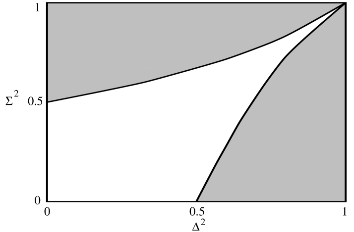
FIG. 12.: Schema showing the regions of antirigidity (shaded) and rigidity for the helical breather at $\beta=1$. Here $\Delta^{2}=1-q^{2}$ and $\Sigma=\sin(\tau_{0})$.

TABLE I.: The numerical coefficients appearing in the action to fourth order for some values of the Bogomol’nyi parameter $\beta$.

$\beta$	$\mu/\pi\eta^{2}$	$\alpha_{1}/\pi\eta^{2}$	$\alpha_{2}/\pi$	$\alpha_{3}/\pi$
$0.1$	$3.272$	$6.025$	$77.761$	$-104.985$
$0.2$	$2.813$	$3.347$	$23.565$	$-32.835$
$0.5$	$2.314$	$1.634$	$4.308$	$-6.767$
$1.0\leavevmode\leavevmode\hbox{${}^{\rm a}$}$	$2.000$	$0.999$	$1.069$	$-2.138$
$2.0$	$1.736$	$0.642$	$0.174$	$-0.722$
$10.0$	$1.278$	$0.272$	$-0.097$	$-0.094$
$50.0$	$0.977$	$0.141$	$-0.065$	$-0.030$
$100.0$	$0.880$	$0.111$	$-0.052$	$-0.023$

REFERENCES

[1] E-mail: manderso@scorpion.cowan.edu.au
[2] E-mail: Filipe.Bonjour@durham.ac.uk
[3] E-mail: R.A.W.Gregory@durham.ac.uk
[4] E-mail: john@amtp.cam.ac.uk
[5] A. Vilenkin and E. P. S. Shellard, Cosmic Strings and
Other Topological Defects (Cambridge University Press,
Cambridge, 1994).
[6] T. Vachaspati and A. Achúcarro, Phys. Rev. D 44,
3067 (1991); M. Hindmarsh, Phys. Rev. Lett. 68,
1263 (1991).
[7] T. Vachaspati, Phys. Rev. Lett. 68, 1977 (1992);
Phys. Rev. Lett. 69, 216(E) (1992);
N. Manton, Phys. Rev. D 28, 2019 (1983).
[8] N. Turok, Phys. Rev. Lett. 63, 2625 (1989).
[9] R. Brandenberger, Modern Cosmology and Structure
Formation [astro-ph/9411049];
M. Hindmarsh and T. W. B. Kibble, Rep. Prog. Phys. 58,
477 (1995) [hep-ph/9411342].
[10] E. P. S. Shellard, Nucl. Phys. B 283, 624 (1987);
K. J. M. Moriarty, E. Myers and C. Rebbi, Phys. Lett.
207, 411 (1988).
[11] A. Vilenkin, Phys. Rev. D 23, 852 (1981);
J. R. Gott III, Astrophys. J. 288, 422 (1985);
W. Hiscock, Phys. Rev. D 31, 3288 (1985);
B. Linet, Gen. Relativ. Grav. 17, 1109 (1985);
D. Garfinkle, Phys. Rev. D 32, 1323 (1985);
R. Gregory, Phys. Rev. Lett. 59, 740 (1987).
[12] T. Vachaspati and A. Vilenkin, Phys. Rev. Lett. 67,
1057 (1991); D. N. Vollick, Phys. Rev. D 45, 1884
(1992).
[13] K.-i. Maeda and N. Turok, Phys. Lett. 202B, 376 (1988);
R. Gregory, Phys. Lett. 206B, 199 (1988).
[14] D. Garfinkle and R. Gregory, Phys. Rev. D 41, 1889
(1990);
R. Gregory, D. Haws and D. Garfinkle, Phys. Rev. D 42,
343 (1990);
R. Gregory, Phys. Rev. D 43, 520 (1991).
[15] V. Silveira and M. D. Maia, Phys. Lett. 174A, 280
(1993) [gr-qc/9303017];
P. Orland, Nucl. Phys. B 428, 221 (1994)
[hep-th/9404140];
H. Arodź, Nucl. Phys. B 450, 174 (1995)
[hep-th/9502018];
Nucl. Phys. B 450, 189 (1995) [hep-th/9503001].
[16] H. B. Nielsen and P. Olesen, Nucl. Phys. B 61, 45
(1973).
[17] D. Förster, Nucl. Phys. B 81, 84 (1974).
[18] B. Carter and R. Gregory, Phys. Rev. D 51, 5839
(1995) [hep-th/9410095].
[19] M. Anderson, Phys. Rev. D 51, 2863 (1995).
[20] T. L. Curtright, G. I. Ghandour and C. K. Zachos, Phys.
Rev. D 34, 3811 (1986);
B. Boisseau and P. S. Letelier, Phys. Rev. D 46, 1721
(1992);
H. Arodź and A. L. Larsen, Phys. Rev. D 49, 4154
(1994) [hep-th/9309089].
[21] A. Polyakov, Nucl. Phys. B 268, 406 (1986).
[22] H. Kleinert, Phys. Lett. 174B, 335 (1986).
[23] B. Carter, Class. Quantum Grav. 11, 2677 (1994).
[24] T. W. B. Kibble and N. Turok, Phys. Lett. 116B, 141
(1982).
[25] D. Garfinkle and T. Vachaspati, Phys. Rev. D 42, 1960
(1990).
[26] M. Sakellariadou, Phys. Rev. D 42, 453 (1990);
Phys. Rev. D 43, 4150(E) (1991).
[27] M. Spivak, Differential Geometry (Publish or Perish,
Berkeley, CA, 1979).
[28] B. Carter, J. Geom. Phys. 8, 53 (1992);
[hep-th/9705172].
[29] Numerical Algorithms Group, NAG Fortran Library Mark 16
(Oxford, 1993).
[30] W. H. Press, S. A. Teukolski, W. T. Vetterling and
B. P. Flannery, Numerical Recipes in C: the Art of
Scientific Computing (Cambridge University Press,
Cambridge, 1992).