TTP96–18
May 1996

Theory of Top Quark Production and Decay^†
J.H. Kühn

Institut für Theoretische Teilchenphysik, Universität Karlsruhe

D-76128 Karlsruhe, Germany

email: johann.kuehn@physik.uni-karlsruhe.de

Abstract

Direct and indirect information on the top quark mass and its decay modes is reviewed. The theory of top production in hadron- and electron-positron-colliders is presented.

^†Lectures presented at XXIII SLAC Summer Institute on Particle Physics, “The Top Quark and the Electroweak Interaction,” July 10–21, 1995, SLAC, Stanford, CA.
Supported by BMBF 057KA92P and Volkswagen-Stiftung grant I/70452.

Introduction

An extensive search for top quarks has been performed at electron-positron and hadron colliders for more than a decade. First evidence for top quark production in proton-antiproton collisions has been announced by the CDF collaboration in the spring of 1994. After collecting more luminosity subsequently both the CDF and the D0 experiments presented the definite analysis [1] which demonstrated not only the existence of the anticipated quark but at the same time also provided a kinematic determination of the top quark mass around 180 GeV and a production cross section consistent with the QCD predictions. The mass value is in perfect agreement with the indirect mass determinations based on precision measurements [2-7] of the electroweak parameters in $e^{+}e^{-}$annihilation and in lepton-nucleon scattering. Exploiting the quadratic top mass dependence of radiative corrections an indirect mass measurement of 180 GeV with a present uncertainty of roughly $20$ GeV has been achieved.

The top quark completes the fermionic spectrum of the Standard Model. All its properties are uniquely fixed after the mass has been determined. However, as a consequence of its large mass and decay rate it will behave markedly different compared to the remaining five lighter quarks.

It is not just the obvious aim for completion which raises the interest in the top quark. With its mass comparable to the scale of the electroweak symmetry breaking it is plausible that top quark studies could provide an important clue for the understanding of fermion mass generation and the pattern of Yukawa couplings. In fact, it has been suggested that a top quark condensate could even be responsible for the mechanism of spontaneous symmetry breaking [8].

These lectures will be mainly concerned with top quark phenomenology within the framework of the Standard Model (SM). The precise understanding of its production and decay constitutes the basis of any search for deviations or physics beyond the SM.

The properties of the top quark will be covered in chapter 1. Direct and indirect determinations of its decay rates, decay distributions including QCD and electroweak corrections and decay modes predicted in supersymmetric extensions will be discussed. Top quark production at hadron colliders will be the subject of chapter 2. The production cross section and momentum distributions are important ingredients in any of the present analysis. An alternative reaction, namely top quark production through $W$-$b$-fusion allows to determine the $W$-$b$-$\bar{t}$ coupling and thus indirectly the top quark decay rate.

Perspectives for top studies at a future $e^{+}e^{-}$collider will be presented in chapter 3. An accurate determination of the top quark mass and its width to better than 1 GeV with a relative accuracy of about 10% seems feasible, and the electroweak couplings of the top quark could be precisely measured with the help of polarized beams. Of particular interest is the interplay between the large top quark decay rate and the binding through the QCD potential which will be also covered in chapter 3.

Chapter 1 The Profile of the Top Quark

Hadron collider experiments at the TEVATRON have firmly established the existence of the top quark and already provide a fairly accurate determination of its mass. The couplings of the top quark to the gauge bosons are uniquely fixed by the SM. Thus all its properties — its production cross section and its decay rate and distributions — can be predicted unambiguously.

The study of real top quarks at high energy colliders, in particular the observation of a peak in the invariant mass of its decay products, is certainly the most impressive proof of existence. Nevertheless, the indirect evidence for a top quark and the determination of its mass is not only of historical interest. The arguments which anticipated the existence of the top quark and its mass around 180 GeV illustrate the rigid structure of the SM, its selfconsistency and beauty. They will be presented in section 1.1.

These theoretical arguments have inspired the experimental searches. The upper limit on the top mass around 200 GeV deduced already relatively early from electroweak precision studies has provided encouragement that energies of present colliders were suited to complete this enterprise. The agreement between the most recent indirect mass determinations both through radiative corrections and through direct observation strengthens the present belief into the quantum field aspect of the theory. It furthermore justifies the corresponding line of reasoning concerning the search for the last remaining ingredient of the SM, the Higgs boson. Section 1.1 of this first chapter will, with this motivation in mind, be devoted to a discussion of the indirect information on the top quark, its existence and its mass. Top decays, including aspects of radiative corrections, polarisation effects and decays induced by physics beyond the SM will be covered in section 1.2.

1.1 Indirect information

1.1.1 Indirect evidence for the top quark

Several experimental results already prior to its discovery did provide strong evidence that the fermion spectrum of the Standard Model

$${\left[\nu_{e}\atop e^{-}\right]_{L}}\quad{\atop e^{-}_{R}}\qquad{\left[\nu_{\mu}\atop\mu^{-}\right]_{L}}\quad{\atop\mu^{-}_{R}}\qquad{\left[\nu_{\tau}\atop\tau^{-}\right]_{L}}\quad{\atop\tau^{-}_{R}}$$

$$\!{\left[{\;u\;}\atop d\right]_{L}}\quad{u_{R}\atop d_{R}}\qquad{\left[{\,\,c\,\,}\atop s\right]_{L}}\quad{c_{R}\atop s_{R}}\qquad\,{\left[{\,\,t\,\,}\atop b\right]_{L}}\quad{t_{R}\atop b_{R}}$$

does include the top quark, imprinting the same multiplet structure on the third family as the first two families. The evidence is based on theoretical selfconsistency (absence of anomalies), the absence of flavour changing neutral currents (FCNC) and measurements of the weak isospin of the $b$ quark which has been proved to be non-zero, $I_{3}=-1/2$, thus demanding an $I_{3}=+1/2$ partner in this isospin multiplet.

Absence of triangle anomalies

A compelling argument for the existence of top quarks follows from a theoretical consistency requirement. The renormalizability of the Standard Model demands the absence of triangle anomalies. Triangular fermion loops built-up by an axialvector charge $I_{3A}=-I_{3L}$ combined with two electric vector charges $Q$ would spoil the renormalizability of the gauge theory. Since the anomalies do not depend on the masses of the fermions circulating in the loops, it is sufficient to demand that the sum

$$\sim\sum_{L}I_{3A}Q^{2}=-\sum_{L}I_{3}\left[I_{3}+\frac{1}{2}Y\right]^{2}$$

$$\sim\sum_{L}Y\sim\sum_{L}Q$$

of all contributions be zero. Such a requirement can be translated into a condition on the electric charges of all the left-handed fermions

$$\sum_{L}Q=0.$$ (1.1)

This condition is met in a complete standard family in which the electric charges of the lepton plus those of all color components of the up and down quarks add up to zero,

$$\sum_{L}Q=-1+3\times\left[\left(+\frac{2}{3}\right)+\left(-\frac{1}{3}\right)\right]=0.$$

If the top quark were absent from the third family, the condition would be violated and the Standard Model would be theoretically inconsistent.

Absence of FCNC decays

Mixing between quarks which belong to different isospin multiplets

$${\left[c\atop s^{{}^{\prime}}\right]_{L}}\quad{\atop b^{{}^{\prime}}_{L}}\hskip 56.9055pt{\!s^{{}^{\prime}}_{L}=\>s_{L}\cos\vartheta^{{}^{\prime}}+b_{L}\sin\vartheta^{{}^{\prime}}\atop\>b_{L}^{{}^{\prime}}=-s_{L}\sin\vartheta^{{}^{\prime}}+b_{L}\cos\vartheta^{{}^{\prime}}}$$

generates non-diagonal neutral current couplings, i.e. the breaking of the GIM mechanism

$$<I_{3}> = +\frac{1}{2}\left(\bar{c}_{L},c_{L}\right)-\frac{1}{2}\left(\bar{s}^{{}^{\prime}}_{L},s^{{}^{\prime}}_{L}\right)$$

$$= {1\over 2}\left(\bar{c}_{L},c_{L}\right)--{1\over 2}\left(\bar{s}_{L},s_{L}\right)\cos^{2}\vartheta^{\prime}-{1\over 2}\left(\bar{b}_{L},b_{L}\right)\sin^{2}\vartheta^{\prime}$$

$$-\frac{1}{2}\sin\vartheta^{{}^{\prime}}\cos\vartheta^{{}^{\prime}}\left(\left(\bar{s}_{L},b_{L}\right)+\left(\bar{b}_{L},s_{L}\right)\right).$$

The non-diagonal current induces flavor-changing neutral lepton pair decays $b\mbox{$\rightarrow$ }s+l^{+}l^{-}$ which have been estimated to be a substantial fraction of all semileptonic $B$ meson decays. The relative strenth of neutral versus charged current induced rate is essentially given by

$${\Gamma_{\rm NC}\over\Gamma_{\rm CC}}\sim{1\over 2}\left({M_{W}^{2}\over M_{Z}^{2}}\right)^{2}{(v_{b}^{2}+a_{b}^{2})(v_{e}^{2}+a_{e}^{2})\over(1+1)(1+1)}\sim 0.06.$$ (1.2)

Taking the proper momentum dependence of the matrix element and the phase space into account one finds [9]

$$\frac{\mbox{BR}\left(B\mbox{$\rightarrow$ }l^{+}l^{-}X\right)}{\mbox{BR}\left(B\mbox{$\rightarrow$ }l^{+}\nu_{l}X\right)}\geq 0.12.$$ (1.3)

This ratio is four orders of magnitude larger than a bound set by the UA1 Collaboration [10, 11]

$$\frac{\mbox{BR}\left(B\mbox{$\rightarrow$ }\mu^{+}\mu^{-}X\right)}{\mbox{BR}\left(B\mbox{$\rightarrow$ }\mu\nu_{\mu}X\right)}<\frac{5.0\times 10^{-5}}{0.103\pm 0.005}.$$ (1.4)

so that the working hypothesis of an isosinglet $b$ quark is clearly ruled out experimentally also by this method.

Partial width $\Gamma(Z\mbox{$\rightarrow$ }\mbox{$b\overline{b}$})$ and forward-backward asymmetry of $b$ quarks

The $Z$ boson couples to quarks through vector and axial–vector charges with the well–known strength

$$\psfig{width=99.58464pt,bbllx=210pt,bblly=410pt,bburx=630pt,bbury=550pt}=\sqrt{\frac{G_{F}m_{Z}^{2}}{2\sqrt{2}}}\gamma_{\mu}\left[v_{q}-a_{q}\gamma_{5}\right].$$

Depending on the isospin assignment of righthanded and lefthanded quark fields these charges are defined as

$$v_{q} = 2(I_{q}^{3L}+I_{q}^{3R})-4e_{q}\sin^{2}\vartheta_{W}$$ (1.5)

$$a_{q} = 2(I_{q}^{3L}-I_{q}^{3R})$$ (1.6)

For the present application the Born approximation in the massless limit provides an adequate representation of the partial $Z$ decay rate

$$\Gamma_{B}(Z\rightarrow b\overline{b})\approx\frac{G_{F}m_{Z}^{3}}{8\sqrt{2}\pi}\beta\left(v_{b}^{2}+a_{b}^{2}\right).$$ (1.7)

In the Standard Model $2I_{q}^{3R}=0$ and $2I_{q}^{3L}=\pm 1$ for up/down quarks respectively.

The ratio between the predictions in the context of a topless model and the SM amounts to

$${\Gamma^{\rm topless}\over\Gamma^{\rm SM}}={(4Q_{b}\sin^{2}\theta_{W})^{2}\over(1+4Q_{b}\sin^{2}\theta_{W})^{2}+1}\approx 1/13$$ (1.8)

whereas theory and LEP experiments are well consistent

$${\Gamma(Z\to b\bar{b})\over\Gamma(Z\to{\rm had})}=\left\{\begin{array}[]{lll}0.2155\pm 0.0004&{\rm theory}&\cite[cite]{[\@@bibref{}{HollikBrus}{}{}]}\\ 0.2219\pm 0.0017&{\rm experiment}&\cite[cite]{[\@@bibref{}{HollikBrus}{}{}]}\end{array}\right.$$ (1.11)

ruling out the $I=0$ assignement for the $b$-quark. The forward-backward asymmetry at the $Z$ resonance

$$A^{\rm FB}={3\over 4}A_{e}A_{b}$$ (1.12)

with

$$A_{f}\equiv{2v_{f}a_{f}\over v_{f}^{2}+a_{f}^{2}}$$ (1.13)

is sensitive toward the relative size of vector and axial $b$ quark couplings. Up to a sign, the first of these factors, $A_{e}\approx 0.15$, can be interpreted as the degree of longitudinal $Z$ polarisation, $P_{Z}=-A_{e}$, which is induced by the electron coupling even for unpolarized beams. For longitudinally polarized beams it can be replaced by unity. The second factor represents essentially the analyzing power of $b$ quarks. With a predicted value of 0.93 it is close to its maximum in the SM. In fact, this high analysing power is the reason for the large sensitivity of $A^{FB}$ toward $\sin^{2}\theta_{W}$ [12]. For a fictitious topless model $A_{b}$ is zero. The most recent experimental results from LEP and SLC are displayed in Fig. 1.1.

Figure 1.1: Experimental results for the asymmetry parameter $A_{b}$ [13].

A remaining sign ambiguity is finally resolved by the interference between NC and electromagnetic amplitude. It leads to a forward backward asymmetry at low energies

$$A_{\rm FB}=-{3G_{F}s\over 16\sqrt{2}\pi\alpha}{a_{e}a_{b}\over Q_{e}Q_{b}}$$ (1.14)

which has been studied in particular at PEP, PETRA, and most recently with highest precision at Tristan at a cm energy of 58 GeV [14]. Using the data available shortly after the turnon of LEP and combining $\Gamma_{b\bar{b}}$, $A_{b}$, and $A_{\rm FB}$

$$\hskip 0.0pt minus 1.0fil\{I_{3}^{L}(b)\}_{exp}=-0.490^{+0.015}_{-0.012}\hfill \rightarrow I_{3}^{L}(b)=-1/2$$

$$\{I_{3}^{R}(b)\}_{exp}=-0.028{\pm 0.056} \rightarrow I_{3}^{R}(b)=0$$

has been obtained already some time ago [15]. As shown in Fig. 1.2 all measurements are nicely consistent with the predictions of the SM. The isospin assignment of the Standard Model is thus well confirmed.

Figure 1.2: The weak isospins $I_{3}^{L}(b)$ and $I_{3}^{R}(b)$ of the left– and right–handed $b$ quark components, extracted from the data on $\Gamma(Z\mbox{$\rightarrow$ }b\overline{b})$ and $A_{FB}(b)$ at LEP, and PETRA/PEP and TRISTAN, Ref.[15].

1.1.2 Mass limits and indirect mass determinations

Theoretical constraints

Present theoretical analyses of the Standard Model are based almost exclusively on perturbation theory. If this method is assumed to apply also to the top-quark sector, in particular when linked to the Higgs sector, the top mass must be bounded as the strength of the Yukawa-Higgs-top coupling is determined by this parameter. The following consistency conditions must be met:

Perturbative Yukawa coupling $g_{Y}\left(ttH\right)$

Defining the Yukawa coupling in the Standard Model  through

$${\cal L}_{Y}=g_{Y}\left({v+H\over\sqrt{2}}\right)\left(\bar{t}_{L}t_{R}+\mbox{h.c.}\right)$$ (1.15)

the coupling constant $g_{Y}$ is related to the top mass by

$$g_{Y}\left(ttH\right)=m_{t}\sqrt{2\sqrt{2}G_{F}}.$$ (1.16)

Demanding the effective expansion parameter $g^{2}_{Y}/4\pi$ to be smaller than 1, the top mass is bounded to

$$m_{t}<\sqrt{\frac{\sqrt{2}\pi}{G_{F}}}\approx 620\mbox{GeV}.$$ (1.17)

For a top mass of 180 GeV the coupling $g^{2}_{Y}/4\pi\approx 0.085$ is comfortably small so that perturbation theory can safely be applied in this region.

Unitarity bound
At asymptotic energies the amplitude of the zeroth partial wave for elastic $t\overline{t}$ scattering in the color singlet same-helicity channel [16]

$$a_{0}\left(\mbox{$t\overline{t}$}\mbox{$\rightarrow$ }\mbox{$t\overline{t}$}\right) = -\frac{3g^{2}_{Y}}{8\pi}$$

$$= -\frac{3G_{F}m^{2}_{t}}{4\sqrt{2}\pi}$$

grows quadratically with the top mass. Unitarity however demands this real amplitude to be bounded by $\left|\mbox{Re}\,a_{0}\right|\leq 1/2$. This condition translates to

$$m_{t}<\sqrt{\frac{2\sqrt{2}\pi}{3G_{F}}}\approx 500\,\mbox{GeV}.$$ (1.19)

The bound improves by taking into account the running of the Yukawa coupling [17]. These arguments are equally applicable for any additional species of chiral fermions with mass induced via spontaneous symmetry breaking.

Stability of the Higgs system: top-Higgs bound
The quartic coupling $\lambda$ in the effective Higgs potential

$$V=\mu^{2}\left|\phi\right|^{2}+\frac{\lambda}{2}\left|\phi\right|^{4}$$

depends on the scale at which the system is interacting. The running of $\lambda$ is induced by higher-order loops built-up by the Higgs particles themselves, the vector bosons and the fermions in the Standard Model [17, 18]. For moderate values of the top mass, $m_{t}\leq 77$ GeV, these radiative corrections would have generated a lower bound on the Higgs mass of 7 GeV. With the present experimental lower limit $m_{H}>65$ GeV and the top quark mass determined around 180 GeV this bound is of no practical relevance any more. At high energies the radiative corrections make $\lambda$ rise up to the Landau pole at the cut-off parameter $\Lambda$ beyond which the Standard Model in the present formulation cannot be continued [“triviality bound”, as this bound could formally be misinterpreted as requiring the low energy coupling to vanish]. If for a fixed Higgs mass the top mass is increased, the top loop radiative corrections lead to negative values of the quartic coupling $\lambda$

$$\frac{\partial\lambda}{\partial\log s}=\frac{3}{8\pi^{2}}\left[\lambda^{2}-4g^{4}_{Y}+\mbox{gauge couplings}\right]$$ (1.20)

Since the potential is unbounded from below in this case, the Higgs system becomes instable. Thus the stability requirement defines an upper value of the top mass $m_{t}$ for a given Higgs mass $m_{H}$ and a cut-off scale $\Lambda$. The result of such an analysis is presented in Fig.1.3. Depending on the cut-off scale $\Lambda$ where new physics may set in,

Figure 1.3: Bounds on the Higgs and top masses following from triviality of the Higgs’s quartic self-coupling and the stability of the Higgs system; from [18].

the top mass is bounded to $m_{t}\leq 200$ GeV if $\Lambda$ exceeds the Planck scale but it rises up to 400 to 500 GeV if the cut-off is reached at a level of 1 TeV and below. The estimates are similar to the unitarity analysis in the preceeding subsection. Lattice simulations of the Yukawa model have arrived at qualitatively similar results (see e.g. [19]).

These theoretical analyses have shown that for the top mass around 180 GeV the Standard Model may be valid up to a cut-off at the Planck scale. [The hierarchy problem, that is not touched in the present discussion, may enforce nevertheless new additional physical phenomena already in the TeV range.]

In the context of the SM the top Yukawa coupling is simply present as a free parameter. In the minimal supersymmetric model, however, the picture is changed completely. A large Yukawa coupling may play the role of a driving term for the spontaneous breaking of $SU(2)\times U(1)$, as discussed in [20] and in fact the large mass of the top quark had been predicted on the basis of these arguments prior to its experimental discovery.

Mass estimates from radiative corrections

First indications of a high top quark mass were derived from the rapid $(B-\overline{B})$ oscillations observed by ARGUS [21]. However, due to the uncertainties of the $CKM$ matrix element $V_{td}$ and of the $(b\bar{d})$ wave function, not more than qualitative conclusions can be drawn from such an analysis as the oscillation frequency $\Delta m\sim\left|V_{td}\right|^{2}f^{2}_{B}m^{2}_{t}$ depends on three [unknown] parameters.

The analysis of the radiative corrections to high precision electroweak observables is much more advanced [2-7]. Since Higgs mass effects are weak as a result of the screening theorem [22], the top mass is the dominant unknown in the framework of the Standard Model. Combining the high precision measurements of the $Z$ mass with $\sin^{2}\theta_{W}$ from the $Z$ decay rate, from the forward-backward asymmetry and from LR polarization measurements, the top quark mass has been determined up to a residual uncertainty of less than 10 GeV plus an additional uncertainty of about 20 GeV induced through the variation of $m_{H}$

$$m_{t}=178\pm 8^{+17}_{-20}\;{\rm GeV}.$$ (1.21)

The close agreement between direct and indirect top mass determination can be considered a triumph of the Standard Model. Its predictions are not only valid in Born approximation, as expected for any effective theory, also quantum corrections play an important role, and are indirectly confirmed. Encouraged by this success and in view of the improved accuracy of theory and experiment it is conceivable that the same strategy can lead to a rough determination of the Higgs mass, or, at least, to a phenomenologically relevant upper limit.

1.1.3 The quadratic top mass dependence of $\delta\rho$

The quadratic top mass dependence of $\delta\rho$ is a cornerstone of the present precision measurements [23]. In view of its importance and the pedagogical character of these lectures it is perhaps worthwhile to present a fairly pedestrian derivation of this result.

Let us first consider the definition of the weak mixing angle in Born approximation. It can be fixed through the relative strength of charged vs. neutral current couplings:

$$= {g\over 2\sqrt{2}}\gamma_{\mu}(1-\gamma_{5})$$ (1.22)

$$= {g\over 4\cos\bar{\theta}_{W}}\left[\left(2I_{3}^{f}-4Q_{f}\sin^{2}\bar{\theta}_{W}\right)\gamma_{\mu}+2I_{3}^{f}\gamma_{\mu}\gamma_{5}\right]$$ (1.23)

with the SU(2) coupling related to the electromagnetic coupling through $g=e/\sin\bar{\theta}_{W}$. Alternatively $\sin^{2}\theta_{W}$ is defined through the mass ratio

$$M_{W}^{2}/M_{Z}^{2}=1-\sin^{2}\theta_{W}$$ (1.24)

These two definitions coincide in Born approximation

$$\theta_{W}=\left.\bar{\theta}_{W}\right|_{\rm Born}$$ (1.25)

However, the self energy diagrams depicted in Fig. 1.4 lead to marked differences between the two options, in particular if $m_{t}\gg M_{W,Z}\gg m_{b}$.

Figure 1.4: Self energy diagrams which induce the mass splitting between $W^{\pm}$ and $W^{0}$ and a $\rho$ parameter different from one.

This difference can be traced to a difference in the mass shift for the $W$ and the $Z$ boson. For a simplified discussion consider, in a first step, $\sin^{2}\theta_{W}=0$ and hence the $SU(2)$ part of the theory only. The neutral boson will be denoted by $W^{0}$. In the lowest order this implies

$$M_{-}=M_{0}\equiv M$$ (1.26)

and the couplings simplify to

$$= {g\over 2\sqrt{2}}\gamma_{\mu}(1-\gamma_{5})$$ (1.27)

$$= {g\over 4}2I_{3}^{f}\gamma_{\mu}(1-\gamma_{5})$$ (1.28)

In order $g^{2}$ the propagators of charged and neutral bosons are modified by the self energies

$$W^{+}:\qquad\qquad{1\over M^{2}-s} \Rightarrow {1\over M^{2}-s-\Pi_{+}(s)}$$

$$W^{0}:\qquad\qquad{1\over M^{2}-s} \Rightarrow {1\over M^{2}-s-\Pi_{0}(s)}$$ (1.29)

The mass shifts individually are given by

$$\delta M_{+,0}^{2}=M_{+,0}^{2}-M^{2}=-Re\,\Pi_{+,0}(M^{2}).$$ (1.30)

They are most easily calculated through dispersion relations from their respective imaginary parts. These can be interpreted as the “decay rate” of a fictitious virtual boson of mass $\kappa$:

$$\kappa\Gamma(W_{+}^{*}\to t+\bar{b})=Im\,\Pi_{+}(\kappa^{2})$$

$$\delta M^{2}_{+}={1\over\pi}\int{d\kappa^{2}\over\kappa^{2}-M^{2}}Im\,\Pi_{+}(\kappa^{2}).$$ (1.31)

The decay rates of the virtual bosons are easily calculated ($m\equiv m_{top}$)

$$\kappa\Gamma(W_{+}^{*}\to t\bar{b})={3\over 12\pi}\left(g\over 2\sqrt{2}\right)^{2}\kappa^{2}2\left(1-{m^{2}\over 2\kappa^{2}}-{m^{4}\over 2\kappa^{4}}\right)\left(1-{m^{2}\over\kappa^{2}}\right)\Theta(\kappa^{2}-m^{2}).$$ (1.32)

The factor 3 originates from color, the factor 2 from the identical vector and axial contributions, the squared matrix element and the phase space are responsible for the second and third factors in brackets respectively.

Similarly one finds

$$\kappa\Gamma(W_{0}^{*}\to b\bar{b})+\kappa\Gamma(W_{0}^{*}\to t\bar{t})=$$

$${3\over 12\pi}\left(g\over 4\right)^{2}\kappa^{2}\left\{2\Theta(\kappa^{2})+2\left(1-{m^{2}\over\kappa^{2}}\right)\left(1-{4m^{2}\over\kappa^{2}}\right)^{1/2}\Theta(\kappa^{2}-4m^{2})\right\}$$

$$\delta M^{2}_{0}={1\over\pi}\int{d\kappa^{2}\over\kappa^{2}-M^{2}}Im\,\Pi_{0}(\kappa^{2}).$$ (1.33)

With the large $\kappa^{2}$ behaviour of ${\rm Im}\,\Pi$ given by ${\rm Im}\,\Pi\sim\kappa^{2}$ the dispersive integral eq. (1.31) is evidently quadratically divergent. In the limit of large $\kappa$ the leading ($\sim\kappa^{2}$) and next-to-leading ($\to$ const) terms of eqs. (1.32) and (1.33) coincide. The leading and next to leading divergences can therefore be absorbed in a $SU(2)$ invariant mass renormalization. The relative mass shift, however, the only quantity accessible to experiment, remains finite and is given by

$$\delta M^{2} = \delta M^{2}_{+}-\delta M^{2}_{0}$$ (1.37)

$$= {3\over 12\pi}{g^{2}\over 8}{1\over\pi}\int_{0}^{\infty}{d\kappa^{2}\over\kappa^{2}-M^{2}}\kappa^{2}$$

$$\times\left\{\begin{array}[]{ll}-2\left(1-{m^{2}\over\kappa^{2}}\right)\left(1-{m^{2}\over 2\kappa^{2}}-{m^{4}\over 2\kappa^{4}}\right)&\times\Theta(\kappa^{2}-m^{2})\\ +1&\times\Theta(\kappa^{2})\\ \left(1-{m^{2}\over\kappa^{2}}\right)\left(1-{4m^{2}\over\kappa^{2}}\right)^{1/2}&\times\Theta(\kappa^{2}-4m^{2})\end{array}\right.$$

We are only interested in the leading top mass dependence: $m^{2}\gg M^{2}$. The leading term is obtained by simply setting $M^{2}\to 0$ in the integrand. Introducing a cutoff $\Lambda^{2}\gg m^{2}$ the leading contributions to the three integrals are given by

$$\left\{\rule{-2.84526pt}{14.22636pt}\right. -2\Lambda^{2}+3m^{2}\ln{\Lambda^{2}\over m^{2}}+{3\over 2}m^{2}+\ldots$$ (1.38)

$$+\Lambda^{2}$$

$$+\Lambda^{2}-3m^{2}\ln{\Lambda^{2}\over m^{2}}\left.\rule{-2.84526pt}{14.22636pt}\right\}$$

and hence

$$\delta M^{2}={3\over 12\pi^{2}}{g^{2}\over 8}{3\over 2}m^{2}$$ (1.39)

Up to the proportionality constant this result could have been guessed on dimensional grounds from the very beginning.

It has become customary to express the $SU(2)$ coupling in terms of $G_{F}$ and the $W$ mass

$${g^{2}\over 8}={G_{F}\over\sqrt{2}}M_{W}^{2}$$ (1.40)

such that

$${\delta M^{2}\over M^{2}}={3\over 16\pi^{2}}\sqrt{2}G_{F}m^{2}.$$ (1.41)

The ratio of neutral versus charged current induced amplitude at small momentum transfers is thus corrected by a factor

$${M_{+}^{2}\over M_{0}^{2}}\equiv 1+\delta\rho=\left(1+{\delta M^{2}\over M^{2}}\right)$$ (1.42)

with $\delta\rho$ given in eq. (1.41).

To discuss the phenomenological implications of this result it is now necessary to reintroduce the weak mixing between the neutral $SU(2)$ and $U(1)$ gauge bosons. The gauge boson masses are induced by the squared covariant derivative acting on the Higgs field

$$D_{\mu}\phi\to-i\left(g\vec{W}_{\mu}{\vec{\tau}\over 2}+g^{\prime}BY\right)\left(\begin{array}[]{c}0\\ v/\sqrt{2}\end{array}\right)$$ (1.45)

giving rise to the following mass terms in the Lagrangian

$${\cal L}_{M} = {v^{2}\over 8}(g^{2}+g^{\prime 2})\left({g\over\sqrt{g^{2}+g^{\prime 2}}}W_{3}-{g^{\prime}\over\sqrt{g^{2}+g^{\prime 2}}}B\right)^{2}$$ (1.46)

$$+{v^{2}\over 8}g^{2}(W_{1}^{2}+W_{2}^{2})(1+\delta\rho)$$

The last term has been added to represent a contribution from a non vanishing $\delta\rho$, induced e.g. by the large top mass. The finite mass shift has been without loss of generality entirely attributed to the charged $W$ boson.

The mass eigenstates are easily identified from eq. (1.46)

$$W^{\pm} = (W_{1}\mp iW_{2})/\sqrt{2}$$

$$Z = (\bar{c}W_{3}-\bar{s}B)$$

$$A = (\bar{c}B+\bar{s}W_{3})$$ (1.47)

with the weak mixing angle $\bar{\theta}_{W}$

$$\bar{c}\equiv\cos\bar{\theta}_{W}\equiv{g\over\sqrt{g^{2}+g^{\prime 2}}}$$

$$\bar{s}\equiv\sin\bar{\theta}_{W}\equiv{g^{\prime}\over\sqrt{g^{2}+g^{\prime 2}}}$$ (1.48)

defined through the couplings. This definition is, of course, very convenient for measurements at LEP, where couplings are determined most precisely. The couplings of the photon and the $Z$ boson are thus also given in terms of $\bar{s}$. The masses are read off from eq. (1.46)

$$m_{A}^{2} = 0$$

$$m_{Z}^{2} = {v^{2}\over 4}(g^{2}+g^{\prime 2})$$

$$m_{W}^{2} = {v^{2}\over 4}g^{2}(1+\delta\rho)$$ (1.49)

and

$${m_{W}^{2}\over m_{Z}^{2}}=\bar{c}^{2}(1+\delta\rho)$$ (1.50)

which constitutes the standard definition of the $\rho$ parameter. Alternatively one may define the mixing angle directly through the mass ratio

$$s^{2}\equiv\sin^{2}\theta_{W}\equiv 1-M_{W}^{2}/M_{Z}^{2}$$ (1.51)

The two definitions coincide in the Born approximation; they differ, however, for $\delta\rho\neq 0$:

$$s^{2}=1-\bar{c}^{2}(1+\delta\rho)=\bar{s}^{2}-\bar{c}^{2}\delta\rho$$ (1.52)

It is, of course, a matter of convention and convenience, which of the two definitions (or their variants) are adopted. The choice of input parameters and observables will affect the sensitivity towards $\delta\rho$ — and hence towards $m_{t}$. The observables which are measured with the highest precision at present and in the forseable future are the fine-structure constant $\alpha$, the muon life time which provides a value for $G_{F}$ and the $Z$ boson mass. To obtain the dependence of $\sin^{2}\theta_{W}$ on $\delta\rho$ we predict $M_{W}^{2}$ from these observables. We start from

$${g^{2}\over 8}{1\over M_{W}^{2}}={G_{F}\over\sqrt{2}}$$ (1.53)

and express $g^{2}$ through $G_{F}$ and $M_{Z}^{2}$

$$g^{2}=4\sqrt{2}G_{F}M_{Z}^{2}c^{2}$$ (1.54)

Alternatively $g$ can be related to the fine structure constant

$$g^{2}=e^{2}/\bar{s}^{2}$$ (1.55)

Note the appearance of $c^{2}$ in eq. (1.51) and of $\bar{s}^{2}$ in eq. (1.48).

One thus arrives at

$$e^{2}=4\sqrt{2}G_{F}^{2}M_{Z}^{2}c^{2}(s^{2}+c^{2}\delta\rho)$$ (1.56)

or, equivalently, at

$${4\pi\alpha\over 4\sqrt{2}G_{F}M_{Z}^{2}}{1\over 1+\cot^{2}\theta_{W}\delta\rho}=s^{2}c^{2}.$$ (1.57)

Solving for $\sin^{2}\theta_{W}$ (defined through the mass ratio) one obtains on one hand

$$\sin^{2}\theta_{W}\approx{1\over 2}\left[1-\sqrt{1-{4\pi\alpha\over\sqrt{2}G_{F}M_{Z}^{2}}}\;\right]-{c^{4}\over c^{2}-s^{2}}\delta\rho$$ (1.58)

where the Born values for $c^{2}$ and $s^{2}$ can be taken in the correction term. The definition of $\sin^{2}\bar{\theta}_{W}$ through the relative strength of $SU(2)$ and $U(1)$ couplings leads on the other hand to

$$\sin^{2}\bar{\theta}_{W}\approx{1\over 2}\left[1-\sqrt{1-{4\pi\alpha\over\sqrt{2}G_{F}M_{Z}^{2}}}\;\right]-{s^{2}c^{2}\over c^{2}-s^{2}}\delta\rho$$ (1.59)

For the actual evaluation the running coupling $\alpha(M_{Z})^{-1}\approx 129$ must be employed [4]. Eq. (1.58) and eq. (1.59) exhibit rather different sensitivity towards a variation of $\delta\rho$ and hence of $m_{t}$, with a ratio between the two coefficients of $c^{2}/s^{2}\approx 3.3$. For a precise comparison between theory and experiment subleading one-loop corrections must be included, and subtle differences between variants of $\bar{\theta}_{W}$ must be taken into consideration, with $\theta_{\overline{\rm MS}}$ and $\theta_{\rm eff}^{\rm lept}$ as most frequently used options [2].

With increasing experimental accuracy numerous improvements must be and have been incorporated into the theoretical predictions.

• The full one loop corrections including all subleading terms are know since long and are certainly indispensible (see [4, 2, 24, 25] and references therein).

• Two loop purely weak corrections increase proportional $(G_{F}m_{t}^{2}/16\pi^{2})^{2}$. A detailed discussion can be found in [7].

• QCD corrections are available at the two- and even three-loop level [5, 24, 25].

With $\alpha$, $G_{F}$, and $M_{Z}$ fixed one may determine $m_{t}$ either from $M_{W}$ or alternatively from $\sin^{2}\bar{\theta}_{W}$ (corresponding to a measurement of the left right asymmetry with polarised beams, the $\tau$ polarisation or forward backward asymmetries of unpolarised beams). These measurements are in beautiful agreement with the determination of $m_{t}$ in production experiments at the TEVATRON (Fig. 1.5).

Figure 1.5:

1.2 Top Decays

Various aspects of top decays have been scrutinized in the literature. The large top decay rate predicted in the SM governs top quark physics. Radiative correctons from QCD and electroweak interactions have been calculated for the decay rate and for differential distributions of the decay products. Non-standard top decays are predicted in SUSY extensions of the SM, with $t\to Hb$ and $t\to\tilde{t}\tilde{\gamma}$ as most promising and characteristic signatures. Born predictions and radiative corrections (at least in part) have been worked out also for these decay modes. Beyond that a number of even more exotic decay modes, in particular FCNC decays, have been suggested.

1.2.1 Qualitative aspects – Born approximation

The decay of the top quark into $b+W$ is governed by the following amplitude

$${\cal M}(t\to bW)={ig\over\sqrt{2}}\bar{b}\not\varepsilon^{W}{1-\gamma_{5}\over 2}t$$ (1.60)

Adopting the high energy limit ($m_{t}^{2}>M_{W}^{2}$) for the polarisation vector $\epsilon_{L}$ of the longitudinal $W$ (corresponding to helicity $h^{W}=0$)

$$\varepsilon^{W}_{L}=\left(\begin{array}[]{c}p_{3}^{W}\\ 0\\ 0\\ p_{0}^{W}\end{array}\right){1\over M_{W}}=\left(\begin{array}[]{c}p_{0}^{W}\\ 0\\ 0\\ p_{3}^{W}\end{array}\right){1\over M_{W}}+{\cal O}(M_{W}/m_{t})$$ (1.69)

the amplitude is dominated by contribution from longitudinal $W$’s

$${\cal M}_{L} = {ig\over\sqrt{2}}\bar{b}\not\varepsilon_{L}^{W}{1-\gamma_{5}\over 2}t\approx{ig\over\sqrt{2}}{m_{t}\over M_{W}}\bar{b}{1+\gamma_{5}\over 2}t$$ (1.70)

$$= i\sqrt{2}{m_{t}\over v}\bar{b}(1+\gamma_{5})t$$

This part is thus proportional to the Yukawa coupling

$$g_{Y}=\sqrt{2}{m_{t}\over v}$$ (1.71)

with a rate growing proportional $m_{t}^{3}$. In contrast, the amplitude for the decay into transverse $W$’s, is obtained with the polarisation vectors

$$\varepsilon^{\pm}_{T}={1\over\sqrt{2}}\left(\begin{array}[]{c}0\\ 1\\ \pm i\\ 0\\ \end{array}\right)$$ (1.76)

and remains constant in the high mass limit. The rate is governed by the gauge coupling $g$ and increases only linearly with $m_{t}$. The longitudinal or transversal $W$ is produced in conjunction with a lefthanded $b$ quark. The production of $W$’s with helicity $h^{W}=+1$ is thus forbidden by angular momentum conservation (see fig. 1.6).

                 $S^{t}=+1/2$ $S_{z}^{b}=+1/2$ $h^{W}=0$ $S^{t}=-1/2$ $S_{z}^{b}=+1/2$ $h^{W}=-1$ $S^{t}=\pm 1/2$ $S_{z}^{b}=+1/2$ $h^{W}=+1$

Figure 1.6: Top decays: angular momentum conservation

In total one finds

$$(h^{W}=-1):(h^{W}=0):(h^{W}=+1)=1:{m_{t}^{2}\over 2M_{W}^{2}}:0.$$ (1.77)

The implications for the angular distributions of the decay products will be discussed below. The decay rate

$$\Gamma = {G_{F}m_{t}^{3}\over 8\sqrt{2}\pi}\left(1-{M_{W}^{2}\over m_{t}^{2}}\right)^{2}\left(1+2{M_{W}^{2}\over m_{t}^{2}}\right)$$ (1.78)

$$\approx 175\,\mbox{MeV}\left({m_{t}\over M_{W}}\right)^{3}$$

increases with the third power of the quark mass and, for a realistic top mass around 180 GeV amounts to more than 1.5 GeV, exceeding significantly all hadronic scales. Before we discuss the implications of this fact let us briefly pursue the close similarity between the coupling of the longitudinal $W$ to the $tb$ system and the decay into a charged Higgs boson in a two Higgs doublet model (THDM). The decay rate is given by (see also section 1.2.4)

$$\Gamma(t\to H^{+}b)={G_{F}m_{t}^{3}\over 8\sqrt{2}\pi}\left(1-{m_{H}^{2}\over m_{t}^{2}}\right)^{2}\left[\left({m_{b}\over m_{t}}\right)^{2}\tan^{2}\beta+\cot^{2}\beta\right]$$ (1.79)

The similarity between this rate and the rate for the decay into longitudinal $W$’s is manifest from the cubic top mass dependence. The minimal value of the term in brackets is assumed for $\tan\beta=\sqrt{m_{t}/m_{b}}$. Adopting $m_{b}(\mbox{running})\approx 3$ GeV, the minimal value of the last factor amounts to about $1/30$. On the other hand, in any plausible THDM the value of $\tan\beta$ should not exceed $m_{t}/m_{b}$. The $W$ decay mode will hence never be swamped by the Higgs channel. (This fact is of course also implied by the actual observation of the top quark at the TEVATRON.) Up to this point we have, tacitely, assumed the CKM matrix element $V_{tb}$ to be close to one. In fact, in the three generation SM one predicts (90% CL)

$$V_{tb}=0.9990\pm 0.0004 \Rightarrow BR(b)\approx 1$$

$$V_{ts}=0.044\pm 0.010 \Rightarrow BR(s)\approx 0.2\%$$

$$V_{td}=0.011\pm 0.009 \Rightarrow BR(d)\approx 0.01\%$$ (1.80)

on the basis of CKM unitarity. In a four generation model, however, sizeable mixing between third and fourth generation could arise. Methods to determine the strength of $V_{tb}$ either through single top production at a hadron collider or through a direct measurement of $\Gamma_{t}$ in $e^{+}e^{-}$ colliders will be discussed below in sects. 2.3 and 3.2.

The large top decay rate provides a cutoff for the long distance QCD dynamics. The implications can be summarised in the statement: “$t$ quarks are produced and decay like free quarks” [26]. In particular the angular distributions of their decay products follow the spin 1/2 predictions. This is in marked contrast to the situation for $b$ quarks, with $B$ mesons decaying isotropically. The arguments for this claim are either based on a comparison of energy scales, or, alternatively, on a comparison of the relevant time scales.

Let us start with the first of these two equivalent viewpoints: The mass difference between $B^{**}$ and $B$ mesons amounts to 450 MeV. In the nonrelativistic quark model the $B^{**}$ is interpreted as orbitally excited $b\bar{q}$ state. With increasing mass of the heavy quark this splitting remains approximately constant: it is essentially governed by light quark dynamics. The hyperfine splitting between $B^{*}$ and $B$, in contrast, is proportional to the color magnetic moment and hence decreases $\sim 1/m_{Q}$. Given a decay rate of about 1.5 GeV it is clear that $T$-, $T^{*}$-, and $T^{**}$- mesons merge and act coherently, rendering any distinction between individual mesons meaningless. In fact even individual toponium states cease to exist. From the perturbative QCD potential an energy difference between $1S$ and $2S$ states around 1.2–1.5 GeV is predicted. This has to be contrasted with the toponium decay rate $\Gamma_{t\bar{t}}\sim 2\Gamma_{t}\sim 3$ GeV. All resonances merge and result in an excitation curve which will be discussed in chapter 3.

A similar line of reasoning is based on the comparison between different characteristic time scales: The formation time of a hadron from a locally produced $t$ quark is governed by its size which is significantly larger than its lifetime

$$\tau_{\mbox{\small Formation}}\approx\mbox{size}\approx 1/0.5\mbox{GeV}\gg\tau_{\mbox{\small Decay}}\approx 1/\Gamma_{t}$$ (1.81)

Top quarks decay before they have time to communicate hadronically with light quarks and dilute their spin orientation. For sufficiently rapid top quark decay even $t\bar{t}$ bound states cease to exist. The classical time of revolution $T_{\rm rev}$ for a Coulombic bound state is given by $\left(\alpha_{\rm eff}={4\over 3}\alpha_{s}\right)$

$$T_{\rm rev}=\pi\alpha_{\rm eff}\sqrt{{m_{\rm red}\over 2|E|^{3}}}$$ (1.82)

With $E=-\alpha_{eff}^{2}m_{\rm red}/2$ for the ground state

$$T_{\rm rev}=\pi/|E|\gg 1/\Gamma_{t\bar{t}}$$ (1.83)

is obtained. The lifetime of the $t\bar{t}$ system is too small to allow for the proper definition of a bound state with sharp binding energy.

1.2.2 Radiative corrections to the rate

Perturbative corrections to the lowest-order result affect the total decay rate as well as differential distributions. Their inclusion is a necessary prerequisite for any analysis that attempts a precision analysis of top decays. Both QCD and electroweak corrections are well under control and will be discussed in the following.

QCD corrections

The correction to the decay rate is usually written in the form

$$\Gamma=\Gamma_{\rm Born}\left(1+\delta_{QCD}\right)=\Gamma_{\rm Born}\left(1-\frac{2}{3}\frac{\alpha_{s}}{\pi}f\right)$$ (1.84)

The correction function $f$ has been calculated in [27] for nonvanishing and vanishing $b$ mass. In the limit $m^{2}_{b}/m^{2}_{t}\to 0$ the result simplifies considerably, but remains a valid approximation (Fig.1.7):

$$f = {\cal F}_{1}/{\cal F}_{0}$$

$${\cal F}_{0} = 2(1-y)^{2}(1+2y)$$

$${\cal F}_{1} = {\cal F}_{0}\left[\pi^{2}+2Li_{2}(y)-2Li_{2}(1-y)\right]$$ (1.85)

$$+4y(1-y-2y^{2})\ln y+2(1-y)^{2}(5+4y)\ln(1-y)$$

$$-(1-y)(5+9y-6y^{2}),$$

where $y=m^{2}_{W}/m^{2}_{t}$. In the limit $m^{2}_{t}\gg m^{2}_{W}$ $f$ is well approximated by $f(y)=2/3\pi^{2}-5/2-3y+9y^{2}/2-3y^{2}\ln y\approx 4$. For $m_{t}\approx 180~{}GeV$ the QCD correction amounts to

$$\delta_{QCD}\approx-3.7\alpha_{s}/\pi$$ (1.86)

and lowers the decay rate by about 10%. This has a non-negligible impact on the height and width of a toponium resonance or its remnant.

Figure 1.7: QCD correction function $f$ for the top quark decay rate. Solid line: exact form; dashes: $m_{b}=0$, dotted: approximate form for large $m_{t}/M_{W}$.

The $\alpha_{s}^{2}$ corrections are presently unknown, and the scale $\mu$ in $\alpha_{s}(\mu^{2})$ is uncertain. Indications for a surprisingly large correction of order $\alpha_{s}^{2}$, corresponding to a rather small scale have been obtained recently. Diagrams with light fermion insertions into the gluon propagator have been calculated numerically [28] and analytically [29] in the limit $m_{t}\gg M_{W}$

$$\Gamma = \Gamma_{\rm Born}\left[1-{2\over 3}{\alpha_{\overline{\rm MS}}(m^{2}_{t})\over\pi}\left(4\zeta_{2}-{5\over 2}\right)\right.$$ (1.87)

$$+\left.\left({\alpha_{\overline{\rm MS}}\over\pi}\right)^{2}\left(-{2n_{f}\over 3}\right)\left({4\over 9}-{23\over 18}\zeta_{2}-\zeta_{3}\right)\right]$$

The BLM prescription [30] suggests that the dominant $\alpha_{s}^{2}$ coefficients can be estimated through the replacement

$$-{2n_{f}\over 3}\to\left(11-{2n_{f}\over 3}\right)$$ (1.88)

and absorbed through a change in the scale. For the problem at hand this corresponds to a scale $\mu=0.122m_{t}$ resulting in a fairly large effective value of $\alpha_{s}$ of $0.15$ instead of 0.11 for $\mu=m_{t}$.

Electroweak corrections

Electroweak corrections to the top quark decay rate can be found in [31, 32]. They involve a large number of diagrams. For asymptotically large top masses the Higgs exchange diagram provides the dominant contribution. Defining the Born term by means of the Fermi coupling $G_{F}$, one derives in this limit

$$\Gamma = \Gamma(G_{F})_{\rm Born}\left[1+\delta_{EW}\right],$$ (1.89)

$$\delta_{EW} = \frac{G_{F}m_{t}^{2}}{4\sqrt{2}\pi^{2}}\left[\frac{17}{4}+\log\frac{m_{H}^{2}}{m_{t}^{2}}\right]+\mbox{subleading terms}.$$

While the Higgs–top coupling is the origin of the strong quadratic dependence on the top mass, the Higgs itself is logarithmically screened in this limit. However, the detailed analysis reveals that the subleading terms are as important as the leading terms so that finally one observes only a very weak dependence of $\delta_{EW}$ on the top and the Higgs masses, Fig.1.8. The numerical value of the corrections turns out to be small, $\delta_{EW}\approx+2\%$. Electroweak corrections in the context of the two Higgs doublet model can be found in [33] and are of comparable magnitude.

Figure 1.8: QCD and electroweak radiative corrections to the top decay width; adapted from Ref.[31].

The positive correction $\delta_{EW}$ is nearly cancelled by the negative correction $\delta_{\Gamma}$ of -1.5% from the nonvanishing finite width of the $W$. The complete prediction taken from [34] is displayed in table 1.1 for the choice $\alpha_{s}(\mu^{2}=m_{t}^{2})$.

$m_{t}$ [GeV]	$\alpha_{s}(m_{t})$	$\Gamma^{\rm Born}_{\rm nar.\,w.}$ [GeV]	$\delta^{(0)}_{\Gamma}$ [%]	$\delta^{\rm nw}_{\rm QCD}$ [%]	$\delta_{\rm EW}$ [%]	$\Gamma$ [GeV]
170	.108	1.41	-1.52	-8.34	1.67	1.29
180	.107	1.71	-1.45	-8.35	1.70	1.57
190	.106	2.06	-1.39	-8.36	1.73	1.89

Table 1.1: Top width as a function of top mass and the comparison of the different approximations.

For $\mu=0.112m_{t}$ the QCD correction amounts to -11.6 % instead of -8.3%. This variation characterises the present theoretical uncertainty, which could be removed by a full $\alpha_{s}^{2}$ calculation only. Additional uncertainties, e.g. from the input value of $\alpha_{s}$ ($\sim 1\%$) or from the fundamental uncertainty in the relation between the pole mass $m_{t}$ and the experimentally measured excitation curve (assuming perfect data) of perhaps 0.5 GeV can be neglected in the forseable future.

Hence, it appears that the top quark width (and similarly the spectra to be discussed below) are well under theoretical control, including QCD and electroweak corrections. The remaining uncertainties are clearly smaller than the experimental error in $\Gamma_{t}$, which will amount to 5-10% even at a linear collider [35].

1.2.3 Decay spectra and angular distributions

Born predictions

Arising from a two body decay, the energy of the $W$ and of the hadronic system ($\equiv b$ jet) are fixed to

$$E_{W} = \frac{m^{2}_{t}+m^{2}_{W}-m^{2}_{b}}{2m_{t}}$$

$$E_{h} = \frac{m^{2}_{t}+m^{2}_{b}-m^{2}_{W}}{2m_{t}}$$ (1.90)

as long as gluon radiation is ignored. The smearing of this $\delta$ spike by the combined effects of perturbative QCD and from the finite width of the $W$ will be treated below.

Top quarks will in general be polarized through their electroweak production mechanism. For unpolarized beams and close to threshold their polarization is given by the right/left asymmetry which would be measured with longitudinally polarized beams [36]:

$$P_{t}=A_{RL}$$ (1.91)

For fully longitudinally polarized electron (and unpolarized positron) beams the spin of both $t$ and $\overline{t}$ is aligned with the spin of the $e^{-}$. Quark polarization then leads to angular distributions of the decay products which allow for various tests of the chirality of the $tbW$ vertex.

The angular distribution of the longitudinal and transverse W’s is analogous to those of $\rho$ mesons from $\tau$ decay $(m_{\tau}\to m_{t},m_{\rho}\to m_{W})$

$$\frac{dN_{T/L}}{d\cos\theta}=\frac{1}{2}(1\mp P_{t}\cos\theta)\quad f\!or\quad h_{W}=\left\{{+1\choose 0}\right.$$ (1.92)

and, after summation over the W polarizations

$$\frac{dN}{d\cos\theta}=\frac{1}{2}\left(1+\frac{m^{2}_{t}-2m^{2}_{W}}{m^{2}_{t}+2m^{2}_{W}}P_{t}\cos\theta\right)$$ (1.93)

The angle between top quark spin and direction of the W is denoted by $\theta$. In the limit of $m_{t}\gg M_{W}$ the coefficient of the $P_{t}\cos\theta$ term rises to 1, for $m_{t}=180$ GeV, however, it amounts to 0.43 only.

The angular distribution of leptons from the chain $t\to b+W(\to\ell^{+}\nu)$ will in general follow a complicated pattern with an energy dependent angular distribution

$$\frac{dN}{dxd\cos\theta}=f(x)+g(x)P_{t}\cos\theta.$$ (1.94)

In the SM, however, a remarkable simplification arises. Energy and angular distribution factorize [36, 37]

$$\frac{dN}{dxd\cos\theta}=f(x)(1+P_{t}\cos\theta)/2.$$ (1.95)

This factorisation holds true for arbitrary $m_{t}$ and even including the effect of the nonvanishing $b$-quark mass [34].

QCD corrections

The $\delta$ spike in the energy distribution of the hadrons from the decay $t\to b+W$ is smeared by quark fragmentation (not treated in this context).

Hard gluon radiation leads to a slight shift and distortion of the energy spectra with a tail extending from the lower limit given by two-body kinematics upwards to $m_{t}-m_{W}$

$$\frac{m^{2}_{t}+m^{2}_{b}-m^{2}_{W}}{2m_{t}}\leq E_{had}<m_{t}-m_{W}$$ (1.96)

Including finite W-width effects and $m_{b}\not=0$ the differential hadron energy distribution has been calculated in [38]. The hadron energy distribution is shown in Fig.1.9 for $m_{t}=180$ GeV.

Figure 1.9: Distribution of the W energy for $m_{t}=180~{}GeV$ without (dashed) and with (solid curve) QCD corrections.

The lepton spectrum (as well as the neutrino spectrum) receives its main correction close to the end points where the counting rates are fairly low.

Including QCD corrections [37, 39, 40, 41] the spectrum of both charged lepton and neutrino can be cast into the form

$${{\rm d}N\over{\rm d}x{\rm d}\cos\theta}=A(x)+B(x)\cos\theta$$ (1.97)

The shape of the charged lepton spectrum is hardly different from the lowest order result [37] with main corrections towards the end point. $B_{e}(x)\approx A_{e}(x)$ remains valid to extremely high precision [39]. The charged lepton direction is thus a perfect analyser of the top spin, even after inclusion of QCD corrections. A small admixture of $V+A$ couplings will affect spectrum and angular distributions of electron and neutrino as well. Assuming a $V+A$ admixture of relative rate $\kappa^{2}=0.1$, the functions $A_{e}$, $B_{e}$ and $A_{\nu}$ are only marginally modified (Fig. 1.11 and 1.11). The angular dependence part of the neutrino spectrum $B_{\nu}$, however, is changed significantly (Fig. 1.11). This observation could provide a useful tool in the search for new couplings.

Figure 1.10: The coefficient functions a) ${\rm A}_{\ell}(x)$ and b) ${\rm B}_{\ell}(x)$ defining the charged lepton angular-energy distribution for $y=0.25$ and $\alpha_{s}(m_{t})=0.11$ :   $\kappa^{2}=0$ – solid lines and $\kappa^{2}=0.1$ – dashed lines.

Figure 1.11: The coefficient functions a) ${\rm A}_{\nu}(x)$ and b) ${\rm B}_{\nu}(x)$ defining the neutrino angular-energy distribution for $y=0.25$ and $\alpha_{s}(m_{t})=0.11$ :   $\kappa^{2}=0$ – solid lines and $\kappa^{2}=0.1$ – dashed lines.

1.2.4 Non–standard top decays

The theoretical study of non–standard top decays is motivated by the large top quark mass which could allow for exciting novel decay modes, even at the Born level. A few illustrative, but characteristic examples will be discussed in some detail in the following section.

Charged Higgs decays

Charged Higgs states $H^{\pm}$ appear in 2–doublet Higgs models in which out of the eight degrees of freedom three Goldstone bosons build up the longitudinal states of the vector bosons and three neutral and two charged states correspond to real physical particles. A strong motivation for this extended Higgs sector is provided by supersymmetry which requires the Standard Model Higgs sector to be doubled in order to generate masses for the up and down–type fermions. In the minimal version of that model the masses of the charged Higgs particles are predicted to be larger than the $W$ mass, mod. radiative corrections,

$$m(H^{\pm})>m(W^{+})\mbox{ [mod. rad. corr.]}$$

We shall adopt this specific model for the more detailed discussion in the following paragraphs.

If the charged Higgs mass is lighter than the top mass, the top quark may decay into $H^{+}$ plus a $b$ quark [42],

$$t\mbox{$\rightarrow$ }b+H^{+}$$

The coupling of the charged Higgs to the scalar $(t,b)$ current is defined by the quark masses and the parameter $\tan\beta$,

$$J(b,t)={1\over\sqrt{2}v}\left[\left(m_{b}\tan\beta+m_{t}\cot\beta\right)-\gamma_{5}\left(m_{b}\tan\beta-m_{t}\cot\beta\right)\right].$$ (1.98)

The parameter $\tan\beta$ is the ratio of the vacuum expectation values of the Higgs fields giving masses to up and down–type fermions, respectively. For the sake of consistency, related to grand unification, we shall assume $\tan\beta$ to be bounded by

$$1<\tan\beta=\frac{v_{2}}{v_{1}}<\frac{m_{t}}{m_{b}}\sim 60$$ (1.99)

with $v=\sqrt{v_{1}^{2}+v_{2}^{2}}=(\sqrt{2}G_{F})^{-1/2}$ corresponding to the ground state of the Standard Model  Higgs field. The width following from the coupling (1.98) has a form quite similar to the Standard Model  decay mode [see e.g. [43]],

$$\Gamma(t\mbox{$\rightarrow$ }b+H^{+})=\frac{G_{F}m_{t}^{3}}{8\sqrt{2}\pi}\left[1-\frac{m_{H}^{2}}{m_{t}^{2}}\right]^{2}\left[\left(\frac{m_{b}}{m_{t}}\right)^{2}\tan^{2}\beta+\cot^{2}\beta\right]$$ (1.100)

Figure 1.12: (a) Branching ratios for the decays $t\mbox{$\rightarrow$ }bW^{+}$ and $t\mbox{$\rightarrow$ }bH^{+}$ in two–doublet Higgs models [44].

Figure 1.12: (b) Branching ratios for charged Higgs decays to $\tau$ leptons and quarks [44].

The branching ratio of this novel Higgs decay mode is compared with the $W$ decay mode in Fig.1.12a (The behaviour is qualitatively similar for $m_{t}=180$ GeV.) In the parameter range eq. (1.99) the $W$ decay mode is dominant; the Higgs decay branching ratio is in general small, yet large enough to be clearly observable [45]. The Higgs branching ratio is minimal at $\tan\beta=\sqrt{m_{t}/m_{b}}\sim 6-8$. QCD corrections to the $t\to Hb$ mode have been calculated in [46] and electroweak corrections in [47].

The detection of this scalar decay channel is facilitated by the characteristic decay pattern of the charged Higgs bosons

$$H^{+}\mbox{$\rightarrow$ }\tau^{+}+\nu_{\tau}\quad\mbox{ and }\quad c+\overline{s}$$

Since $H^{\pm}$ bosons couple preferentially to down–type fermions [48] for $\tan\beta>1$,

$$\Gamma(H^{+}\mbox{$\rightarrow$ }\tau^{+}\nu_{\tau}) = \frac{G_{F}m^{2}_{\tau}}{\sqrt{2}}\frac{m_{H}}{4\pi}\tan^{2}\beta$$ (1.101)

$$\Gamma(H^{+}\mbox{$\rightarrow$ }c\overline{s}) = \frac{3G_{F}m^{2}_{c}}{\sqrt{2}}\frac{m_{H}}{4\pi}\left[\left(\frac{m_{s}}{m_{c}}\right)^{2}\tan^{2}\beta+\cot^{2}\beta\right]$$ (1.102)

the $\tau$ decay mode wins over the quark decay mode [Fig.1.12b], thus providing a clear experimental signature. A first signal of top decays into charged Higgs particles would therefore be the breakdown of $\mu,e$ vs. $\tau$ universality in semileptonic top decays.

An interesting method for a determination of $\tan\beta$ is based on an analysis of the angular distribution of Higgs bosons in the decay of polarized top quarks

$${{\rm d}N\over{\rm d}\cos\theta}\sim m_{t}^{2}\cot^{2}\beta(1+\cos\theta_{H})+m_{b}^{2}\tan^{2}\beta(1-\cos\theta_{H}),$$ (1.103)

an immediate consequence of the couplings given in (1.98).

Top decay to stop

Another exciting decay mode in supersymmetry models is the decay of the top to the SUSY scalar partner stop plus neutralinos, mixtures of neutral gauginos and higgsinos [49, 50]. This possibility is intimately related to the large top mass which leads to novel phenomena induced by the strong Yukawa interactions. These effects do not occur in light–quark systems but are special to the top.

The mass matrix of the scalar SUSY partners $(\tilde{t}_{L},\tilde{t}_{R})$ to the left– and right–handed top–quark components $(t_{L},t_{R})$ is built–up by the following elements [51]

$${\cal{M}}^{2}=\left\|\begin{array}[]{cc}m_{\tilde{t}_{L}}^{2}+m_{t}^{2}&\delta\tilde{m}_{LR}^{2}\\ \delta\tilde{m}_{LR}^{2}&m_{\tilde{t}_{R}}^{2}+m_{t}^{2}\end{array}\right\|$$

Large Yukawa interactions lower the diagonal matrix elements $\sim-m_{t}^{2}$ with respect to the common squark mass value in supergravity models, and they mix the $\tilde{t}_{L}$ and $\tilde{t}_{R}$ states with the strength $\sim m_{t}$ to form the mass eigenstates $\tilde{t}_{1},\tilde{t}_{2}$. Unlike the five light quark species, these Yukawa interactions of ${\cal{O}}(m_{t})$ can be so large in the top sector that after diagonalizing the mass matrix, the smaller eigenvalue may fall below the top quark mass,

$$m_{\tilde{t}_{1}}<m_{t}\mbox{\ \ [ : possible ]}.$$

The decay modes

$$t\mbox{$\rightarrow$ }\tilde{t}+\mbox{neutralinos}$$

then compete with the ordinary $W$ decay mode. Identifying the lightest SUSY particle with the photino $\tilde{\gamma}$ (the mass of which we neglect in this estimate) one finds

$$\frac{\Gamma(t\mbox{$\rightarrow$ }\tilde{t}\tilde{\gamma})}{\Gamma(t\mbox{$\rightarrow$ }bW)}\approx\frac{8\sqrt{2}\pi\alpha}{9G_{F}m_{t}^{2}}\frac{[1-m_{\tilde{t}}^{2}/m_{t}^{2}]^{2}}{[1-m_{W}^{2}/m_{t}^{2}]^{2}[1+2m_{W}^{2}/m_{t}^{2}]}$$ (1.104)

This ratio is in general less than 10%. The subsequent $\tilde{t}$ decays

$$\tilde{t} \rightarrow b\tilde{W},\tilde{W}\mbox{$\rightarrow$ }W\tilde{\gamma}\mbox{\ \ or\ \ }l\tilde{\nu}\mbox{\ \ {\it etc.}\ \ }$$

$$\tilde{t} \rightarrow c\tilde{\gamma}$$

lead to an overall softer charged lepton spectrum and, as a result of the escaping photinos, to an increase of the missing energy, the characteristic signature for SUSY induced phenomena.

Depending on the SUSY parameters however, stop decays could even be more enhanced if the top is heavy. Decays into strongly coupled, fairly light higgsinos could thus occur frequently.

FCNC decays

Within the Standard Model, FCNC decays like $t\mbox{$\rightarrow$ }c\gamma$ are forbidden at the tree level by the GIM mechanism. However, they do occur in principle at the one–loop level, though strongly suppressed. The suppression is particularly severe for top decays since the quarks building up the loops, must be down–type quarks with $m_{b}^{2}$ setting the scale of the decay amplitude, $\Gamma_{FCNC}\sim\alpha G_{F}^{2}m_{b}^{4}m_{t}$. A sample of branching ratios is given below [52]:

$$\begin{array}[]{c}\psfig{width=170.71652pt,bbllx=0pt,bblly=300pt,bburx=630pt,bbury=420pt}\end{array}\\ \begin{array}[]{lclclcl}BR(t\mbox{$\rightarrow$ }cg)&\sim&10^{-10}&&BR(t\mbox{$\rightarrow$ }cZ)&\sim&10^{-12}\\ BR(t\mbox{$\rightarrow$ }c\gamma)&\sim&10^{-12}&&BR(t\mbox{$\rightarrow$ }cH)&\sim&10^{-7}\end{array}$$

At this level, no Standard Model  generated $t$ decays can be observed, even given millions of top quarks in proton colliders. On the other hand, if these decay modes were detected, they would be an undisputed signal of new physics beyond the Standard Model. From such options we select one illustrative, though very speculative example for brutal GIM breaking. It is tied to the large top mass and holds out faint hopes to be observable even in low rate $e^{+}e^{-}$ colliders.

The GIM mechanism requires all $L$ and $R$ quark components of the same electric charge in different families to carry identical isospin quantum numbers, respectively. This rule is broken by adding quarks in LR symmetric vector representations [53] to the “light” chiral representations or mirror quarks [54]:

$$\begin{array}[]{lccccc}\mbox{\text@underline{vector quarks}: }&\quad\cdots&\left[\begin{array}[]{c}t\\ b\end{array}\right]_{L}&\begin{array}[]{c}t_{R}\\ b_{R}\end{array}&\qquad\left[\begin{array}[]{c}U\\ D\end{array}\right]_{L}&\left[\begin{array}[]{c}U\\ D\end{array}\right]_{R}\\ \\ \mbox{\text@underline{mirror quarks}: }&\quad\cdots&\left[\begin{array}[]{c}t\\ b\end{array}\right]_{L}&\begin{array}[]{c}t_{R}\\ b_{R}\end{array}&\qquad\begin{array}[]{c}U_{L}\\ D_{L}\end{array}&\left[\begin{array}[]{c}U\\ D\end{array}\right]_{R}\end{array}$$

Low energy phenomenology requires the masses $M$ of the new $U,D$ quarks to be larger than 300 GeV.

Depending on the specific form of the mass matrix, mixing between the normal chiral states and the new states may occur at the level $\sim\sqrt{m/M}$, so that FCNC $(t,c)$ couplings of the order $\sim\sqrt{m_{t}m_{c}/M^{2}}$ can be induced. FCNC decays of top quarks, for example,

$$BR(t\mbox{$\rightarrow$ }cZ)\sim\mbox{fraction of }\%$$

are therefore not excluded. Such branching ratios would be at the lower edge of the range accessible at $e^{+}e^{-}$ colliders.

Chapter 2 Top quarks at hadron colliders

The search for new quarks and the exploration of their properties has been a most important task at hadron colliders in the past. The recent observation of top quarks with a mass of around 180 GeV at the TEVATRON has demonstrated again the discovery power of hadron colliders in the high energy region. Several ten’s of top quarks have been observed up to now. The significant increase of luminosity toward the end of this decade will sharpen the picture. The branching ratios of the dominant decay modes will be determined and the uncertainty in the top mass reduced significantly. For a detailed study of the top quark properties the high energy collider LHC will provide the required large number of top events [order $10^{7}$].

The main production mechanisms for top quarks in proton-antiproton collisions, Fig.2.1, are quark-antiquark fusion supplemented by a small admixture of gluon-gluon fusion [55].

$$gg\;\;\mbox{and}\;\;q\overline{q}\rightarrow t\overline{t}$$

Top production at the LHC is of course dominated by the second reaction. The $W$-gluon fusion process [56]

$$Wg\rightarrow t\overline{b}$$

is interesting on its own. It is about a factor 0.1 – 0.2 below the dominant reaction and thus well accessible at the high energy $pp$ colliders — and perhaps even at the TEVATRON.

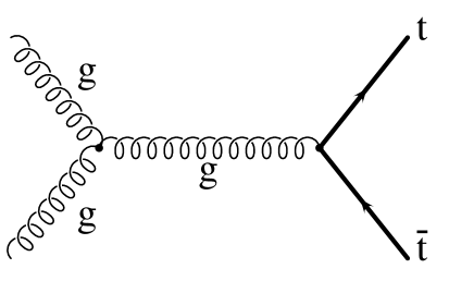
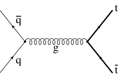
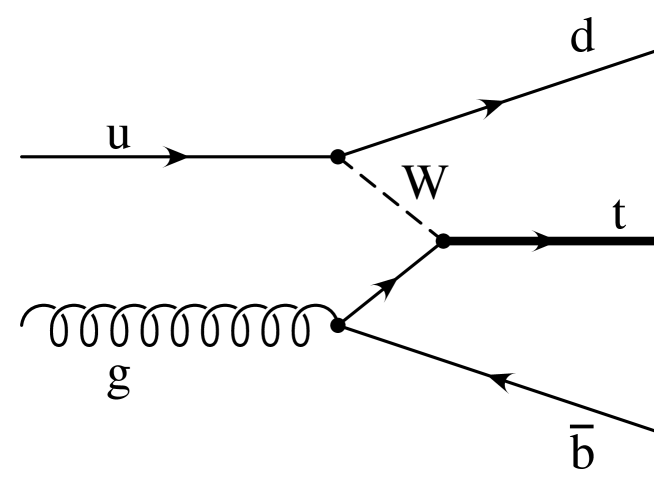
Figure 2.1: The main production mechanisms for top quarks in $p\overline{p}$ and $pp$ colliders [generic diagrams].

2.1 Lowest order predictions and qualitative features

The dominant Born terms for the total top cross section in $gg/\mbox{$q\overline{q}$}\mbox{$\rightarrow$ }\mbox{$t\overline{t}$}$ fusion are well-known to be of the form [55]

$$\sigma_{gg}(\hat{s})=\frac{4\pi\alpha^{2}_{s}}{12\hat{s}}\;\left[\;(1+\rho+\frac{\rho^{2}}{16})\;\ln\frac{1+\beta}{1-\beta}-\beta\;(\frac{7}{4}+\frac{31}{16}\rho)\;\right]\\$$

$$\sigma_{q\overline{q}}(\hat{s})=\frac{8\pi\alpha^{2}_{s}}{27\hat{s}}\;\beta\;[1+\frac{\rho}{2}]$$

with $\rho$ = 4$m_{t}^{2}/\hat{s}\;$ and $\beta=\sqrt{1-\rho}$ being the velocity of the $t$ quarks in the $t\overline{t}$ cm frame with invariant energy $\sqrt{\hat{s}}$. The total $p\bar{p}$ cross sections then follow by averaging the partonic cross sections over the $q\overline{q}$ and $gg$ luminosities in $p\bar{p}$ (and similarly in $pp$) collisions,

$$\sigma\left(p\bar{p}\mbox{$\rightarrow$ }\mbox{$t\overline{t}$}\right)=\int^{1}_{4m^{2}_{t}/s}d\tau\;\frac{d{\cal L}\left(gg\right)}{d\tau}\sigma_{gg}\left(\tau s\right)+\left[\mbox{$q\overline{q}$}\right]$$ (2.2)

The relative enhancement of the $q\bar{q}$ cross section by about a factor 3, as evident from the threshold behaviour

$$\sigma_{q\bar{q}} \approx {4\over 9}{\pi\alpha_{s}^{2}\over\hat{s}}\beta$$

$$\sigma_{gg} \approx {7\over 48}{\pi\alpha_{s}^{2}\over\hat{s}}\beta$$ (2.3)

has to be combined with the prominent $q\bar{q}$ luminosity at the TEVATRON.

Figure 2.2: Parton luminosities for TEVATRON and LHC energies.

Figure 2.3: Production cross section for $t\overline{t}$   pairs in $p\overline{p}$ and $pp$ colliders: Tevatron (1.8 GeV); Tevatron II (3.6 TeV); LHC (16 TeV); SSC (40 TeV). Ref.[44].

As shown in Fig. 2.2

$$\left.{\rm d}{\cal L}_{q\bar{q}}:{\rm d}{\cal L}_{gg}\right|_{\sqrt{\hat{s}}=2m}\approx\left\{\begin{array}[]{rl}5&{\rm TEVATRON}\\ 0.1&{\rm LHC}\end{array}\right.$$ (2.6)

which implies the dominance of $q\bar{q}$ annihilation, in contrast to the situation at the LHC, where gluon fusion is the dominant reaction.

A number of important features can be read off from this lowest order result:

• Since the parton luminosities rise steeply with decreasing $\tau$, the production cross sections increase dramatically with the energy (Fig. 2.3)

• Structure functions and quark-antiquark luminosities in the region of interest for the TEVATRON, i.e. for $\sqrt{\tau}$ between 0.2 and 0.4 are fairly well known from experimental measurements at lower energies (combined with evolution equations) and collider studies. The predictions are therefore quite stable with respect to variations between different sets of phenomenologically acceptable parton distributions. The near tenfold increase of the energy at the LHC and the corresponding decrease of $x$ and $\sqrt{\tau}$ by nearly a factor of ten leads to the dominance of gluon-gluon fusion and results in a significantly enhanced uncertainty in the production cross section.

• With the cross section proportional to $\alpha_{s}^{2}$ and uncertainties in $\alpha_{s}(M_{Z})$ which may be stretched up to $\pm 10\%$ one might naively expect a resulting uncertainty in the predicted cross section. However, the increase in the parton cross section with increasing $\alpha_{s}$ is, to some extent, compensated by a decrease in the parton luminosity (with increasing $\alpha_{s}$) for the kinematical region of interest at the TEVATRON. This compensation mechanism has been studied in [57] for inclusive jet production (Fig. 2.4) and applies equally well for top quark production.

• At the TEVATRON the rapidity distribution is strongly dominated by central production, $|y|\leq 1$, a consequence of the balance between the steeply falling proton and antiproton parton distributions. At the LHC, however, a rapidity plateau develops gradually and the distribution spans nearly four units in rapidity (Fig. 2.5).

  

  Figure 2.4: The $p\bar{p}$–initiated jet $E_{T}$ distribution at $\sqrt{s}=1.8$ TeV normalized to the prediction from partons with $\alpha_{S}=0.115$ (i.e. MRS.115). The data are the CDF measurements of $d^{2}\sigma/dE_{T}d\eta$ averaged over the rapidity interval $0.1<|\eta|<0.7$. The curves are obtained from a leading-order calculation evaluated at $\eta=0.4$. The data are preliminary and only the statistical errors are shown. The systematic errors are approximately 25% and are correlated between different $E_{T}$ points. (From [57]).

  Figure 2.5: Rapidity distribution of top quarks in $gg/q\bar{q}$ fusion at $\sqrt{s}=16$ TeV [44].

• The transverse momentum distribution is relatively flat, dropping down to half its peak value at around $p_{t}\approx m_{t}/2$, again a consequence of the competition between the increase of the phase space factor $\propto\beta$ in the parton cross section and the steeply decreasing parton luminosity (Fig. 2.6).

  Figure 2.6: The differential cross section for $p+\bar{p}\to t(\bar{t})+X$ with $m_{t}=120$ GeV/c² and $\mu_{R}=Q=\sqrt{m_{t}^{2}+p_{t}^{2}}$ at $\sqrt{s}=1.8$ TeV. The cross section is shown at different values of rapidity for (1) dashed lines: lowest order contribution scaled by an arbitrary factor (2) solid lines: full order $\alpha_{s}^{2}$ calculation. (From [58].)

  At the LHC the distribution will be even flatter and $p_{t}$ values around $2m_{t}$ are well within reach (Fig. 2.7). This corresponds to CMS energies between 0.5 and 1 TeV in the parton subsystem and extremely large subenergies are therefore accessible. This opens the possibility to search for the radiation of $W$, $Z$, or Higgs bosons in this reaction. For high energies the suppression of the cross section through electroweak virtual corrections (cf. sect. 2.2.3) is, at least partially, compensated by the large logarithm $\ln\hat{s}/M^{2}_{W,Z,H}$.

Figure 2.7: Transverse momentum distribution of top quarks in $gg/q\bar{q}$ at $\sqrt{s}=16$ TeV. (From [44].)

2.2 QCD and electroweak corrections

The observation of top quarks has been well established during the last year. One of the tools to study its properties, in particular its mass and its decay modes, is a precise experimental determination of its production cross section and subsequent decay in the $t\to b+W$ channel. A large deficiency in the comparison between theory and experiment would signal the presence of new decay modes which escape the canonical experimental cuts; with $t\to bH^{+}$ as most prominent example. However, the early round of experiments had indicated even an excess of top events when compared to the theoretical prediction for $m_{t}\approx 180$ GeV. This observation was difficult to interpret and the original calculations were scrutinized again by various authors. In particular, the resummation of leading logarithms and the influence of the Coulomb threshold enhancement was investigated — in the end, however, the prediction remained fairly stable.

In these lectures we will, therefore, in a first step, present the results from a complete NLO calculation (sect. 2.2.1). This is supplemented by a qualitative discussion of the resummation of higher order leading logarithmic terms. The influence of the Coulomb enhancement is studied in section 2.2.2, electroweak corrections are presented in sect. 2.2.3. Radiation of gluons may have a sizeable effect on the aparent mass of top quarks as observed in the experiment (sect. 2.2.4), with distinct differences between initial and final state radiation.

2.2.1 Next to leading order (NLO) corrections and resummation of large logarithms

Higher-order QCD corrections [59, 60, 58, 61] include loop corrections to the Born terms and $2\to 3$ contributions like $gg\to t\bar{t}g$, $q\bar{q}\to t\bar{t}g$ etc. For $q\bar{q}$ annihilation a few characteristic diagrams are displayed in Fig. 2.8. Real and virtual

                              (a)  (b)                 (c)  (d)

Figure 2.8: Initial and finite state radiation in the reaction $q\bar{q}\to t\bar{t}$

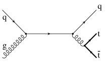
                       $$+\ldots$$

Figure 2.9: Reaction $qg\to t\bar{t}q$

initial state radiation (Fig. 2.8a,b) dominate, final state radiation from the slow top quarks (Fig. 2.8c) is unimportant, virtual gluon exchange at the $t\bar{t}$ vertex (Fig. 2.8d) leads to the Coulomb enhancement and will be discussed in sect. 2.2.2. The separation between $q\bar{q}$ annihilation and $qg$ reactions (Fig. 2.9) depends on the choice of the so-called factorisation scale $\mu^{2}$ which effectively enters the definition of the structure functions.

The differential as well as the total production cross section can be cast into the following form

$${\rm d}\sigma=\sum_{i,j=partons}\int{\rm d}x_{1}{\rm d}x_{2}F_{i}^{p}(x_{1},\mu^{2})F_{j}^{\bar{p}}(x_{2},\mu^{2}){\rm d}\sigma_{ij}\left(\hat{s},\ldots,\mu^{2}\right)$$ (2.7)

The renormalization scale $\mu_{R}$ and the factorisation scale $\mu_{F}$ are in general identified, $\mu_{R}=\mu_{F}\to\mu$, a matter of convention and convenience more than a matter of necessity. The parton distributions are extracted from structure functions as measured in deep inelastic scattering, and the analysis has to be taylored to the order of the calculation, i.e. to the NLO in the present case. The integrated expressions for the total cross sections can still be cast into a simple form

$$\sigma_{ij}(\hat{s},m_{t}^{2},\mu^{2})=\frac{\alpha_{s}^{2}(\mu^{2})}{m_{t}^{2}}\left[f_{ij}^{(0)}(\rho)+4\pi\alpha_{s}(\mu^{2})\left(f_{ij}^{(1)}(\rho)+\bar{f}_{ij}^{(1)}(\rho)\ln\frac{\mu^{2}}{m_{t}^{2}}\right)\right]$$ (2.8)

where $\hat{s}=x_{1}x_{2}s$ and the dominant lowest-order contributions $f^{(0)}_{ij}\left(\rho\right)$ are given by the parton cross sections above; in addition $f^{(0)}_{gq}=f^{(0)}_{g\bar{q}}=0$. The subleading higher-order expressions for $f^{(1)}_{ij}$ and $\bar{f}^{(1)}_{ij}$ are given in Refs.[59], [60]. The heavy quarks are treated within the on-shell renormalization scheme with $m_{t}$ being the ”physical” mass of the top quark. Outside the heavy quark sector, the $\overline{MS}$ scheme has been employed. These higher-order terms have to be used in conjunction with the running coupling $\alpha_{s}\left(\mu^{2}\right)$ and the gluon/light-quark parton densities evolved in 2-loop evolution equations. $\mu$ is the renormalization scale, identified here also with the factorization scale; typical scales that have been chosen are $\mu=m_{t}$ and $\sqrt{m^{2}_{t}+p^{2}_{T}}$. More technical details are discussed in Ref.[44].

The lowest- and higher-order predictions are compared with each other in Fig.2.3. In [44] it has been argued that the subdominant $2\mbox{$\rightarrow$ }3$ contributions add up to less than $10\%$ of the dominant lowest-order results. The theoretical uncertainties of the predictions for the LHC due to different parton distributions [62] were estimated about $\pm 10\%$ plus a $\pm 10\%$ variation due to the scale ambiguity $\mu$. The impact of the additional shift from the resummation of large logs arising in higher orders will be discussed below. Note that the ”K factor”, defined formally by the higher order corrections to the LO parton cross section, but the parton distributions and $\alpha_{s}$ kept fixed, amounts to an $\approx 50\%$ correction of the Born terms.

It is also instructive to study separate, physically distinct components of the $\alpha_{s}^{3}$ results [61]. The initial state bremsstrahlung (ISGB) processes, illustrated for the gluon initiated reactions in Fig.2.10, dominate

ISGB

FSGB

GS

FE

Figure 2.10: Generic QCD diagrams of the dominant higher order mechanisms.

around threshold [$\sqrt{\mbox{$\hat{s}$ }}\geq 2m_{t}$ or $p_{t}<m_{t})$], the case of relevance at the TEVATRON. The gluon splitting (GS) and the flavor excitation (FE) contributions become increasingly important for $\sqrt{\mbox{$\hat{s}$ }}\gg 2m_{t}$, the situation anticipated for the LHC.

Let us concentrate in the remainder of this section on the predictions for TEVATRON energies. Initial state radiation reduces the effective energy in the partonic subsystem, requiring larger initial parton energies to reach the threshold for top pair production. Considering the steeply falling parton distributions $F_{j}(x)$ one might, therefore, expect a reduction of $\sigma$ through NLO contributions. However, the same effect is operative in the very definition of $F_{j}$ (Fig. 2.11)

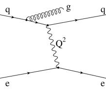
                              (a)  (b)

Figure 2.11: Definition of quark distributions, including NLO.

through deep inelastic scattering, including NLO corrections. In fact, without this compensation mechanism the result would not even be finite. However, the magnitude or even the sign of the correction cannot be guessed on an intuitive basis, and, not quite unexpected, even the precise form of $f^{(1)}$ and $\bar{f}^{(1)}$ depends on the definition of the structure functions. The most prominent examples are the $\overline{MS}$ scheme where $1/\epsilon$ poles (plus $\ln(4\pi)-\gamma$) from collinear singularities are simply dropped [more precisely, they are combined with the corresponding singular terms which arise in the NLO definition of the structure function] and finite corrections have to be applied when comparing to deep inelastic scattering, and the DIS scheme, where $F_{j}$ are defined through deep inelastic scattering to all orders.

Let us illustrate the qualitative aspects in the simpler example of NLO contributions to the Drell Yan process. The dominance of initial state radiation in the corrections to $t\bar{t}$ production will allow to apply the same reasoning to the case of interest in these lectures. Including NLO corrections one obtains

$${{\rm d}\sigma\over{\rm d}Q^{2}} = \sigma_{0}\sum_{i,j}\int_{0}^{1}{{\rm d}x_{i}\over x_{i}}{{\rm d}x_{j}\over x_{j}}F_{i}^{p}(x_{i},Q^{2})F_{j}^{\bar{p}}(x_{j},Q^{2})\cdot\omega_{ij}\left({\tau\over x_{i}x_{j}},\alpha_{s}\right)$$ (2.9)

$$= \sigma_{0}\sum_{i,j}\int_{\tau}^{1}{{\rm d}z\over z}{\cal F}_{ij}(\tau/z)\cdot\omega_{ij}(z,\alpha_{s})$$

with

$$\sigma_{0} \equiv {4\pi\alpha^{2}\over 9Q^{2}s}\qquad\qquad\qquad\tau\equiv{Q^{2}\over s}$$

$$\omega^{(0)}_{q\bar{q}}(z,\alpha_{s}) = e_{q}^{2}\delta(1-z)$$

$$\omega^{(1)}_{q\bar{q}}(z,\alpha_{s}) = e_{q}^{2}{\alpha_{s}\over 2\pi}C_{F}\left[2(1+z^{2})\left(\ln(1-z)\over 1-z\right)_{+}+3\left({1\over 1-z}\right)_{+}\right.$$ (2.10)

$$\left.\qquad+\left(1+{4\pi^{2}\over 3}\right)\delta(1-z)+\mbox{regular functions}\right]$$

(The quark-gluon induced reactions will not be discussed in this connection.) The plus prescription which regulates the singularity of the distributions at $z=1$ arises from the subtraction of collinear singularities. It can be understood by considering the limit

$$\left({\ln^{n}(1-z)\over 1-z}\right)_{+}\equiv\lim_{\epsilon\to 0}\left({\ln^{n}(1-z)\over 1-z}\Theta(1-\epsilon-z)+\delta(1-z){\ln^{n+1}\epsilon\over n+1}\right)$$ (2.11)

with the coefficient of the $\delta$ function adjusted such that the integral from zero to one vanishes.

Equivalently the plus-distribution can be defined through an integral with test functions $f(z)$. If $f(z)$ vanishes outside the interval $\langle\tau,1\rangle$ a convenient formula which will be of use below reads as follows

$$\int_{\tau}^{1}{\rm d}zf(z)\left({\ln^{n}(1-z)\over 1-z}\right)_{+}=\int_{\tau}^{1}{\rm d}z{f(z)-f(1)\over 1-z}\ln^{n}(1-z)-f(1)\int_{0}^{\tau}dz\,{\ln^{n}(1-z)\over 1-z}$$ (2.12)

The Born term $\omega^{(0)}$ is simply given by a $\delta$ function peak at $z=1$, corresponding to the requirement that the squared energy of the partonic system $\tau/z\times s$ and the squared mass of the muon pair $\tau\cdot s=Q^{2}$ be equal. ${\cal O}(\alpha_{s})$ corrections contribute to the $\delta$ function through vertex corrections and a continuous part from initial state radiation extending through the range

$$\tau\leq z\leq 1$$ (2.13)

The upper limit $z=1$ corresponds to the kinematic endpoint without radiation, the requirement $\tau\leq z$ originates from the fact that the parton luminoisities ${\cal F}_{ij}(\tau/z)$ vanish for $\tau/z>1$. The regular and the subleading pieces of $\omega$ are process dependent, the leading singularity $\sim(1+z^{2})\left({\ln(1-z)\over 1-z}\right)_{+}$ is universal (and closely related to the $q\to qg$ splitting function) and equally present in $t\bar{t}$ production.

The suppression of final state radiation in top pair production allows to extend the analogy to the Drell Yan process and to employ resummation techniques that were successfully developed and applied for muon pair production [63]. A complete treatment of this resummation is outside the scope of these lectures. Nevertheless we shall try to present at least qualitative arguments which allow to understand the origin of these large logarithms. (For a similar line of argument see [63].) With the energies of the partonic reaction $\sqrt{\hat{s}}={\cal O}(2-4m_{t})\approx 350-700$ GeV and the CMS energy $\sqrt{s}=1800$ GeV of comparable magnitude it is clear that the ratio $\hat{s}/s$ will not give rise to large logs. However, large logarithms can be traced to the interplay between the collinear singularity in the subprocess and the rapidly falling parton luminosity ${\cal F}_{ij}$ (cf. eq. (2.9)). This rapid decrease leads to a reduction in the effective range of integration. Let us, for the sake of argument assume a range reduced from

$$\tau\leq z\leq 1$$ (2.14)

to

$$1-\delta\leq z\leq 1$$ (2.15)

and evaluate the leading term. For a constant luminosity ${\cal F}(\tau/z)/z={\cal F}$ one would obtain

$$\int_{\tau}^{1}{\rm d}z\;2\left({\ln(1-z)\over 1-z}\right)_{+}{\cal F}=\ln^{2}(1-\tau){\cal F}$$ (2.16)

If the region of integration extended through the full kinematic range and with $\tau=4m_{t}^{2}/s=0.04$ there would be no large log. For the restricted range of integration, however, one finds

$$\int_{1-\delta}^{1}{\rm d}z\;2\left({\ln(1-z)\over 1-z}\right)_{+}{\cal F}=\ln^{2}(\delta){\cal F}$$ (2.17)

For small $\delta$, corresponding in practice to steeply falling luminosities one thus obtains large, positive (!) corrections from the interplay between ${\cal F}_{ij}(\tau/z)$ and $\omega_{q\bar{q}}$.

To arrive at a reliable prediction the leading terms of the form $(\alpha_{s}\ln^{2}\ldots)^{n}$ thus have to be included. The results are based on alternatively momentum space or impact parameter techniques which were originally developed for the Drell Yan process and applied to top pair production in [64]. An additional complication arises from the blow up of the coupling constant associated with the radiation of soft gluons for $\hat{s}\to 4m^{2}_{t}$. This has been interpreted in [64] as a breakdown of perturbation theory. Different regulator prescriptions have been advertised. In [64] a cutoff $\hat{s}-4m^{2}_{t}>\mu_{0}^{2}$ with $\mu^{2}_{0}\ll 4m^{2}_{t}$ was introduced to exclude a small fraction of the phase space.

The result is fairly stable for $q\bar{q}$ induced reactions with $\mu_{0}/m_{t}$ chosen between 0.05 and 0.2. The small contribution from gluon fusion, however, is sensitive towards $\mu_{0}$ which had to be chosen in the range between $0.2m_{t}$ and $0.3m_{t}$, a consequence of the enhancement of radiation from gluons. A slightly different approach (“principal value resummation”) has been advocated in [65] which circumvents the explicit $\mu_{0}$ dependence of the result, but leads essentially to the same final answer (Table 2.1).

$m_{t}$ [GeV]	175	180
$\mu_{0}$ (min)	4.72	3.86
$\mu_{0}$ (centr)	4.95	4.21
$\mu_{0}$ (max)	5.65	4.78
“principal value”	5.6	4.8

Table 2.1: Top production cross section (in pb) for $\sqrt{s}$ =1800 GeV for different values of the cutoff $\mu_{0}$ [64] (first three lines) and for the “principal value” prescription [65] (fourth line).

	$\sigma$ [pb]
Altarelli et al. [59]	$3.52$ (DFLM)
	$4.10$ (ELHQ)
Laenen et al. [64]	$\left.\begin{array}[]{ll}3.5&\quad(\mu^{2}=4m^{2})\\ 3.8&\quad(\mu^{2}=m^{2})\\ 4.05&\quad(\mu^{2}=m^{2}/4)\end{array}\right\}$ MRSD
Resummation
Laenen et al. [64]	$\left.\begin{array}[]{c}3.86\\ 4.21\\ 4.78\end{array}\right\}$ vary $\mu_{0}$
Berends et al. [66]	4.8 central value
Berger et al. [65]	4.8 “principal value res.”

Table 2.2: History of predictions for the production cross section for $\sqrt{s}=1.8$ TeV and $m_{t}=180$ GeV.

The result of the improved prediction (central value) is compared to the fixed order calculation (with $\mu^{2}=4m^{2},m^{2},m^{2}/4$) in fig. 2.12.

Figure 2.12: The NLO exact cross section as a function of the top quark mass for three choices of scale: $\mu=m/2$ (upper solid line), $\mu=m$ (central solid line) and $\mu=2m$ (lower solid line), and the NLO exact cross section plus the ${\cal O}(\alpha^{4}_{s})$ contribution at $\mu=m$ (dashed line) (from [64]).

Resummation evidently increases the cross section slightly above the previously considered range. The history of predictions is shown in table 2.2, with $\sqrt{s}=1.8$ TeV and $m_{t}=180$ GeV as reference values. The table demonstrates that the spread of predictions through a (fairly extreme) variation of structure functions (DFLM vs. ELHQ) and through a variation of the renormalisation and factorisation are comparable — typically around $\pm 10\%$. Leading log resummation increases the cross sections by $10-15\%$, with a sizeable sensitivity towards the cutoff prescription. A reduction in $m_{t}$ by 5 GeV leads to an increase of $\sigma$ by about 0.8 pb. Theory and experiment, with its present result of $7.6^{+2.4}_{-2.0}$ pb and $6.3\pm 2.2$ pb from CDF and D0 respectively are thus well compatible (Fig. 2.13).

Figure 2.13: Comparison of experimental results for the top quark mass and production cross section with the theoretical prediction.

2.2.2 Threshold behaviour

Near the $t\overline{t}$ threshold the cross sections are affected by resonance production and Coulomb rescattering forces [43], [67], [68]. These corrections can be estimated in a simplified potential picture. The driving one-gluon exchange potential is attractive if the $t\overline{t}$ is in color-singlet state and repulsive in a color-octet state [68],

$$\sigma^{(1)}(gg\mbox{$\rightarrow$ }t\overline{t}) = \frac{2}{7}\;\sigma_{B}(gg\mbox{$\rightarrow$ }t\overline{t})\mid\!\Psi^{(1)}\!\mid^{2}$$

$$\sigma^{(8)}(gg\mbox{$\rightarrow$ }t\overline{t}) = \frac{5}{7}\;\sigma_{B}(gg\mbox{$\rightarrow$ }t\overline{t})\mid\!\Psi^{(8)}\!\mid^{2}$$ (2.18)

$$\sigma^{(8)}(q\overline{q}\mbox{$\rightarrow$ }t\overline{t}) = \phantom{\frac{5}{7}}\;\sigma_{B}(q\overline{q}\mbox{$\rightarrow$ }t\overline{t})\mid\!\Psi^{(8)}\!\mid^{2}$$

with the correction factors (see fig. 2.14) given in NLO by

$$\beta|\psi|^{2}=\beta\left(1+{\pi\alpha_{s}\over 2\beta_{t}}\left\{\begin{array}[]{cc}4/3&\mbox{singlet}\\ -1/6&\mbox{octet}\end{array}\right.\right)$$ (2.21)

The summation of the leading $\pi\alpha_{s}/\beta$ terms to all orders results in the familiar Sommerfeld correction factor

$$\beta|\psi|^{2}=\beta{x\over 1-e^{-x}}$$ (2.22)

For $t\bar{t}$ in the singlet configuration $x=x^{(1)}\equiv{4\over 3}{\pi\alpha_{s}\over\beta}$, for octet states $x=x^{(8)}\equiv-{1\over 6}{\pi\alpha_{s}\over\beta}$.

The Coulombic attraction thus leads to a sharp rise of the cross section at the threshold in the singlet channel, even if no resonance can be formed anymore, since the phase space suppression of the Born term $\sigma_{B}\propto\beta_{t}$ is neutralized by the Coulomb enhancement of the wave function $\left|\Psi_{1}\right|^{2}\propto\alpha_{s}/\beta$. In the octet channel (dominant for $q\bar{q}$ annihilation), by contrast, the cross sections are strongly reduced by the Coulombic repulsion which leads effectively to an exponential fall-off of the cross sections $\sigma_{8}\propto\exp\left[-\pi\alpha_{s}/6\beta_{t}\right]$ at the threshold [68]. Due to the averaging over parton luminosities the effects are less spectacular in $p\bar{p}$ or $pp$ than in $e^{+}e^{-}$ collisions.

The enhancement and suppression factors are compared to simple phase space $\sim\beta$ in Fig. 2.17.

	$\sim\beta_{t}$
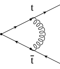
	$\sim\beta_{t}\cdot{\pi\alpha_{s}\over 2\beta_{t}}\left\{\begin{array}[]{ll}4/3&{\rm singlet}\\ -1/6&{\rm octet}\end{array}\right.$

Figure 2.14: Vertex corrections from gluon exchange in the threshold region.

The dotted line corresponds to the phase space factor $\beta$, the dashed line to the perturbative NLO calculation (2.21), the solid line to the Coulomb enhancement given in eq. (2.22). The predictions for the singlet, octet ($\equiv q\bar{q}$), and properly weighted gluon fusion channel are displayed in Figs. 2.17 a, b, and c, respectively.

Figure 2.15: Threshold enhancement and suppression factors for singlet (upper), octet (middle), and properly weighted gluon fusion (lower figure) for $\alpha_{s}=0.15$. Dotted line: Born approximation; dashed line: NLO approximation; solid line: Coulomb enhancement.

2.2.3 Electroweak corrections

Another potentially important modification which is closely tied to the Coulomb enhancement originates from vertex corrections induced by light Higgs boson exchange. In a simplified treatment these are lumped into a Yukawa potential

$$V(r)={\sqrt{2}G_{F}m_{t}^{2}\over 4\pi}{e^{-m_{H}r}\over r}$$ (2.23)

resulting in a reduction $\delta E$ of the apparent threshold, with $\delta E=-200$ MeV for $m_{H}=100$ GeV as characteristic example. The change in the normalisation by $+10\%$ could become relevant for precision measurements. The situation is quite similar to the one discussed for $e^{+}e^{-}$ colliders in section 3.2.

Genuine electroweak contributions of ${\cal O}\left(\alpha\alpha^{2}_{s}\right)$ have been calculated to both the $q\overline{q}$ and $gg\mbox{$\rightarrow$ }\mbox{$t\overline{t}$}$ subprocesses [69]. The corrections include vertex corrections and box diagrams built-up by vector bosons and the Higgs boson (Fig. 2.16).

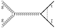
Figure 2.16: Feynman diagrams contributing to the electroweak radiative corrections. Dashed lines stand for $H$, $Z$, $\gamma$, or $W$.

Figure 2.17: Relative correction to the parton cross section for $m_{t}=250$ GeV (upper figure: $q\bar{q}\to t\bar{t}$, lower figure: $gg\to t\bar{t}$) (from [69]).

Except for a small region close to the production threshold, which is dominated by the Yukawa potential, the corrections are always negative; they can become sizeably large, in particular if the top is very heavy and if the energy of the subsystem exceeds 1 TeV, not uncommon for $t\bar{t}$ production at the LHC. In this case however, the large negative corrections are compensated by positive contributions from real radiation of $W$, $Z$, or $H$. The corrections for the $q\bar{q}$ and $gg$ subprocess as functions of the parton energies are shown in Fig. 2.17. The sharp increase of the corrections close to threshold for a light Higgs is clearly visible and, similarly, the large negative correction for large parton energies. After convoluting the cross sections of the subprocesses with the parton distributions, a reduction of the Born cross section at a level of a few percent is observed (Fig. 2.18).

Figure 2.18: Relative correction to the hadronic cross section for $s=(16$ TeV)² (from [69])

2.2.4 Gluon radiation

Up to this point the discussion has centered around the predictions for inclusive top quark production. Additional ingredients for the experimental analysis are the detailed topological structure of the signal, the number of jets, the characteristics of the underlying event, and, of course, predictions for the background. This information allows to adjust in an optimal way experimental cuts and to measure the top quark through a kinematic analysis of its decay products. As a typical example the impact of gluon radiation on the top mass determination has been analysed recently. An idealized study has been performed e.g. in [70]. Radiated gluons are merged with the $b$ jet from top decay or with the quark jet from $W\to q\bar{q}$ if they are found within a cone of opening angle

$$R=\sqrt{(\Delta\eta)^{2}+(\Delta\phi)^{2}}<R_{cut}$$ (2.24)

with respect to $b$, $q$ or $\bar{q}$ and if their rapidity is below $|\eta|<2$. In this case the gluon is considered as top decay product and hence contributes to its invariant mass. If the gluon jet falls outside the cuts, it is assigned the rest of the event.

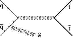
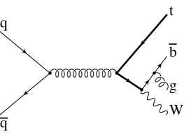
Figure 2.19: Gluon radiation from top production (upper) and decay (lower diagrams).

Gluon radiation associated with top quark production, if erroneously associated with top decay, will thus increase the apparent $m_{t}$. Radiation from top decay, if outside the forementioned cuts, will however, decrease the measured mass of the quark. The interplay between the two compensating effects is displayed in Fig. 2.20.

Figure 2.20: Shift in the apparent top mass as a function of $R$ cut (from [70]).

For a realistic $R_{cut}\approx 0.6$ a reduction $\Delta m$ of around 2 GeV is predicted.

2.3 Single top production

Virtual $W$ bosons, originating from $u\to dW$ splitting, can merge with bottom quarks from gluon splitting $g\to b\bar{b}$ to produce single top quarks in association with fairly collinear $d$- and $\bar{b}$- jets (Fig. 2.21).

             

Figure 2.21: Characteristic diagram for single top production.

The interaction radius in the QCD $gg$ fusion process shrinks with rising energy so that the cross section $\sigma(gg\rightarrow\mbox{$t\overline{t}$ })\sim\alpha_{s}^{2}/\mbox{$\hat{s}$ }$ [mod. log’s] vanishes asymptotically. By contrast, the interaction radius in the weak fusion process [56] is set by the Compton wave length of the $W$ boson and therefore asymptotically non-zero, $\sigma\rightarrow G_{F}^{2}m_{W}^{2}/2\pi$. The subprocess has to be folded with the quark-gluon luminosities

$$\sigma(p\bar{p}\to t+X)=\int_{\tau}^{1}{{\rm d}z\over z}{\cal L}_{ug}(\tau/z)\sigma(ug\to t+\bar{b}+d)$$ (2.25)

plus a similar contribution from $\bar{d}g\to t+\bar{b}+\bar{u}$. The fall-off of the total cross section $\sigma(pp\rightarrow t\overline{b})$ is less steep than for the QCD fusion processes. As a result, the $Wg$ fusion process would have dominanted for large top quark masses $\geq$ 250 GeV at the LHC (Fig. 2.23).

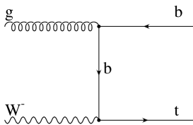
(a)	(b)

Figure 2.22: Characteristic diagrams for top production via Compton scattering (a) and Drell Yan process (b)

For $m_{t}=$ 180 GeV, the case of practical interest, single top production is about a factor 5 below the QCD reaction. Nevertheless, as shown in Fig.2.23, about 10⁶ top quarks will be produced at the LHC by this mechanism at an integrated luminosity of $\int\cal L$ = 10${}^{4}pb^{-1}$. Also at the TEVATRON this process should be accessible with the anticipated luminosity.

Figure 2.23: Cross sections for several mechanisms of top quark production [44]. Various parametrizations and models of the parton densities [62] have been used.

A close inspection of the various contributions to the subprocess $ug\to t+\bar{b}+d$ reveals immediately that the by far dominant part of the cross section is due to $b$ exchange, with the b quark being near its mass shell. Since the $b$ quark is almost collinear to the incoming gluon, this cross section is logarithmically enhanced $\sim\ln(m_{t}^{2}/m_{b}^{2})$ over other mechanisms. This naturally suggests to approximate the process by the subprocess $u$ + $b$ $\stackrel{{\scriptstyle\mbox{\scriptsize W}}}{{\rightarrow}}$ $d$ + $t$ with the $b$-quark distribution generated perturbatively by gluon splitting based on massless evolution equations. The weak cross sections can be presented in a compact form,

$$\sigma(ub\stackrel{{\scriptstyle\mbox{\scriptsize W}}}{{\rightarrow}}dt) = \frac{G_{F}^{2}m_{W}^{2}}{2\pi}\;\frac{(\mbox{$\hat{s}$ }-m_{t}^{2})^{2}}{\mbox{$\hat{s}$ }(\mbox{$\hat{s}$ }+m_{W}^{2}-m_{t}^{2})}\mbox{\hskip 142.26378pt }\rightarrow\frac{G_{F}^{2}m_{W}^{2}}{2\pi}$$

$$\sigma(d\overline{b}\stackrel{{\scriptstyle\mbox{\scriptsize W}}}{{\rightarrow}}u\overline{t}) \rule[-2.84526pt]{0.0pt}{28.45274pt}= \frac{G_{F}^{2}m_{W}^{2}}{2\pi}\;\left[\;1+\frac{\mbox{$\hat{s}$ }(2m_{W}^{2}-m_{t}^{2})-2m_{W}^{2}m_{t}^{2}}{\mbox{$\hat{s}$ }^{2}}\right.$$

$$\mbox{\hskip 45.52458pt}\left.-\;\frac{(2\mbox{$\hat{s}$ }+2m_{W}^{2}-m_{t}^{2})m_{t}^{2}}{\mbox{$\hat{s}$ }^{2}}\;\log\frac{\mbox{$\hat{s}$ }+m_{W}^{2}-m_{t}^{2}}{m_{W}^{2}}\;\right]\mbox{}\rightarrow\frac{G_{F}^{2}m_{W}^{2}}{2\pi}$$

and identically the same expressions for the $\cal C$-conjugate reactions.

Top quarks are created in $u+g$ collisions, anti-top quarks in $d+g$ collisions where the absorption of a $W^{-}$ transforms a $\overline{b}$ quark to a $\overline{t}$ quark. The na$\ddot{\mbox{\i}}$ve expectation from valence quark counting for the ratio of $t/\overline{t}$ cross sections, $\sigma(u\rightarrow t):\sigma(d\rightarrow\overline{t})$ $\sim$ 2 : 1 is corroborated by a detailed analysis; in fact, the ratio turns out to be 2.1 for top quark masses of about 150 GeV.

The remaining possibilities for single top production are Compton scattering (Fig. 2.22(a))

$$g+b\to W+t$$ (2.26)

and the Drell Yan process (Fig. 2.22(b))

$$u+\bar{d}\to t+\bar{b}$$ (2.27)

The predicted cross sections are too small to be of practical interest. Single top quark production via the dominant mechanism (Fig. 2.21) offers a unique way for a measurement of the CKM matrix element $V_{tb}$ and thus, indirectly of the top quark life time. As discussed in section 1.2.1 $V_{tb}$ is strongly constrained to be very close to one for three generations — in a four generation model $V_{tb}$ may be quite different from these expectations.

2.4 Quarkonium production

Both charm and bottom quarks have been discovered at hadron colliders in the form of quarkonium resonances $J/\psi$ and $\Upsilon$ through their distinct signals in the $\mu^{+}\mu^{-}$ channel. The search for toponium at a hadron collider is, however, entirely useless. The broad ($\Gamma\sim$ 2 GeV) resonances decay with an overwhelming probability through single quark decay and are therefore indistinguishable from open top quarks produced close to threshold.

The situation could be different in extensions of the SM. Decays of a fourth generation $b^{\prime}$

$$b^{\prime}\to t+W$$ (2.28)

are suppressed by small mixing angles. Alternatively, if $m_{b^{\prime}}<m_{t}+m_{W}$, the $b^{\prime}\to c+W$ mode would have to compete with loop induced FCNC decays — leaving ample room for narrow quarkonium states. Another example would be the production of weak isosinglet quarks which are predicted in Grand Unified Theories. The decay of these quarks would again be inhibited by small mixing angles.

Of particular interest is the search for $\eta_{b^{\prime}}$, the ${}^{1}S_{0}$ state composed of $b^{\prime}$ and $\bar{b}^{\prime}$ [71, 72, 73]. It is produced with appreciable cross section. Its dominant decay mode

$$\eta_{b^{\prime}}\to H+Z$$ (2.29)

is enhanced by the large Yukawa coupling, governing the coupling of the heavy quark to the Higgs and the longitudinal $Z$. For large $m_{b^{\prime}}$ one obtains

$${\Gamma(\eta_{b^{\prime}}\to H+Z)\over\Gamma(\eta_{b^{\prime}}\to\gamma\gamma)}\sim{m_{b^{\prime}}^{4}\over M_{W}^{4}}$$ (2.30)

The branching ratios as functions of $M_{\eta}$ are displayed in Fig. 2.24.

Figure 2.24: Branching ratios of $\eta_{b^{\prime}}$ for the dominant decay modes as functions of the bound state mass $M$.

The complete set of QCD corrections for leading and subleading annihilation decay modes can be found in [73]. They do not alter the picture significantly.

It should be emphasized that the decay $\eta_{b^{\prime}}\to H+Z$ proceeds through the axial part of the neutral current coupling which, in turn, is proportional to the third component of the weak isospin. Bound states of isosinglet quarks would, therefore, decay dominantly into two gluon jets.

The cross section for open $b\bar{b}^{\prime}$ production at the LHC (with $m_{b^{\prime}}=300$ GeV) amounts to about 100 pb. The fraction of the phase space where bound states can be formed, i.e. for relative quark velocity $\beta<0.1$, covers around $10^{-2}$ of the relevant region

$${\int_{0}^{0.1}{\rm d}\beta\beta\over\int_{0}^{1}{\rm d}\beta\beta}=10^{-2}$$ (2.31)

and indeed one predicts a production cross section somewhat less than 1 pb from a full calculation.

For a detailed calculation of the production cross section a proper treatment of the QCD potential is required to obtain a reliable prediction for the bound state wave function at the origin. The structure of the NLO corrections for the production cross section, in particular of the dominant terms, bears many similarities with the result for open production and for the Drell Yan process (eq. 2.10). For gluon fusion the partonic cross section is (in the $\overline{MS}$ scheme) given by [74, 75]

$$\hat{\sigma}^{gg}={1\over s}{\pi^{2}\over 3}{R^{2}(0)\over M^{3}}\alpha^{2}_{\overline{\rm MS}}(M^{2})\left\{\rule{0.0pt}{14.22636pt}\delta(1-z)\right.$$

$$\left.+{\alpha_{\overline{\rm MS}}(M^{2})\over\pi}\left\langle\delta(1-z)\left(N_{C}\left(1+{\pi^{2}\over 12}\right)C_{F}\left({\pi^{2}\over 4}-5\right)-{4\over 3}T_{f}\ln(2)\right)+N_{C}F(z)\right\rangle\right\}$$

where

$$F(z) = \Theta(1-z)\left[{11z^{5}+11z^{4}+13z^{3}+19z^{2}+6z-12\over 6z(1+z)^{2}}\right.$$ (2.33)

$$+4\left({1\over z}+z(1-z)-2\right)\ln(1-z)+4\left({\ln(1-z)\over 1-z}\right)_{+}$$

$$\left.+\left({2(z^{3}-2z^{2}-3z-2)(z^{3}-z+2)z\ln(z)\over(1+z)^{3}(1-z)}-3\right){1\over 1-z}\right]$$

and $z=M^{2}/{\hat{s}}$. Both Born term and the virtual correction are proportional to $\delta(1-z)$, the structure of the dominant term due to gluon splitting $\sim\ln(1-z)/(1-z)$ is again universal. Quark-gluon and quark-antiquark initiated subprocesses of order $\alpha^{3}_{s}$ can be found in [74, 75]. It may be worth mentioning that the structure of QCD corrections to light Higgs production [76] is nearly identical to eq. LABEL:eq:ttp9235. From Fig. 2.25 it is evident that $\eta_{b^{\prime}}$ states with masses up to 1 TeV are produced at the LHC with sizeable rates. The fairly clean signature of the $Z+H$ decay mode might allow to discover these exotic quarkonia and the Higgs boson at the same time.

Figure 2.25: Production cross section for $\eta_{b^{\prime}}$ including QCD corrections as function of the bound state mass $M$ for $\sqrt{s}=16$ TeV and 40 TeV.

Chapter 3 Top quarks in $e^{+}e^{-}$ annihilation

A variety of reactions is conceivable for top quark production at an electron positron collider. Characteristic Feynman diagrams are shown in Fig.3.1. $e^{+}e^{-}$ annihilation through the virtual photon and $Z$ (Fig.3.1a) dominates and constitutes the reaction of interest for the currently envisaged energy region.

Figure 3.1: Feynman diagrams for $t\bar{t}$ or $t\bar{b}$ production.

In addition one may also consider [77] a variety of gauge boson fusion reactions (Fig.3.1b-d) that are in close analogy to $\gamma\gamma$ fusion into hadrons at $e^{+}e^{-}$ machines of lower energy. Specifically these are single top production,

$$e^{+}e^{-}\to\bar{\nu}e^{-}t\bar{b}$$ (3.1)

or its charge conjugate and top pair production through neutral or charged gauge boson fusion

$$e^{+}e^{-} \to e^{+}e^{-}t\bar{t}$$

$$e^{+}e^{-} \to \bar{\nu}\nu t\bar{t}$$ (3.2)

The experimental observation of these reactions would allow to determine the coupling of top quarks to gauge bosons, in particular also to longitudinal $W$ bosons and $Z$ bosons, in the space-like region and eventually at large momentum transfers. This would constitute a nontrivial test of the mechanism of spontaneous symmetry breaking.

The various cross sections increase with energy in close analogy to $\gamma\gamma$ reactions, and eventually even exceed $e^{+}e^{-}$ annihilation rates. However, at energies accessible in the foreseeable future these reactions are completely negligible: for an integrated luminosity of $10^{40}$ cm^-2, at $E_{cm}=500~{}GeV$ and for $m_{t}=150~{}GeV$ one expects about one $e^{+}e^{-}t\bar{t}$ event (still dominated by $\gamma\gamma$ fusion). At that same energy the cross sections for $e^{+}\nu\bar{t}b+c.c.$ and $\nu\bar{\nu}t\bar{t}$ final states are still one to two orders of magnitude smaller.

Another interesting class of reactions is $e^{+}e^{-}$ annihilation into heavy quarks in association with gauge or Higgs bosons:

$$e^{+}e^{-} \to t\bar{t}Z$$ (3.3)

$$e^{+}e^{-} \to t\bar{b}W^{-}$$ (3.4)

$$e^{+}e^{-} \to t\bar{t}H$$ (3.5)

$$e^{+}e^{-} \to t\bar{b}H^{-}$$ (3.6)

Two amplitudes contribute to the first reaction [78]: The $t\bar{t}$ system may be produced through a virtual Higgs boson which by itself was radiated from a $Z$ (Fig.3.2). The corresponding amplitude dominates the rate and provides a direct measurement of the Yukawa coupling. The radiation of longitudinal $Z$’s from the quark line in principle also carries information on the symmetry breaking mechanism of the theory.

Figure 3.2: Amplitudes relevant for $e^{+}e^{-}\to t\bar{t}Z$ and for $e^{+}e^{-}\to t\bar{t}H$.

The transverse part of the $t\bar{t}Z$ coupling, i.e. the gauge part, can be measured directly through the cross section or various asymmetries in $e^{+}e^{-}\to t\bar{t}$. The longitudinal part, however, could only be isolated with $t\bar{t}Z$ final states. For an integrated luminosity of $10^{40}$ cm^-2 one expects only about 40 events (see sect. 3.1.7) and it is therefore not clear whether these can be filtered from the huge background and eventually used for a detailed analysis.

Light Higgs bosons may be produced in conjunction with $t\bar{t}$ [79]. They are radiated either from the virtual $Z$ with an amplitude that is present also for massless fermions or directly from heavy quarks as a consequence of the large Yukawa coupling (Fig.3.2). The latter dominates by far and may therefore be tested specifically with heavy quark final states. The predictions for the rate will be discussed in sect. 3.1.7. Depending on the mass of the Higgs and the top quark, the reaction could perhaps be detected with an integrated luminosity of $10^{40}cm^{-2}$.

Top quark production in $\gamma\gamma$ collisions is conceivable at a “Compton collider”. It requires special experimental provisions for the conversion of electron beams into well-focused beams of energetic photons through rescattering of laser light. A detailed discussion can be found in [80].

Chapter 3 will be entirely devoted to $t\bar{t}$ production in $e^{+}e^{-}$ annihilation. Section 3.1 will be concerned with the energy region far above threshold — with electroweak aspects as well as with specific aspects of top hadronisation. The emphasis of section 3.2 will be on the threshold region which is governed by the interplay between bound state formation and the rapid top decay.

3.1 Top production above threshold

3.1.1 Born predictions

From the preceding discussion it is evident that the bulk of top studies at an $e^{+}e^{-}$ collider will rely on quarks produced in $e^{+}e^{-}$ annihilation through the virtual $\gamma$ and Z, with a production cross section of the order of $\sigma_{point}$. For quarks tagged at an angle $\vartheta$, the differential cross section in Born approximation is a binomial in $\cos\vartheta$

$$\frac{d\sigma}{d\cos\vartheta}=\frac{3}{8}\left(1+\cos^{2}\vartheta\right)\sigma_{U}+\frac{3}{4}\sin^{2}\vartheta\sigma_{L}+\frac{3}{4}\cos\vartheta\sigma_{F}$$ (3.7)

$U$ and $L$ denote the contributions of unpolarized and longitudinally polarized gauge bosons along the $\vartheta$ axis, and $F$ denotes the difference between right and left polarizations. The total cross section is the sum of $U$ and $L$,

$$\sigma=\sigma_{U}+\sigma_{L}$$ (3.8)

the forward/backward asymmetry is given by the ratio

$$A^{FB}=\frac{3}{4}\frac{\sigma_{F}}{\sigma}$$ (3.9)

The $\sigma^{i}$ can be expressed in terms of the cross sections for the massless case in Born approximation,

$$\sigma^{U}_{B} = \beta\sigma^{VV}+\beta^{3}\sigma^{AA}$$

$$\sigma^{L}_{B} = \frac{1}{2}\left(1-\beta^{2}\right)\beta\sigma^{VV}$$

$$\sigma^{F}_{B} = \beta^{2}\sigma^{VA}$$ (3.10)

with

$$\sigma^{VV} = \frac{4\pi\alpha^{2}(s)e^{2}_{e}e^{2}_{Q}}{s}$$

$$+\frac{G_{F}(s)}{\sqrt{2}}e_{e}e_{Q}(\upsilon_{e}+\rho a_{e})\upsilon_{Q}\frac{m^{2}_{Z}\left(s-m^{2}_{Z}\right)}{\left(s-m^{2}_{Z}\right)^{2}+\left(\frac{s}{m_{Z}}\Gamma_{Z}\right)^{2}}$$

$$+\frac{G^{2}_{F}}{32\pi}\left(\upsilon^{2}_{e}+a^{2}_{e}+2\rho\upsilon_{e}a_{e}\right)\upsilon^{2}_{Q}\frac{m^{4}_{Z}s}{\left(s-m^{2}_{Z}\right)^{2}+\left(\frac{s}{m_{Z}}\Gamma_{Z}\right)^{2}}$$

$$\sigma^{AA} = \frac{G^{2}_{F}}{32\pi}\left(\upsilon^{2}_{e}+a^{2}_{e}+2\rho\upsilon_{e}a_{e}\right)a^{2}_{Q}\frac{m^{4}_{Z}s}{\left(s-m^{2}_{Z}\right)^{2}+\left(\frac{s}{m_{Z}}\Gamma_{Z}\right)^{2}}$$

$$\sigma^{VA} = \frac{G_{F}\alpha(s)}{\sqrt{2}}e_{e}(\rho\upsilon_{e}+a_{e})e_{Q}a_{Q}\frac{m^{2}_{Z}\left(s-m^{2}_{Z}\right)}{\left(s-m^{2}_{Z}\right)^{2}+\left(\frac{s}{m_{Z}}\Gamma_{Z}\right)^{2}}$$ (3.11)

$$+\frac{G^{2}_{F}}{16\pi}\left(2\upsilon_{e}a_{e}+\rho(\upsilon^{2}_{e}+a^{2}_{e})\right)\upsilon_{Q}a_{Q}\frac{m^{4}_{Z}s}{\left(s-m^{2}_{Z}\right)^{2}+\left(\frac{s}{m_{Z}}\Gamma_{Z}\right)^{2}}$$

The fermion couplings are given by

$$\upsilon_{f}=2I^{f}_{3}-4e_{f}\sin^{2}\theta_{w}\quad,\qquad a_{f}=2I^{f}_{3}$$ (3.12)

and the possibility of longitudinal electron polarization ($\rho=-1;+1;0$ for righthanded; lefthanded; unpolarized electrons) has been included. Alternatively one may replace $G_{F}m^{2}_{Z}$ by

$$G_{F}m^{2}_{Z}=\frac{\pi\alpha(s)}{\sqrt{2}\sin^{2}\theta_{W}\cos^{2}\theta_{W}}$$ (3.13)

With $\sin^{2}\theta_{W}$ ($\approx$0.23) interpreted as $\sin^{2}\theta_{eff}$ [81] this formula accommodates the leading logarithms from the running coupling constant as well as the quadratic top mass terms in the threshold region.

3.1.2 Radiative corrections

QCD corrections to this formula are available for arbitrary $m^{2}/s$ up to first order in $\alpha_{s}$:

$$\sigma = \frac{(3-\beta^{2})}{2}\beta\sigma^{VV}\left(1+\frac{4}{3}\frac{\alpha_{s}}{\pi}K_{V}\right)$$ (3.14)

$$+\beta^{3}\sigma^{AA}\left(1+\frac{4}{3}\frac{\alpha_{s}}{\pi}K_{A}\right)$$

The exact result [82] for $K_{V,A}$ can be found in [83]. These QCD enhancement factors are well approximated by [84]

$$K_{V} = 1+\frac{4}{3}\alpha_{s}\left[\frac{\pi}{2\beta}-\frac{3+\beta}{4}\left(\frac{\pi}{2}-\frac{3}{4\pi}\right)\right]$$

$$K_{A} = 1+\frac{4}{3}\alpha_{s}\left[\frac{\pi}{2\beta}-\left(\frac{19}{10}-\frac{22}{5}\beta+\frac{7}{2}\beta^{2}\right)\left(\frac{\pi}{2}-\frac{3}{4\pi}\right)\right]$$

$$\alpha_{s} = \frac{12\pi}{25\log(4p^{2}_{t}/\Lambda^{2})}$$ (3.15)

The next to leading order corrections to $K_{V}$ were calculated only recently [85, 86]. The scale in $\alpha_{s}$ chosen above was guessed on the basis of general arguments [67] which were confirmed by the forementioned complete calculations.

For small $\beta$ these factors develop the familiar Couloumb enhancement $\sim{2\pi\alpha_{s}\over 3\beta}$, compensating the phase space $\sim\beta$. This leads to a nonvanishing cross section which smoothly joins the resonance region. Details of this transition will be treated in section 3.2.

To prepare this discussion, let us briefly study the limit of applicability of fixed order perturbation theory. The leading terms in the perturbative expansion close to threshold are obtained from Sommerfeld’s rescattering formula $\left(x\equiv{4\over 3}{\pi\alpha\over\beta}\right)$

$$K_{V}^{\rm Som}={x\over 1-e^{-x}} = 1+{x\over 2}+{B_{1}x^{2}\over 2!}-{B_{2}x^{4}\over 4!}+{B_{3}x^{6}\over 6!}\pm\ldots$$ (3.16)

$$= 1+{x\over 2}+{x^{2}\over 12}-{x^{4}\over 720}+{x^{6}\over 5040}\pm\ldots$$

with $B_{i}$ being the Bernoulli numbers. At first glance one might require $x\leq 1$ for the perturbative expansion to be valid. However, significantly larger values of $x$ are acceptable. The full Sommerfeld factor $K_{V}^{\rm Som}$ is remarkably well approximated by the first three terms of the series for surprisingly large $x$ (only 6% deviation for $x=4!$). For top quarks this corresponds to $\beta\approx 0.13-0.14$ and hence down to about 3 GeV above the nominal threshold. Upon closer inspection one also observes that the formula given in eq. (3.15) (a result of order $\alpha_{s}$) coincides numerically well with the correction factor $K_{V}^{\rm Som}\left(1-{16\over 3}{\alpha_{s}\over\pi}\right)$ which incorporates rescattering and hard gluon vertex corrections. The results presented in these lectures are based on the Born predictions plus ${\cal O}(\alpha_{s})$ corrections.

Initial state radiation has an important influence on the magnitude of the cross section. $\sigma(s_{eff})$ is folded with the Bonneau Martin structure function, supplemented by the summation of large logarithms. A convenient formula for the non-singlet structure function in the leading logarithmic approximation has been obtained in [87], which is a natural extension of a formula proposed in [88]. This leads to a significant suppression by about a factor

$$\left(\frac{\delta W}{m_{t}}\right)^{{2\alpha\over\pi}\left(\ln{m_{t}^{2}\over m_{e}^{2}}-1\right)}\approx 0.5-0.6$$ (3.17)

with $\delta W=1-5~{}GeV$ in the resonance and threshold region. The correction factor increases rapidly with energy, but stays below 0.9 in the full range under consideration (Fig.3.3).

Electroweak corrections to the production cross section in the continuum have been studied in [89]. Apart from a small region close to threshold they are negative. Relative to the $G_{F}$ parametrized Born approximation they decrease the cross section by -6.3% to -9.3%, if $m_{t}$ is varied between 100 and 200 GeV, $m_{H}$ between 42 and 1000 GeV, and $E_{cm}$ fixed at 500 GeV. QCD and electroweak corrections are thus of equal importance (Fig. 3.4).

Close to threshold and for relatively small Higgs boson masses a rapid increase of these corretions is observed (Fig. 3.5) which can be attributed to the attractive Yukawa potential induced by light Higgs boson exchange. Several GeV above threshold, and for $m_{H}$ around or below 100 GeV it is more appropriate to split these corrections into hard and soft exchange and incorporate the latter in an instantaneous Yukawa potential [90].

Figure 3.3: Cross section for $t\bar{t}$ production, including resonances, QCD corrections and initial state radiation in units of $\sigma_{point}$.

Figure 3.4: Genuine electroweak corrections to top production in $e^{+}e^{-}$ annihilation. From [89].

Figure 3.5: Relative size (in percent) of electroweak corrections in the threshold region for $m_{t}=200$ GeV and different Higgs masses (from [91]).

Longitudinal polarization

It should be mentioned that linear colliders might well operate to a large extent with polarized (electron) beams. The cross section for this case can be derived from (3.11). For top quarks the resulting right/left asymmetry

$$A_{LR}=(\sigma_{L}-\sigma_{R})/(\sigma_{L}+\sigma_{R})$$ (3.18)

is sizable (Fig.3.6) and amounts to about $-\,0.4$,

Figure 3.6: Right/left asymmetry as function of $E_{cm}$ for $m_{t}=150~{}GeV$.

reducing the production cross section with righthanded electrons. However, selection of righthanded electron beams decreases the $W$ pair cross section even stronger, thereby enhancing the top quark signal even before cuts are applied. Electroweak corrections to $A_{LR}$ in the threshold region have been calculated in [92].

3.1.3 Top quark fragmentation

The experimental analysis of charm and bottom fragmentation functions has clearly demonstrated that heavy quark fragmentation is hard in contrast to the fragmentation of light quarks. This is a consequence of the inertia of heavy particles, the momentum of which is not altered much if a light quark $\bar{q}$ is attached to the heavy quark $Q$ in the fragmentation process to form a bound state $(Q\bar{q})$, see e.g. [93]. At the same time soft infrared gluon radiation is damped if the color source is heavy.

For $m_{t}\geq 100$ GeV the strong fragmentation process and the weak decay mechanism are intimately intertwined [94]. The lifetime $\tau_{*}<\Lambda^{-1}$ becomes so short that the mesonic $(t\bar{q})$ and baryonic $(tqq)$ bound states cannot be built–up anymore. Depending on the initial top quark energy, even remnants of the $t$ quark jet may not form anymore [43]. Hadrons can be created in the string stretched between the $t$ and the $\bar{t}$ only if the quarks are separated by about 1 fermi before they decay. If the flight path $\gamma\tau_{*}$ is less than $1/2$ fm, the length of the $t-\bar{t}$ string is too short to form hadrons and jets cannot develop anymore along the flight direction of the top quarks. For $m_{t}\approx 180$ GeV top quark energies above 1 TeV are required to allow nonperturbative strings between $t$ and $\bar{t}$. “Early” nonperturbative production of particles from the string between $t$ and $\bar{t}$ is thus absent for all realistic experimental configurations. “Late” production from the $b$ and $\bar{b}$ jets produced in top decays dominates.

Figure 3.7: Rapidity distributions of “early” particles (full) and “late” ones (dashed) for three different top masses: 90 GeV in a) 100 GeV in b) and 120 GeV in c). (From [94].)

This is illustrated in Fig. 3.7. Early production dominates for $m_{t}=90$ GeV, late production for $m_{t}=120$ GeV and a forteriori for the actual value around 180 GeV.

The perturbative radiation of soft gluons, too, is interrupted by the $t$ quark decay [95]. The angular distribution $(\Theta)$ and the energy distribution $(\omega)$ of the radiated gluons is approximately given by

$$dP_{g}=\frac{4\alpha_{s}}{3\pi}\frac{\Theta^{2}d\Theta^{2}}{\left[\Theta^{2}+\frac{1}{\gamma^{2}}\right]^{2}+\left[\frac{\Gamma}{\gamma\omega}\right]^{2}}\frac{d\omega}{\omega}$$ (3.19)

for a short–lived radiation source accelerated to $\gamma=E_{t}/m_{t}$. The gluons accumulate on the surface of a cone with half–aperture $\Theta_{c}\sim\gamma^{-1}$ for a long–lived $t$, but $\sim\gamma^{-1}\sqrt{\gamma\Gamma/\omega}$ if the particle decays quickly. The energy spectrum rises from zero to a maximum at $\omega\sim\gamma\Gamma$ before falling off $\sim 1/\omega$ for large $\omega$, if the width is greater than the confinement scale $\Lambda$.

The impact of the finite width on the angular distribution of gluon radiation will be visible if $\omega\leq\Gamma_{t}E_{t}/m_{t}$. For a linear collider with c.m. energy of 2 TeV gluon jets with energies of 10 GeV and below would be affected [96]. The radiation pattern is shown in

Figure 3.8: Sensitivity of the soft gluon distribution to the top width for back-to-backk $t$ and $b$: $dN/d\cos(\theta_{g})$ for $M$ = 140 GeV, $\theta_{b}=180^{\circ}$, and $\Gamma$ = 0, 0.7, 5, 20 GeV, and $\infty$ as marked. $W$ = 1000 GeV. (From [96].)

Fig. 3.8 for $m_{t}=140$ GeV and $\sqrt{s}=600$ GeV, with $\Gamma_{t}$ tuned to different values in order to demonstrate the sensitivity of such a measurement. The impact of the conversion of gluons to hadrons has been ignored in this study. The picture is, further, complicated by the interference between radiation from top production and decay — a phenomen characteristic for unstable particles. These phenomena allow to probe the time evolution of hadronisation in a unique manner. Their understanding is a necessary prerequisite for any top mass measurement through a kinematic analysis of $b$-jet-$W$ final states.

3.1.4 Static $t$ parameters

Because of the large $t$ mass, deviations from the Standard Model may manifest themselves in the top quark sector first. Examples in which the large mass is crucial are provided by multi–Higgs doublet models, models of dynamical symmetry breaking and compositeness. These effects can globally be described by form factors parametrizing the electroweak $t\bar{t}$ production current $(a=\gamma,Z)$ and the weak $(t,b)$ decay current $(a=-)$ [97, 98],

$$j_{\mu}^{a}\sim F_{1L}^{a}\gamma_{\mu}P_{L}+F_{1R}^{a}\gamma_{\mu}P_{R}+\frac{i\sigma_{\mu\nu}q_{\nu}}{2m_{t}}[F_{2L}^{a}P_{L}+F_{2R}^{a}P_{R}]$$ (3.20)

[$P_{L,R}$ project on the left and right chirality components of the wave functions.] In the Standard Model, $F_{1L}^{-}=1$ while all other $F^{-}_{i}$ vanish; $F_{1L}^{\gamma}=F_{1R}^{\gamma}=1$ and $F_{2L}^{\gamma}=F_{2R}^{\gamma}=0$, analogously for the $Z$ current. ${\cal{CP}}$ invariance requires $F_{2L}^{\gamma,Z}=F_{2R}^{\gamma,Z}$ in the $t\bar{t}$ production current, and equal phases for $F_{1L}^{-}$ and $F_{2R}^{-}$ etc. in the decay current. The static values of the form factors $F_{2}^{\gamma,Z}$ are the anomalous magnetic and electric dipole moments of the top quark.

The form factors are determined experimentally by measuring the angular distribution of the $t\bar{t}$ decay products, $e^{+}e^{-}\mbox{$\rightarrow$ }t\bar{t},t\mbox{$\rightarrow$ }bW^{+},W^{+}\mbox{$\rightarrow$ }f\bar{f}^{\prime}$ etc. This requires the top quark to be treated as a free particle, the polarization of which not being affected by non–perturbative hadronic binding effects. This assumption is justified by the short lifetime of the top quark as discussed earlier. Details of the general helicity analysis can be found in the literature [97, 99].

3.1.5 Normal polarization of the top quarks

A non–zero component of the $t$ polarization vector that is normal to the production plane can be generated only by the interference between complex helicity flip and non–flip amplitudes. Such relative phases can arise from ${\cal{CP}}$ violation but also from higher order loop corrections due to gluon exchange in the final state [100, 101, 97] or electroweak corrections involving Higgs and gauge bosons [97]. The QCD induced normal polarization is generally less than 5%, the electroweak normal polarization is smaller still. [By contrast, longitudinal and transverse polarization components within the $t\bar{t}$ production plane are generated already at the tree level of the electroweak interactions and they are large in general; see [100] for the discussion of details.]

3.1.6 Angular correlations of $t\bar{t}$ decay products

As stated in the previous chapter, top quarks are produced through the virtual photon and $Z$. In the threshold region they are polarized to a degree

$$P_{t}=A_{RL}\approx-0.4$$ (3.21)

Assuming for the distribution of leptons from the decay of polarized top quarks

$$\frac{dN}{dx\,d\cos\theta}=f(x)+g(x)P_{t}\cos\theta$$ (3.22)

(with $g(x)=f(x)$ in the Standard Model, see eq.1.94) the angular distribution allows to test for the chirality of the $tb$ current. Implicitly it was assumed that hadronization does not affect the top spin degrees of freedom [26, 102]. This assumption can be tested independently through the study of correlations between $t$ and $\bar{t}$ decay products. In the threshold region the spins are correlated $\propto(1+\frac{1}{3}\vec{s_{+}}\cdot\vec{s_{-}})$. This leads to the following correlated $\ell_{+}\ell_{-}$ distribution:

$$\frac{dN}{dx_{+}dx_{-}d\cos\theta_{+-}}=f_{+}(x_{+})f_{-}(x_{-})+\frac{1}{3}g_{+}(x_{+})g_{-}(x_{-})\cos\theta_{+-}$$ (3.23)

where $f_{+}=f_{-}$ and $g_{+}=-g_{-}$. $\theta_{+-}$ denotes the angle between $\ell_{+}$ and $\ell_{-}$. After averaging the lepton energies,

$$\frac{dN}{d\cos\theta_{+-}}=1+\frac{1}{3}h_{+}h_{-}\cos\theta_{+-}$$ (3.24)

Note that the coefficient of the correlation term is $-h^{2}_{+}/3$ and hence always negative (assuming CP conservation). Since $|h_{+}|\leq 1$ it ranges between 0 and $-1/3$. This limiting value is assumed in the Standard Model. A detailed discussion with illustrative examples is given in [45].

3.1.7 Testing the Yukawa Coupling

With its relatively large Yukawa coupling $g_{Y}=\sqrt{2}m_{t}/v\approx 1$ the top quark is uniquely suited to test one of the basic ingredients of the Standard Model, the coupling between top quarks and the Higgs boson. The verification of this crucial prediction would confirm the mechanism for the generation of fermion masses and hence complete the measurement and analysis of basic couplings. Alternatively, any deviation would provide unambiguous proof for new physics.

Different strategies are at hand at an $e^{+}e^{-}$collider which are closely tied to the cms energy available and to the mass of the Higgs boson. For relatively light bosons a variety of possibilities appear to be promising: vertex corrections affect the cross section for $t\bar{t}$ production in the threshold region. For a collider in its early stage with an energy around 500 GeV it may well be the only option available and will be discussed more thoroughly in section 3.2. For higher energies, say around 1 TeV, a promising choice is the radiation of Higgs bosons from $t\bar{t}$ (see Fig. 3.2) with a cross section around 1 fb

Figure 3.9: The cross section $\sigma(e^{+}e^{-}\to t\bar{t}H)$ (from [79]).

(Fig. 3.9) [79]. Alternatively one may analyse the top quark final states in conjunction with a $Z$ boson. This reaction receives important contributions from the left one of the diagrams depicted in Fig. 3.2 if the Higgs mass happens to be relatively close to 2$m_{t}$ [78]. Again, for simple kinematical reasons, high energies are crucial for the reaction to be accessible (Fig. 3.10).

Figure 3.10: The Higgs mass ($m_{H}$) dependences of the total cross sections of $e^{+}e^{-}\to t\bar{t}Z$ for various top quark masses $m_{t}$. The c.m. energy $\sqrt{s}$ is set to be 500 GeV (a) and 1 TeV (b). (From [78].)

3.2 Threshold behaviour

The previous section dealt with top quark production sufficiently far above threshold for the reaction to be well described by the Born cross section, modified slightly by QCD and electroweak corrections. This is in contrast to the situation in the threshold region, where QCD plays an important role and controls the cross section. Strong forces modify the Born prediction. They compensate the phase space suppression and enhance the production rate significantly, leading to a step function like behaviour at threshold. The large top decay rate also plays an important role. Quarkonium resonances cease to exist and merge into a structureless excitation curve which joins smoothly with the continuum prediction above the nominal threshold.

This sharply rising cross section allows to study top quarks in a particularly clean environment and with large rates. The following physics questions can be addressed:

• The QCD potential can be scrutinized at short distances, with the non perturbative tail cut off by the top decay. As a result $\Lambda_{QCD}$ or $\alpha_{s}$ could be determined accurately.

• The top quark mass can be measured with a precision which is only limited by the theoretical understanding of the excitation curve, but in any case better than 500 MeV.

• Top quarks are strongly polarized (about 40%) even for unpolarized beams; and longitudinal beam polarisation will enhance this value even further. Detailed studies of top decays, in particular of the $V-A$ structure of the $tbW$ coupling are therefore feasible.

• The interquark potential is — slightly — modified by the Yukawa potential induced by Higgs exchange. The excitation curve and the top quark momentum distribution may therefore lead to an indirect measurement of the Yukawa coupling.

• The large number of top quarks in combination with the constrained kinematics at threshold, could facilitate the search for new decay modes expected in extensions of the SM.

With this motivation in mind the following points will be discussed: After a brief review of qualitative features of threshold production (section 3.2.1), the present status of our theoretical understanding of the total cross section will be presented in section 3.2.2.

The momentum distribution of top quarks and their decay products offers an alternative and complementary route to probe the interquark potential, as shown in section 3.2.3. Spin effects and angular distributions are sensitive towards the small $P$-wave contribution induced by the axial part of the neutral current. The theoretical framework and the resulting predictions are collected in section 3.2.4. Rescattering, relativistic corrections and other terms of order $\alpha_{s}^{2}$ will be touched upon in section 3.2.5.

3.2.1 Introductory remarks

For a qualitative understanding it is illustrative to compare the different scales which govern top production close to threshold. The quarks are produced at a scale comparable to their Compton wave length

$$d_{\rm prod}\sim 1/m_{t}$$ (3.25)

Electroweak vertex corrections do not alter this behaviour significantly, since $Z$- or $W$-boson exchange proceeds at a distance $\approx 1/m_{Z}$ which is still short compared to scales characteristic for the bound state dynamics. For the QCD potential

$$V_{\rm QCD}=-{4\over 3}{\alpha_{s}\over r}$$ (3.26)

one anticipates an effective coupling constant ${4\over 3}\alpha_{s}\approx 0.2$, if $\alpha_{s}$ is evaluated at the scale of the Bohr momentum

$$k_{B}\approx{4\over 3}\alpha_{s}{m_{t}\over 2}\approx 20GeV$$ (3.27)

The resulting Bohr radius

$$r_{\rm Bohr}=1/k_{B}$$ (3.28)

is small compared to hadronic scales. The binding energy of the 1S level

$$E_{B}=\left({4\over 3}\alpha_{s}\right)^{2}{m_{t}\over 4}\approx 2GeV$$ (3.29)

and, quite generally, the separation between different resonances, is smaller than the decay rate

$$2\Gamma_{t}\approx 3GeV$$ (3.30)

whence all resonances will merge and join smoothly with the continuum.

The coupling strength $\kappa$ of the Yukawa potential

$$V_{Y}=-{\kappa\over r}e^{-m_{H}r}\quad{\rm with}\quad\kappa=\sqrt{2}G_{F}{m_{t}^{2}\over 4\pi}=0.042$$ (3.31)

is comparable to the QCD coupling $4/3\alpha_{s}=0.2$ in magnitude. The exponential damping, however, with a cutoff $1/m_{H}\ll r_{\rm Bohr}$ and a lower limit $m_{H}>65$ GeV, reduces the impact of the Yukawa potential quite drastically. (The situation may be different in multi-Higgs-models: the couplings could be enhanced and, even more important, the Higgs might be lighter!) Furthermore, the nonrelativistic treatment is no longer adequate and retardation effects must be taken into consideration.

The large top quark width plays a crucial role for the threshold behaviour, which is best understood in the framework of (nonrelativistic) Green’s function techniques. The production of $t\bar{t}$ from a pointlike source (actually of extension $1/m_{t}$) at $x^{\prime}$ with frequency $\omega=E$ is characterized by the time dependent Green’s function $G(\vec{r},\vec{r}^{\prime},t)$ which is a solution of the time dependent Schrödinger equation with a pointlike source term

$$(i\partial_{t}-H)G(\vec{r},\vec{r}^{\prime},t)=\delta(\vec{r}-\vec{r}^{\prime})e^{-iEt}$$ (3.32)

with

$$H={p^{2}\over 2m}+V(\vec{r})$$ (3.33)

In the problem at hand $m=m_{t}/2$ is the reduced mass, $\vec{r}$ the relative distance between $t$ and $\bar{t}$, and the width $\Gamma=2\Gamma_{t}$. The location of the source is at the origin $\vec{r}^{\prime}=0$ by convention, and the second argument of $G$ will be suppressed, $G(\vec{r},t)\equiv G(\vec{r},0,t)$. For a qualitative discussion one may ignore the potential and obtains for a stable quark

$$G(\vec{r},t) = -{m\over 2\pi r}e^{i\sqrt{2mE}r}e^{-iEt}$$

$$\widetilde{G}(\vec{p},t) = {1\over E-{p^{2}\over 2m}}e^{-iEt}$$ (3.34)

The corresponding current is flowing in radial direction from the source

$$\vec{j}={i\over 2m}\left(G\vec{\nabla}G^{*}-G^{*}\vec{\nabla}G\right)=\vec{e}_{r}{m^{2}v\over 4\pi^{2}r^{2}}$$ (3.35)

with a constant flux through a sphere around the origin, reflecting the conservation of probability.

The width $\Gamma=2\Gamma_{t}$ is introduced in the Schrödinger equation through the replacement

$$H\to H-i\Gamma/2$$ (3.36)

and, consequently, through the substitution $E\to E+i\Gamma/2$ in eq. (3.34). The exponential damping of the flux in radial direction

$$\vec{j}=\vec{e}_{r}{m^{2}v\over 4\pi^{2}r^{2}}e^{i(\sqrt{2m(E+i\Gamma/2)}-\sqrt{2m(E-i\Gamma/2)})r}$$ (3.37)

is most easily interpreted in two limiting cases. For $E\ll\Gamma$ the decrease

$$\vec{j}\sim{\vec{e}_{r}\over r^{2}}e^{-\sqrt{2m\Gamma}r}$$ (3.38)

is solely driven by the large width, with a cutoff $x_{c}^{-1}=\sqrt{2m\Gamma}\approx 2.4$ GeV for realistic parameters. For $E\gg\Gamma$, on the other hand, the current decreases like

$$\vec{j}\sim{\vec{e}_{r}\over r^{2}}e^{-\Gamma r/v}$$ (3.39)

In this latter case top quarks may travel appreciable distances, up to $x_{\rm cut}\approx v/\Gamma$. However, for realisitic beam energies they hardly propagate beyond the perturbative region.

Predictions for the Coulomb potential

The large top decay rate restricts the range of sensitivity to the short distance part of the potential

$$\widetilde{V}(q)=-{16\pi\over 3}{\alpha_{V}(q)\over q^{2}}$$ (3.40)

which is approximately Coulombic, with a logarithmic variation of $\alpha_{V}$. Most of the qualitative features of top quark threshold physics can be understood even on the basis of the results for constant $\alpha_{V}$, which are available in analytical form.

A remarkable feature of heavy quark production is the sharp rise of the cross section at threshold, a consequence of the attractive Coulomb force. The step function joins smoothly with the smeared resonances.

Let us try to quantify this aspect with the help of simple nonrelativistic quantum mechanics ($\alpha={4\over 3}\alpha_{s}$, $m=m_{t}/2$). The narrow resonances below the nominal threshold ($E$=0) are located at $E_{n}=-E_{Ryd}/n^{2}$ with $E_{Ryd}=k_{B}^{2}/(2m)=\alpha^{2}m/2$;

The production amplitude from a pointlike source with frequency $\omega=E$ is proportional to

$$\langle\vec{r}=0|\psi_{n}\rangle=\psi_{n}(0),$$ (3.41)

the rate correspondingly to

$$R\sim|\psi_{n}(0)|^{2}\delta(E-E_{n})$$ (3.42)

The wave function at the origin decreases with the third power of the radial quantum number,

$$|\psi_{n}(0)|^{2}\sim 1/n^{3}$$ (3.43)

their spacing becomes increasingly dense

$$\Delta E=E_{n+1}-E_{n}=E_{Ryd}\left({1\over n^{2}}-{1\over(n+1)^{2}}\right)\sim E_{Ryd}{2\over n^{3}}$$ (3.44)

such that their average contribution to the cross section approaches a constant value (Fig. 3.11). Above threshold one has to project the state $\langle\vec{r}=0|$ onto the Coulomb wave functions in the continuum $\psi_{E}(\vec{r})$. These replace the plane waves which are appropriate for the case where final state interaction is absent.

The production amplitude is thus governed by

$$\langle\vec{r}=0|\psi_{E}\rangle=\psi_{E}(0)$$ (3.45)

and the rate $\sim|\psi_{E}(0)|^{2}$. The threshold phase space factor $v$ is thus compensated by the $1/v$ singularity in $|\psi_{E}(0)|^{2}$, and the cross section approaches a constant value for $E\to 0$.

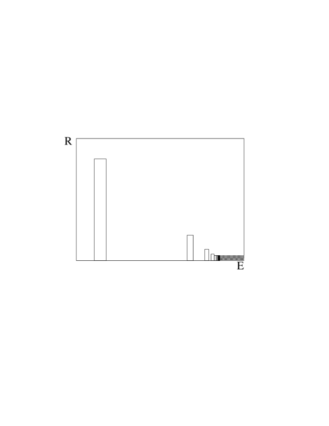
Figure 3.11: Schematic representation of resonances (wiht the area of the boxes adjusted to represent the weights of the respective delta functions) and the continuum cross section.

The explicit calculation yields

$$R(E)={9\pi\over 2\alpha^{2}}\Gamma_{e}\delta(E-E_{n})=3Q_{t}^{2}{3\over 2}\sum_{n}{k_{B}^{2}\over m^{2}}{1\over n^{3}}\pi\delta\left(E-E_{Ryd}{1\over n^{2}}\right)$$ (3.46)

for energies below threshold, and

$$R(E)=3Q^{2}_{t}{3\over 2}\beta{x\over 1-e^{-x}}$$ (3.47)

with $x=k_{B}/k=\pi\alpha/\beta$ for energies above threshold.

The perturbative expansion breaks down in the limit $\beta\to 0$. The first term of this formal series

$$\beta{x\over 1-e^{-x}}=\beta\left({x\over 2}-\ldots\right)$$ (3.48)

underestimates the exact result by a factor two.

Eq. (3.46) allows to connect the formalism based on narrow individual resonances with a formulation which is tailored to the situation at hand, namely wide overlapping resonances which merge into a smooth continuum.

Instead of summing the contributions from a large number of high radial excitations one may directly calculate the imaginary part of the Greens function for complex energy

$$\sigma(e^{+}e^{-}\to t\bar{t})=\frac{24\pi^{2}\alpha^{2}}{s}\frac{\rho_{v}(s)}{m^{2}_{t}}\left(1-\frac{16}{3}\frac{\alpha_{s}}{\pi}\right)\sum_{n}\left|\psi_{n}(0)\right|^{2}\frac{\Gamma_{t}}{(E_{n}-E)^{2}+\Gamma^{2}_{t}}$$

$$=\frac{24\pi^{2}\alpha^{2}}{s}\frac{\rho_{v}(s)}{m^{2}_{t}}\left(1-\frac{16}{3}\frac{\alpha_{s}}{\pi}\right)\sum_{n}Im\frac{\psi^{\*}_{n}(0)\psi^{*}_{n}(0)}{E_{n}-E-i\Gamma_{t}}$$

$$=-\frac{24\pi^{2}\alpha^{2}}{s}\frac{\rho_{v}(s)}{m^{2}_{t}}\left(1-\frac{16}{3}\frac{\alpha_{s}}{\pi}\right)ImG(0,0,E+i\Gamma)$$ (3.49)

The factor $\rho_{v}(s)$ incorporates the contributions from the intermediate photon and $Z$ and is given by

$$\rho^{Born}_{v}(s)=\left|e_{t}e_{e}+\frac{1}{y^{2}}\frac{\upsilon_{t}\upsilon_{e}M^{2}_{\theta}}{s-M^{2}_{Z}+iM_{Z}\Gamma_{Z}}\right|^{2}+\left|\frac{1}{y^{2}}\frac{\upsilon_{t}a_{e}M^{2}_{G}}{s-M^{2}_{Z}+iM_{Z}\Gamma_{Z}}\right|$$ (3.50)

$$\upsilon_{f}=2I_{3f}-4e_{f}\qquad a_{f}=2I_{3f}\qquad y=16\sin^{2}\theta_{W}\cos^{2}\theta_{W}$$

($\alpha=\alpha_{\rm eff}=1/128$ has been adopted in the numerical evaluation. Radiative corrections to this formula have been discussed in [92].)

The problem can be solved in closed analytical form for an exact Coulomb potential [105]

$${\rm Im}G_{E+i\Gamma_{t}}(0,0) = -{m_{t}^{2}\over 4\pi}\left[{k_{2}\over m_{t}}+{2k_{B}\over m_{t}}\arctan{k_{2}\over k_{1}}\right.$$

$$\left.+\sum_{n=1}^{\infty}{2k_{B}^{2}\over m_{t}^{2}\pi^{4}}{\Gamma_{t}k_{B}n+k_{2}\left(n^{2}\sqrt{E^{2}+\Gamma_{t}^{2}}+{k_{B}^{2}\over m_{t}}\right)\over\left(E+{k_{B}^{2}\over m_{t}n^{2}}\right)^{2}+\Gamma_{t}^{2}}\right]$$

$$k_{1,2} = \left[m_{t}\left(\sqrt{E^{2}+\Gamma_{t}^{2}}\mp E\right)/2\right]^{1/2},$$

$$k_{B} = {2\over 3}\alpha_{s}m_{t}.$$ (3.51)

To arrive at a realistic prediction of the total (and, in sect 3.2.3 of the differential) cross section the Coulomb potential must be replaced by the realistic QCD potential.

3.2.2 The QCD potential

On the basis of earlier conceptual work in [106, 107] the asymptotic behaviour of the static potential has been derived in [108, 109]. In momentum space the potential reads in the $\overline{MS}$ subtraction scheme

$$V\left(Q^{2},\alpha_{\overline{MS}}(Q^{2})\right)=-\frac{16\pi}{3}\frac{\alpha_{\overline{MS}}(Q^{2})}{Q^{2}}\left[1+\left(\frac{31}{3}-\frac{10}{9}n_{f}\right)\frac{\alpha_{\overline{MS}}(Q^{2})}{4\pi}\right]$$ (3.52)

The renormalization scale $\mu^{2}$ has been chosen as $Q^{2}$, and $n_{f}$ refers to the number of massless quarks. Employing standard arguments based on the renormalization group, the $Q^{2}$ expansion of $\alpha_{\overline{MS}}(Q^{2})$ is given by

$$\frac{\alpha_{\overline{MS}}(Q^{2})}{4\pi} = \frac{1}{b_{0}\log\left(Q^{2}/\Lambda^{2}_{\overline{MS}}\right)}\left[1-\frac{b_{1}}{b^{2}_{0}}\frac{\log\log\left(Q^{2}/\Lambda^{2}_{\overline{MS}}\right)}{\log\left(Q^{2}/\Lambda^{2}_{\overline{MS}}\right)}\right]\quad$$ (3.53)

$$b_{0} = 11-\frac{2}{3}n_{f},\qquad b_{1}=102-\frac{38}{3}n_{f}$$

The leading behaviour of the potential at small distances $[\gamma_{E}=0.5772\cdots]$

$$V(r) = \frac{16\pi}{(33-2n_{f})r\log 1/(\Lambda_{\overline{MS}}r)^{2}}$$ (3.54)

$$\left[1-\frac{b_{1}}{b^{2}_{0}}\frac{\log\log 1/(\Lambda_{\overline{MS}}r)^{2}}{\log 1/(\Lambda_{\overline{MS}}r)^{2}}+\frac{\left(\frac{31}{3}-\frac{10}{9}n_{f}\right)/b_{0}+2\gamma_{E}}{\log 1/(\Lambda_{\overline{MS}}r)^{2}}+\cdots\right]$$

is thus directly given in terms of the QCD scale parameter $\Lambda$. The exploration of $V(r)$ for small distances could thus lead to a direct determination of $\Lambda$. For quark masses above 50-100 GeV the ground state properties become independent of the potential in the nonperturbative region. As discussed in the previous section the large decay rate acts as a cutoff and the predictions are fairly insensitive to the actual regularisation. However, an additional constant which can be traded against a shift in $m_{t}$ must be carefully calibrated.

In practice one connects the theoretically predicted short distance part smoothly with the empirically determined potential above $\sim$0.1 fermi. The asymptotic form given in (3.52) is based on the assumption that $n_{f}$ species of light quarks, taken as massless, contribute to the vacuum polarization, and heavier ones are ignored. The value of $\Lambda_{\overline{MS}}$ in (3.53) must be properly related to $\Lambda_{\overline{MS}}$ as determined from other experiments with a different number of effective light flavors [110, 111]. For the momentum range of around 15 GeV explored by the $t\bar{t}$ system $n_{f}=$5 seems adequate.

In the subsequent discussion the Green’s function will be calculated in momentum space with the help of the Lippman-Schwinger integral equation [112]. The representation of the QCD potential in momentum space with the large $Q^{2}$ behaviour given by eqs. 3.52 and 3.53 will be employed. The intermediate and small momentum dependence will be based on Richardson’s potential. This choice allows to vary $\alpha_{\overline{MS}}(M_{Z}^{2})$ (or equivalently $\Lambda_{\overline{MS}}$) between 0.11 and 0.13, while maintaining a smooth $Q^{2}$ dependence of $\alpha_{V}(Q^{2})$ (Fig. 3.12).

Figure 3.12: $\alpha_{\rm eff}$ for different values of $\alpha_{s}(M_{Z})$: solid: 0.12, dashed: 0.11, dashed-dotted: 0.13, dotted: 0.10 and 0.14.

An additive constant in coordinate space (corresponding to a $\delta$-function in momentum space) is adjusted to fix $V(r=1GeV^{-1})=-1/4$ GeV for arbitrary $\alpha_{\overline{MS}}$. This constraint avoids the unmotivated and uncontroled variation of the long distance part of $V(r)$ with a change in $\alpha_{\overline{MS}}$. The potential in coordinate space is shown in Fig. 3.13.

Figure 3.13: QCD potential in the position space $V_{JKT}$ for different values of $\alpha_{s}(M_{Z})$: solid: 0.12, dashed: 0.11, dashed-dotted: 0.13, dotted: 0.10 and 0.14.

3.2.3 Realistic predictions for $\sigma_{t\bar{t}}$.

For a realistic QCD potential the Green’s function can only be calculated with numerical methods. An elegant algorithm for a solution in coordinate space has been suggested in [113]. As a consequence of the optical theorem (see also eqn. (3.49)) only the imaginary part of $G(\vec{r}=0,\vec{r}^{\prime}=0,E+i\Gamma_{t})$ is needed to predict the total cross section. The differential equation for the Green’s function

$$\left[\left(E+i\Gamma_{t}\right)-\left(-{\nabla^{2}\over m_{t}}+V(\vec{r})\right)\right]G(\vec{r},\vec{r}^{\prime}=0,E+i\Gamma_{t})=\delta(\vec{r})$$ (3.55)

is solved in a way which provides direct access to Im$G(\vec{r}=0,\vec{r}^{\prime}=0,E+i\Gamma_{t})$ without the need to calculate the full $\vec{r}$ dependence. Alternatively, in [112, 114] the Green’s function in momentum space was obtained from the Lippmann-Schwinger equation

$$G(\vec{p},E+i\Gamma_{t}) = G_{0}(\vec{p},E+i\Gamma_{t})+G_{0}(\vec{p},E+i\Gamma_{t})$$

$$\times\int{d\vec{q}\over(2\pi)^{3}}\widetilde{V}(\vec{p}-\vec{q})G(\vec{q},E+i\Gamma_{t})$$

$$G_{0}(\vec{p},E+i\Gamma_{t}) = {1\over E-p^{2}/m_{t}+i\Gamma_{t}}$$ (3.56)

The total cross section is in this case obtained from the integral over the differential distribution

$${d\sigma\over d^{3}p}={3\alpha^{2}\over\pi sm_{t}^{2}}\rho_{v}(s)\Gamma_{t}|G(\vec{p},E+i\Gamma_{t})|^{2}$$ (3.57)

This second formulation is particularly suited to introducing a momentum and energy dependent width $\Gamma(p,E)$ which allows to incorporate the phase space suppression and certain $\alpha_{s}^{2}$ rescattering corrections to be discussed below in section 3.2.6.

It is well known that the coupling of the virtual photon to the quarkonium boundstate is modified by “hard” gluon exchange. The vertex correction to the vector current produces an additional factor $\left(1-{16\over 3}{\alpha_{s}\over\pi}\right)$ for the quarkonium decay rate into $e^{+}e^{-}$ through the virtual photon or $Z$. This factor can be calculated by separating the gluon exchange [115] correction to the vertex into the instanteneous potential piece and a remainder which is attributed to gluons with high virtualities of order $m_{t}$. A similar approach has been developed in [90] for Higgs exchange. The vertex correction is again decomposed into a part which is given by the instantaneous Yukawa potential

$$V_{Yuk}(r)=-\kappa{e^{-m_{H}r}\over r}$$ (3.58)

with $\kappa=\sqrt{2}Gm_{t}^{2}/4\pi$ and a remainder which is dominated by highly virtual Higgs exchange. The rapid increase of the correction in the threshold region (cf. sect. 3.1.2) is driven by the potential; the remainder, the hard vertex correction, is fairly energy independent. The total cross section is thus sensitive to the top mass, the width (which in the SM is uniquely determined by $m_{t}$), the strong coupling constant $\alpha_{s}$ and the mass of the Higgs boson. This dependence is illustrated in Figs. 3.14-3.17. Apart from the trivial shift of the threshold due to a change in $m_{t}$ the shape of $\sigma$ is affected by the rapidly increasing width of the top quark which amounts to 0.81 GeV, 1.57 GeV and 2.24 GeV for $m_{t}=$ 150 GeV, 180 GeV, and 200 GeV respectively. This is demonstrated in Fig. 3.14: A fairly

Figure 3.14: Total cross section as function of $E=\sqrt{s}-2m_{t}$ for three values of the top quark mass.

Figure 3.15: Total cross section as function of $E=\sqrt{s}-2m_{t}$ for three values of $\alpha_{s}$.

Figure 3.16: Comparison between the predicted cross section for constant (dashed and dotted lines) and running (solid lines) $\alpha_{s}$.

Figure 3.17: Total cross section as function of $E=\sqrt{s}-2m_{t}$ for different values of the Higgs mass.

pronounced 1S peak is still visible for $m_{t}$ = 150 GeV, for $m_{t}=200$ GeV, however, only a smooth shoulder is predicted. The behaviour is qualitatively very similar, if we keep $m_{t}$ fixed say at 180 GeV and decrease or increase $\Gamma_{t}$ be the corresponding amount. The shape of the cross section will therefore allow to determine the width of the top quark. A qualitatively very different response is observed towards a change in $\alpha_{s}$ (Fig. 3.15). The binding energy increases with $\alpha_{s}$, the aparent threshold is thus lowered (This is the reason for the strong correlation between $\alpha_{s}$ and $m_{t}$ in the experimental analysis based on $\sigma_{tot}$ only [35, 116].) and the height of the “would-be resonance” is increased. Even several GeV above threshold one observes a slight increase of the cross section with $\alpha_{s}$, a consequence of the enhanced attraction between $t$ and $\bar{t}$ (cf. eq. 3.47). The impact of the running of $\alpha_{s}$ on the shape of the cross section is evident from Fig. 3.15. The full QCD prediction with running $\alpha_{s}$ (for $\alpha_{\overline{MS}}(M_{Z}^{2})$ = 0.125) is compared to the prediction for a Coulomb potential with $\alpha_{s}$ fixed. It is impossible to describe the height of the peak and the continuum above with the same value of $\alpha_{s}$, even allowing for an arbitrary additive constant $V_{0}$. The influence of a variation in $m_{H}$ is shown in Fig. 3.17. Cross section measurements with a precision better than 10% will become sensitive to the effect of a light Higgs boson.

Up to this point the amplitude induced by virtual $Z$ and $\gamma$ are included in Born approximation only. Electroweak corrections and initial state radiation are neglected. A detailed discussion of electroweak corrections to the cross section and the left right asymmetry in the context of the SM can be found in [92]. The corresponding discussion for the two-Higgs-doublet model is presented in [117]. In this model one might encounter enhanced Yukawa couplings which would amplify the effect under discussion.

Initial state radiation leads to a fairly drastic distortion of the shape of the cross section, in particular to a smearing of any pronounced structure. This is illustrated in Fig. 3.18

Figure 3.18: Comparison of the $t\bar{t}$ production cross section without (dashed) and with (solid line) initial state radiation.

where the predictions with and without initial state radiation are compared for otherwise identical parameters.

Beamstrahlung and the energy spread of the beam lead to a further smearing of the apparent cross section. These accelerator dependent issues are treated in more detail in [35]. (For a related discussion see also [116].)

3.2.4 Momentum distributions of top quarks

The Green’s function in momentum space and the momentum distribution of top quarks (and thus their decay products) are intimately related. For a narrow quarkonium resonance with orbital quantum number $n$ the quarks’ momentum distribution is evidently given by the wave function in momentum space

$${dN\over d\vec{p}}={|\widetilde{\psi}_{n}(\vec{p})|^{2}\over(2\pi)^{3}}$$ (3.59)

For $J/\psi$ or $\Upsilon$ this distribution is not directly accessible to experiment since these states decay through $Q\bar{Q}$ annihilation only. For toponium, however, which is dominated by single quark decay, the decay products carry the information of their parent momentum and hence allow for the reconstruction of the original quark momentum distribution [118].

For one individual resonance this leads to the differential $t\bar{t}$ cross section (without $Z$ contribution and transverse gluon correction).

$${d\sigma_{n}\over d\vec{p}}(\vec{p},E)={3\alpha^{2}Q_{t}^{2}\over\pi sm_{t}^{2}}|\psi_{n}(\vec{r}=0)|^{2}{\Gamma_{t}\over(E-E_{n})^{2}+\Gamma_{t}^{2}}|\widetilde{\psi}_{n}(\vec{p})|^{2}$$ (3.60)

Once $\Gamma_{t}$ is sufficiently large, interferences between different radial excitations become important and the right-hand side of this equation has to be replaced by the square of the Green’s function [119, 112]

$${d\sigma_{n}\over d\vec{p}}(\vec{p},E)={3\alpha^{2}Q_{t}^{2}\over\pi sm_{t}^{2}}\Gamma_{t}\left|G(\vec{p},E+i\Gamma_{t})\right|^{2}$$ (3.61)

with

$$G(\vec{p},E+i\Gamma_{t})=\int d\vec{r}e^{i\vec{p}\vec{r}}G(\vec{r},\vec{r}^{\prime}=0,E+i\Gamma_{t})$$ (3.62)

As discussed in sect. 3.2.2, the Green’s function can be obtained in momentum space as a solution of the Lippmann-Schwinger equation. For an energy close to the 1S peak it exhibits a fairly smooth behaviour reminiscent of the 1S wave function in momentum space (Fig. 3.19).

 

Figure 3.19: Real (dashed) and imaginary (dotted) parts of the Green’s function for an energy corresponding to the 1S peak (upper figure) and for $E=0$ (lower figure). Solid curve: $|pG(p)|^{2}\cdot 0.002.$

With increasing energy an oscillatory pattern of the amplitude is observed, and a shift towards larger momenta (Fig. 3.19). These results are intentionally displayed for $m_{t}=120$ GeV, where the oscillations are still clearly visible, in contrast to $m_{t}$=180 GeV where all oscillations are smeared by the large width $\Gamma_{t}$. The corresponding predictions for the distributions at $m_{t}=180$ GeV are displayed in Fig. 3.20.

Figure 3.20: Momentum distribution of top quarks for three different cms energies.

Figure 3.21: Energy distribution of $W$’s from top quark decay for three different cms energies.

The transition from a wide distribution below the nominal threshold to a narrow one with the location of the peak determined by trivial kinematics is clearly visible. The impact on the energy distribution of the $W$’s from top decay is shown in Fig. 3.21.

To characterize the momentum distribution by a single parameter, one may either choose its peak value, or the expectation value of the modulus of the momentum $\langle p\rangle$, the latter being well adopted to the experimental analysis. In the situation at hand the definition of $\langle p\rangle$ has to be introduced with some care. The free Green’s function $G_{0}$ (see eq. 3.56) drops $\sim p^{-2}$ for large momenta and this behaviour is recovered also in the presence of interaction. The expectation value $\langle p\rangle$ diverges logarithmically with the cutoff. In the narrow width approximation one finds for the leading terms

$$\langle p\rangle = {\int_{0}^{p_{m}}d\vec{p}p\left|G_{0}(\vec{p},E+i\Gamma)\right|^{2}\over\int_{0}^{p_{m}}d\vec{p}\left|G_{0}(\vec{p},E+i\Gamma)\right|^{2}}$$ (3.63)

$$= \sqrt{m_{t}E}\left(1+{\Gamma\over E}{\ln p_{m}^{2}/\left(\sqrt{E^{2}+\Gamma^{2}}m_{t}\right)\over\pi}\right)$$

where a cutoff $p_{m}$ has been introduced. As a consequence of the small numerical prefactor of the divergent term and its logarithmic cutoff dependence the result is fairly insensitive to the exact value of the cutoff for $p_{m}$ of order $m_{t}$. Alternatively one may replace the phase space element $d\vec{p}/m_{t}$ by the relativistic version $d\vec{p}/E=d\vec{p}/\sqrt{m_{t}^{2}+p^{2}}$ to obtain a convergent result. In future measurements the cutoff will presumably be provided by the experimental analysis.

In order to study the dependence of $\langle p\rangle$ on the strong coupling constant, consider for the moment the predictions for a stable quark. Some intuition and qualitative understanding can already be gained from the predictions based on a pure Coulomb potential [120].

For a stable top quark of fixed mass the “effective threshold” can be associated with the location of the $1S$ resonance $\sqrt{s_{thr}}=2m_{t}+E_{1S}$ with $E_{1S}=-E_{Ryd}=-\alpha^{2}m_{t}/4$ which decreases with increasing $\alpha$. The height of the resonance cross section is proportional to the square of the wave function at the origin and hence proportional to $\alpha^{3}$, as long as the resonances are reasonably well separated. In the limit of large $\Gamma_{t}$, i.e. far larger than $E_{Ryd}$, the overlapping $1S$, $2S$ $\dots$ resonances have to fill the gaps between the peaks. Since these gaps themselves increase proportional to $\alpha^{2}$, one is left in the extreme case of large width with a cross section linear in $\alpha$. Note that this corresponds to the behaviour of the cross section close to but slightly above the threshold which is also proportional to $\alpha$.

For realistic top masses one thus observes a dependence of the peak cross section linear in $\alpha$. Since the location of the peak itself depends on $\alpha$, only the analysis of the full shape allows to extract the relevant information.

In a next step also the momentum distribution of top quarks has to be exploited to obtain further information. The discussion is again particularly simple for the Coulomb potential $V(r)=-\alpha/r$ and provides a nice exercise in nonrelativistic quantum mechanics. The average momentum, in units of the Bohr momentum $\alpha m_{t}/2$, can be written in terms of a function $f(\epsilon)$ which depends only on one variable $\epsilon=E/E_{Ryd}$ if the energy $E=\sqrt{s}-2m_{t}$ is measured in terms of the Rydberg energy.

$$\langle p\rangle=\frac{\alpha m_{t}}{2}f(\epsilon)$$ (3.64)

For positive arguments the function $f$ can be derived from obvious kinematical considerations.

$$f(\epsilon)=\sqrt{\epsilon}\qquad{\rm for}\qquad\epsilon\geq 0$$ (3.65)

For the discrete negative arguments $\epsilon_{n}=-1/n^{2}$, corresponding to the locations of the bound states, the radial wave functions in momentum space are given in terms of the Gegenbauer polynomials $C^{m}_{n}$

$$\psi(\vec{p}\,)=\frac{16\pi n^{3/2}}{(1+n^{2}p^{2})^{2}}C^{1}_{n-1}\left(\frac{n^{2}p^{2}-1}{n^{2}p^{2}+1}\right)Y_{0}^{0}\left(\theta,\varphi\right)$$ (3.66)

with

$$\int\frac{d\vec{p}}{(2\pi)^{3}}|\psi(\vec{p}\,)|^{2}=1\ .$$ (3.67)

Using the explicit forms of $C^{m}_{n}$

$$C^{1}_{0}(z)=1,\qquad C^{1}_{1}(z)=2z,\qquad C^{1}_{2}(z)=4z^{2}-1$$ (3.68)

one obtains through straightforward calculation

$$f(-1)=\frac{8}{3\pi},\qquad f(-1/4)=\frac{16}{15\pi},\qquad f(-1/9)=\frac{24}{35\pi}\ .$$ (3.69)

For arbitrary $n$ one derives the general result

$$f\left(-\frac{1}{n^{2}}\right)=\frac{8n}{(2n-1)(2n+1)\pi}$$ (3.70)

with the asymptotic behaviour

$$f\left(-\frac{1}{n^{2}}\right)\to\frac{2}{n\pi}\ .$$ (3.71)

This is in accord with the result expected from classical mechanics: For the average momentum of a particle on a closed orbit in the Coulomb potential one derives

$$\langle p^{2\beta}\rangle=\left(\frac{\alpha m_{t}}{2}\right)^{2\beta}\left(\frac{-E}{E_{Ryd}}\right)^{\beta}\frac{1}{2\pi}\int_{0}^{2\pi}d\xi\frac{(1-e^{2}\cos^{2}\xi)^{\beta}}{(1-e\cos\xi)^{2\beta-1}}\ .$$ (3.72)

Quantum mechanical orbits with angular momentum zero and high radial quantum numbers correspond to classical motions with excentricity $e=1$ (i.e. straight lines). In this limiting case the classical expectation value is easily evaluated, and for $\beta=1/2$ one finds agreement with the quantum mechanical result. For small negative energies one therefore obtains the behaviour $f(\epsilon)=2\sqrt{-\epsilon}/\pi$. Significantly below threshold, however, the average momentum obtained from the Green’s function increases more rapidly with decreasing energy and between the $1S$ and the $2S$ state one observes an approximately linear dependence on the energy.

From these considerations the dependence of the average momentum on $\alpha$ (with $E$ fixed) is easily understandable, in particular the seemingly surprising observation that well below threshold $\langle p\rangle$ decreases with increasing $\alpha$. From (3.64) one derives for a shift in $\alpha$ (keeping the energy $E$ fixed) the following shift in $\langle p\rangle$

$$\frac{\delta\langle p\rangle}{\langle p\rangle}=\left(1-2\frac{f^{\prime}(\epsilon)}{f(\epsilon)}\epsilon\right)\frac{\delta\alpha}{\alpha}\ .$$ (3.73)

Above threshold as well as close to but below threshold $f\propto\sqrt{|\epsilon|}$. Hence $\epsilon f^{\prime}/f=1/2$ and the average momentum remains unaffected. The location of the minimum is thus an ideal place to fix the mass of the top quark. Significantly below threshold, however, $\epsilon f^{\prime}/f\approx 1$ and the factor in front of $\delta\alpha/\alpha$ becomes negative. This explains the decrease of $\langle p\rangle$ with increasing $\alpha$.

Figure 3.22: a) Average momentum as a function of $E$ for different values of $\alpha_{s}$. The markers show the results of the analytical calculation at $1S$, $2S$, $3S$ energies. b) Comparison with the analytical result for discrete energies and with the square–root dependence close to threshold.

These results are illustrated in Fig.3.22. In Fig.3.22b we demonstrate that $\langle p\rangle$ as evaluated with the program for the Green function (solid line) coincides perfectly well with the values calculated from the analytical formula on resonance, indicated by the triangles. The prediction from classical mechanics, namely $\langle p\rangle\propto\sqrt{|\epsilon|}$ is shown by the dotted line and agrees nicely for positive and negative energies. In Fig.3.22a $\alpha_{s}$ is increased from 0.20 to 0.24 and $\langle p\rangle$ changes in accord with the previous discussion.

For definiteness we have chosen $m=m_{t}/2=60$ GeV for the reduced mass and $\alpha=4\alpha_{s}/3$ with $\alpha_{s}$ varying between 0.20 and 0.24. The curves demonstrate the decrease of $\langle p\rangle$ by about 10% for the corresponding increase in $\alpha$. The triangles mark the locations of the resonances and the expectation values for the momentum as calculated from (3.70).

Figure 3.23: Energy dependence of $\langle p\rangle$, the average t quark momentum for $\alpha_{s}=0.13$ (dotted) $0.12$ (dashed) and $0.11$ (solid) line for $m_{t}=120$ GeV. a) $\Gamma_{t}=0.03$ GeV and b) $\Gamma_{t}=0.3$ GeV.

The qualitative behaviour remains unchanged for realistic QCD potentials corresponding to different values of $\alpha_{s}(M_{Z})$. Qualitatively the same behaviour is observed as in Fig.3.22. In Fig.3.23a the top quark width has been set to an artificially small value of $0.03$ GeV, in Fig.3.23b the realistic value of $0.3$ GeV has been adopted. The finite width leads to an additional contribution to the momentum of order $\sqrt{\Gamma m}$.

An important feature is evident from Fig.3.23: The momentum calculated for positive energy is nearly independent from $\alpha_{s}$ and reflects merely the kinematic behaviour, just as in the case of the Coulomb potential. This is characteristic for the choice of a potential [114] where the large distance behaviour is fixed by phenomenology and decoupled from the short distance value of $\alpha_{s}$.

The different assumptions on the long distance behaviour are reflected in differences between the predictions of [121, 119, 112] for the precise location of the $t\bar{t}$ threshold for identical values of $\alpha_{s}$ and $m_{t}$ and in differences in the $\alpha_{s}$ dependence of the momentum distributions for fixed $m_{t}$ and energy (see also [116]). All these differences can be attributed to the freedom in the additive constant discussed before. The same additive constant appears in $b\bar{b}$ spectroscopy, such that the mass difference between top and bottom is independent from these considerations.

In Fig. 3.24 the predictions for $\langle p\rangle$ vs. energy are presented for the case of a realistic QCD potential, assuming $m_{t}=120/150/180$ GeV. The strong rise of $\langle p\rangle$ as a consequence of the strong increase of $\Gamma_{t}$ is clearly visible.

Figure 3.24: Energy dependence of the average top quark momentum for $m_{t}$ = 120/150/180 GeV. Triangles, stars and circles correspond to $\langle p_{t}\rangle$ for S-states with $\Gamma_{t}=0$.

3.2.5 Angular distributions and polarization

Close to threshold the production amplitude is dominantly $S$-wave which leads to an isotropic angular distribution. The spin of top quarks is alligned with the beam direction, with a degree of polarization determined by the electroweak couplings, the beam polarization and the mass of the top quark, but independent of the production dynamics, in particular of the potential.

Small, but nevertheless experimentally accessible corrections do arise from the small admixture of $P$-wave contributions and from rescattering of the top quark decay products. Let us concentrate for the moment on the first mechanism. $P$-wave amplitudes are proportional to the top quark momentum. For stable noninteracting particles the momentum vanishes at threshold. However, as discussed in the previous section the expectation value of the quark momentum is nonzero for all energies — a consequence of the large top decay rate and the uncertainty principle. Technically the $P$-wave contribution is calculated with the help of the Green’s function technique. The generalization of the Lippman-Schwinger equation (3.56) from $S$- to $P$-waves reads as follows

$${\cal F}({\rm p},E) = G_{0}(p,E)+G_{0}(p,E)\int{d^{3}k\over(2\pi)^{3}}{{\bf p}\cdot{\bf k}\over{\bf p}^{2}}V({\bf p}-{\bf k}){\cal F}(k,E)$$ (3.74)

It is then straightforward to calculate the differential momentum distribution and the polarization of top quarks produced in electron positron annihilation. Let us recall the following conventions for the fermion couplings

$$v_{f}=2I^{3}_{f}-4q_{f}\sin^{2}\theta_{\rm W},\qquad a_{f}=2I^{3}_{f}.$$ (3.75)

$P_{\pm}$ denotes the longitudinal electron/positron polarization and $\chi=(P_{+}-P_{-})/(1-P_{+}P_{-})$ can be interpreted as effective longitudinal polarization of the virtual intermediate photon or $Z$ boson. The following abbreviations will be useful below:

$$a_{1} = q_{e}^{2}q_{t}^{2}+(v_{e}^{2}+a_{e}^{2})v_{t}^{2}d^{2}+2q_{e}q_{t}v_{e}v_{t}d$$

$$a_{2} = 2v_{e}a_{e}v_{t}^{2}d^{2}+2q_{e}q_{t}a_{e}v_{t}d$$

$$a_{3} = 4v_{e}a_{e}v_{t}a_{t}d^{2}+2q_{e}q_{t}a_{e}a_{t}d$$ (3.76)

$$a_{4} = 2(v_{e}^{2}+a_{e}^{2})v_{t}a_{t}d^{2}+2q_{e}q_{t}v_{e}a_{t}d$$

$$d = {1\over 16\sin^{2}\theta_{\rm W}\cos^{2}\theta_{\rm W}}\,{s\over s-M_{Z}^{2}}.$$

The differential cross section, summed over polarizations of quarks and including $S$-wave and $S$-$P$–interference contributions, is thus given by

$${d^{3}\sigma\over dp^{3}} = {3\alpha^{2}\Gamma_{t}\over 4\pi m_{t}^{4}}(1-P_{+}P_{-})\left[{(a_{1}+\chi a_{2})\left(1-{16\alpha_{\rm s}\over 3\pi}\right)\left|G({\rm p},E)\right|^{2}+}\right.$$ (3.77)

$$\left.{+(a_{3}+\chi a_{4})\left(1-{12\alpha_{\rm s}\over 3\pi}\right){{\rm p}\over m_{t}}{\rm Re}\left(\,G({\rm p},E)F^{*}({\rm p},E)\,\right)\,\cos\vartheta}\right].$$

The vertex corrections from hard gluon exchange for $S$-wave and $P$-wave amplitudes are included in this formula. It leads to the following forward-backward asymmetry [122, 123]

$${\cal A}_{\rm FB}({\rm p},E)=C_{\rm FB}(\chi)\,\varphi_{\rm{}_{R}}({\rm p},E),$$ (3.78)

with

$$C_{\rm FB}(\chi)={1\over 2}\,{a_{3}+\chi a_{4}\over a_{1}+\chi a_{2}},$$ (3.79)

$\varphi_{\rm{}_{R}}={\rm Re}\,\varphi$, and

$$\varphi({\rm p},E)={(1-{4\alpha_{\rm s}/3\pi})\over(1-{8\alpha_{\rm s}/3\pi})}\,{{\rm p}\over m_{t}}\,{F^{*}\!({\rm p},E)\over G^{*}\!({\rm p},E)}.$$ (3.80)

This result is still differential in the top quark momentum. Replacing $\varphi({\rm p},E)$ by

$$\Phi(E)={(1-{4\alpha_{\rm s}/3\pi})\over(1-{8\alpha_{\rm s}/3\pi})}\,{\int_{0}^{{\rm p}_{m}}d{\rm p}\,{{\rm p}^{3}\over m_{t}}\,F^{*}({\rm p},E)G({\rm p},E)\over\int_{0}^{{\rm p}_{m}}d{\rm p}\,{\rm p}^{2}\left|G({\rm p},E)\right|^{2}}.$$ (3.81)

one obtains the integrated forward-backward asymmetry again. Again, the cutoff ${\rm p}_{m}$ must be introduced to eliminate the logarithmic divergence of the integral.

Figure 3.25: Definition of the spin directions. The normal component ${\bf s}_{\rm N}$ points out of the plane.

Polarization [123, 127]
To describe top quark polarization in the threshold region it is convenient to align the reference system with the beam direction (Fig. 3.25) and to define

$${\bf s}_{\|}={\bf n}_{e^{-}},\quad{\bf s}_{\rm N}={{\bf n}_{e^{-}}\times{\bf n}_{t}\over|{\bf n}_{e^{-}}\times{\bf n}_{t}|},\quad{\bf s}_{\bot}={\bf s}_{\rm N}\times{\bf s}_{\|}.$$ (3.82)

In the limit of small $\beta$ the quark spin is essentially aligned with the beam direction apart from small corrections proportional to $\beta$, which depend on the production angle. A system of reference with ${\bf s}_{\|}$ defined with respect to the top quark momentum [124] is convenient in the high energy limit but evidently becomes less convenient close to threshold.

Including the QCD potential one obtains for the three components of the polarization

$${\cal P}_{\|}({\bf p},E,\chi) = C_{\|}^{0}(\chi)+C_{\|}^{1}(\chi)\,\varphi_{\rm{}_{R}}({\rm p},E)\,\cos\vartheta\,$$ (3.83)

$${\cal P}_{\bot}({\bf p},E,\chi) = C_{\bot}(\chi)\,\varphi_{\rm{}_{R}}({\rm p},E)\,\sin\vartheta\,$$ (3.84)

$${\cal P}_{\rm N}({\bf p},E,\chi) = C_{\rm N}(\chi)\varphi_{\rm{}_{I}}({\rm p},E)\sin\vartheta\,,$$ (3.85)

$$\hskip 21.52771ptC_{\|}^{0}(\chi)=-{a_{2}+\chi a_{1}\over a_{1}+\chi a_{2}},\hskip 29.7082ptC_{\|}^{1}(\chi)=\left(1-\chi^{2}\right){a_{2}a_{3}-a_{1}a_{4}\over\left(a_{1}+\chi a_{2}\right)^{2}},$$

$$\hskip 21.52771ptC_{\bot}(\chi)=-{1\over 2}\,{a_{4}+\chi a_{3}\over a_{1}+\chi a_{2}},\qquad C_{\rm N}(\chi)=-{1\over 2}\,{a_{3}+\chi a_{4}\over a_{1}+\chi a_{2}}\,=\,-C_{\rm FB}(\chi),$$

with $\varphi_{\rm{}_{I}}={\rm Im}\,\varphi$, and $\varphi({\rm p},E)$ as defined in (3.80). The momentum integrated quantities are obtained by the replacement $\varphi({\rm p},E)\to\Phi(E)$. The case of non-interacting stable quarks is recovered by the replacement $\Phi\to\beta$, an obvious consequence of (3.81).

Let us emphasize the main qualitative features of the result:

• Top quarks in the threshold region are highly polarized. Even for unpolarized beams the longitudinal polarization amounts to about $-0.41$ and reaches $\pm 1$ for fully polarized electron beams. This later feature is of purely kinematical origin and independent of the structure of top quark couplings. Precision studies of polarized top decays are therefore feasible.

• Corrections to this idealized picture arise from the small admixture of $P$-waves. The transverse and the normal components of the polarization are of order 10%. The angular dependent part of the parallel polarization is even more suppressed. Moreover, as a consequence of the angular dependence its contribution vanishes upon angular integration.

• The QCD dynamics is solely contained in the functions $\varphi$ or $\Phi$ which is the same for the angular distribution and the various components of the polarization. (However, this “universality” is affected by the rescattering corrections.) These functions which evidently depend on QCD dynamics can thus be studied in a variety of ways.

• The relative importance of $P$-waves increases with energy, $\Phi\sim\sqrt{E/m_{t}}$. This is expected from the close analogy between $\Phi_{\rm R}={\rm Re}\,\Phi$ and $\beta$. In fact, the order of magnitude of the various components of the polarization above, but close to threshold, can be estimated by replacing $\Phi_{\rm R}\to{\rm p}/m_{t}$.

The $C_{i}$ are displayed in Fig. 3.26 as functions of the variable $\chi$ ($\sin^{2}\!\theta_{\rm W}=0.2317$, $m_{t}=180$ GeV). As discussed before, $C_{\|}^{0}$ assumes its maximal value $\pm 1$ for $\chi=\mp 1$ and the coefficient $C_{\|}^{1}$ is small throughout. The coefficient $C_{\bot}$ varies between $+0.7$ and $-0.5$ whereas $C_{\rm N}$ is typically around $-0.5$. The dynamical factors $\Phi$ are around $0.1$ or larger, such that the $P$-wave induced effects should be observable experimentally.

Figure 3.26: The coefficients (LABEL:coefs) for $\sqrt{s}/2=m_{t}=180$ GeV.

The normal component of the polarization which is proportional to $\varphi_{\rm{}_{I}}$ has been predicted for stable quarks in the framework of perturbative QCD [125, 124]. In the threshold region the phase can be traced to the $t\bar{t}$ rescattering by the QCD potential. For stable quarks, assuming a pure Coulomb potential $V=-4\alpha_{\rm s}/3r$, the nonrelativistic problem can be solved analytically [126] and one finds

$$\lim_{\Gamma_{t}\rightarrow 0\atop E\rightarrow{\bf p}^{2}/m_{t}}\left(E-{{\bf p}^{2}\over m_{t}}+i\Gamma_{t}\right)G({\rm p},E) = \exp\left(\pi{\bar{k}}\over 2{\rm p}\right)\,\Gamma(1+{i{\bar{k}}/{\rm p}})$$ (3.87)

$$\lim_{\Gamma_{t}\rightarrow 0\atop E\rightarrow{\bf p}^{2}/m_{t}}\left(E-{{\bf p}^{2}\over m_{t}}+i\Gamma_{t}\right)F({\rm p},E) = \left(1-i{{\bar{k}}\over{\rm p}}\right)\exp\left(\pi{\bar{k}}\over 2{\rm p}\right)\,\Gamma(1+{i{\bar{k}}/{\rm p}}),\ \ \ \ \$$ (3.88)

with ${\bar{k}}=2m_{t}\alpha_{s}/3$ and hence

$$\varphi_{\rm{}_{I}}({\rm p},E) \rightarrow {2\over 3}\alpha_{\rm s}{1-4\alpha_{\rm s}/3\pi\over 1-8\alpha_{\rm s}/3\pi}$$ (3.89)

$$\Phi_{\rm I}(E) \rightarrow {2\over 3}\alpha_{\rm s}{1-4\alpha_{\rm s}/3\pi\over 1-8\alpha_{\rm s}/3\pi}.$$ (3.90)

The component of the polarization normal to the production plane is thus approximately independent of $E$ and essentially measures the strong coupling constant. In fact one can argue that this is a unique way to get a handle on the scattering of heavy quarks through the QCD potential.

Predictions for real and imaginary parts of the function $\varphi$ are displayed in Fig. 3.27 for four different energies.

Figure 3.27: Real (solid) and imaginary (dashed) part of the function $\varphi({\rm p},E)$ for $m_{t}=180$ GeV, $\alpha_{\rm s}=0.125$ and four different energies. The dotted line shows the free particle case ${\rm Re}\,\varphi=\mbox{p}/m_{t}$ (from [127]).

The momentum integrated functions $\Phi(E)$ are shown in Fig. 3.28. From this figure, in combination with Fig. 3.26, it is clear that the contribution of $P$-wave amplitudes to the quark polarization will amount to 10% at most and by construction vanishes upon angular integration.

Figure 3.28: Real and imaginary part of $\Phi(E)$ for three different values of $\alpha_{\rm s}$ (from [127]).

3.2.6 Rescattering

For a particle with a very small decay rate production and decay amplitudes can be clearly separated. This is fairly evident from the space-time picture of such a sequence. Prior to its decay the particle travels away from the production point and any coherence is lost between the two reactions. The situation is different for the case under discussion, an unstable top quark which decays within the range of interaction between $t$ and $\bar{t}$. In such a situation the decay products from $t$ are still affected by the force originating from $\bar{t}$ and vice versa (Fig. 3.29).

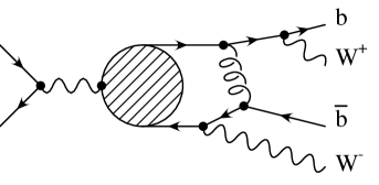
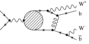
a)	b)

Figure 3.29: Lowest order rescattering diagrams.

In ref. [128, 129] it has been demonstrated that the total cross section remains unaffected by rescattering in order $\alpha_{s}$. This result had been anticipated in [112] on the basis of earlier work which considered the decay rate of a muon bound in the strong field of a nucleus [130]. In contrast momentum and angular distributions [122, 129, 131] as well as the top quark polarization [127] are affected by rescattering. For example the momentum distribution has to be corrected by a factor $(1+\psi_{1}(p,E))$ with

$$\psi_{1}({\rm p},E)=2\,{\rm Im}\int\!\frac{d^{3}k}{(2\pi)^{3}}V(|{\bf k}-{\bf p}|)\frac{G({\rm k},E)}{G({\rm p},E)}\frac{\arctan{\frac{|{\bf k}-{\bf p}|}{\Gamma_{t}}}}{|{\bf k}-{\bf p}|}$$ (3.91)

a) E=-3GeV	b) E=0GeV
c) E=2GeV	d) E=5GeV

Figure 3.30: Modification of the momentum distribution through rescattering. Dashed line: no rescattering corrections included; Solid line: rescattering contribution with full potential included; dotted line: rescattering contribution with pure Coulomb potential and $\alpha_{\rm s}=0.187$ included (from [127]).

The distribution is shifted towards smaller momenta by about 5% (Fig. 3.30), an effect that could become relevant in precision experiments. The influence on the forward-backward asymmetry and the polarization is even more pronounced [127], as far as the $S$-$P$-wave interference terms are concerned which are thus intrinsically of order $\beta$. A detailed discussion of these effects is beyond the scope of these lectures and can be found in [127].

3.2.7 Relativistic corrections

In ${\cal O}(\alpha^{2}_{s})$ one anticipates effects from relativistic corrections, from the reduction of the phase space through the binding energy and from the Coulomb wave function of the $b$ quark. Individually these effects are large. For the sake of the argument, let us adopt a pure Coulomb potential and a binding energy of -2.5 GeV. From the virial theorem one derives a potential energy of -5 GeV. The phase space of the quark decaying first is therefore reduced by this same amount. Assuming $m_{t}=180$ GeV one would arrive at a reduction of $\Gamma_{t}$ by about 10%. A full calculation of all ${\cal O}(\alpha^{2}_{s})$ effects is not available at present and one has to resort to models and analogies [112, 119, 114]. For example, it has been shown [130, 132] that the decay rate of a muon bound in the field of a nucleus is given by

$$\Gamma=\Gamma_{\rm free}\left[1-5(Z\alpha)^{2}\right]\left[1+5(Z\alpha)^{2}\right]\left[1-{(Z\alpha)^{2}\over 2}\right],$$ (3.93)

where the first correction factor originates from the phase space suppression, the second from the Coulomb enhancement, and the third from time dilatation. Thus there is no first order correction to the total rate from rescattering in the nucleus potential, similar to the $t\bar{t}$ case discussed above. The second order contributions evidently compensate to a large extent. In a model calculation where these features are implemented [114] through a momentum dependent width, it is found that the total cross section as well as the momentum distribution are hardly affected. These considerations have recently been confirmed in a more formal approach [133].

Acknowledgments

I would like to thank A. Czarnecki, R. Harlander, A. Hoang, M. Jeżabek, E. Mirkes, M. Peter, T. Teubner, and P. Zerwas for pleasant collaborations and many helpful discussions and comments on the TOPics presented in this review. I am particularly grateful to A. Czarnecki. Without his TeXnical help this paper would never have been completed. The hospitality of the SLAC theory group during my sabbatical in the summer term 1995 is gratefully acknowledged.

Bibliography

-
[1]
P. Sinerva, these proceedings;
CDF Collaboration (F. Abe et al.), Phys. Rev. Lett. 74 (1995) 2626;
D0 Collaboration (S. Abachi et al.), Phys. Rev. Lett. 74 (1995) 2632. - [2] D. Bardin et al., in Reports of the Working Group on Precision Calculations for the -Resonance, CERN 95-03, pg. 7.
- [3] W. Hollik, talk at Int. Europhysics Conf. on HEP, Brussels, 1995, KA-TP-15-1995, hep-ph/9512232.
- [4] M. Swartz , these proceedings, and references therein.
- [5] For a recent compilation of theoretical results see B. Kniehl, in Reports of the Working Group on Precision Calculations for the -Resonance, CERN 95-03, pg. 299.
- [6] A. Sirlin, ibid. pg. 299.
- [7] G. Degrassi et al., ibid. pg. 163.
- [8] W.A. Bardeen, C.T. Hill, M. Lindner, Phys. Rev. D 41 (1990) 1647.
- [9] G.L. Kane and M.E. Peskin, Nucl. Phys. B 195 (1982) 29.
- [10] C. Albajar et al. [UA1 Coll.], Phys. Lett. B256 (1991) 121, E: ibid. B262 (1991) 497.
- [11] Particle Data Group, Phys. Rev. D50, 1171 (1994).
- [12] A. Djouadi, J.H. Kühn and P.M. Zerwas, Z. Phys. C 46 (1990) 411.
- [13] Dong Su, private communication.
-
[14]
TOPAZ Coll., E. Nakano et al., Phys. Lett. B340 (1994) 135.
AMY Coll., F. Liu et al., Phys. Rev. D49 (1994) 4339.
For a recent review see e.g. K. Miyabayashi, in Recent electroweak results from TRISTAN in XXXth Rencontres de Moriond. - [15] D. Schaile and P.M. Zerwas, Phys. Rev. D45 (1992) 3262.
- [16] M. Chanowitz, M. Furman and I. Hinchliffe, Nucl. Phys. B 153 (1979) 402.
- [17] N. Cabibbo, L. Maiani, G. Parisi and R. Petronzio, Nucl. Phys. B 158 (1979) 296.
- [18] M. Lindner, Z. Phys. C 31 (1986) 295.
- [19] G. Münster, Nucl. Phys. B (Proc. Suppl.) 34 (1994) 596; ibid., 42 (1995) 162.
- [20] L. Hall, these proceedings.
- [21] H. Albrecht et al. (ARGUS), Phys. Lett. B 192 (1987) 245. M. Artuso et al. (CLEO), Phys. Rev. Lett. 62 (1989) 2233.
- [22] M. Veltman, Act. Phys. Pol. B 8 (1977) 475.
- [23] M. Veltman, Nucl. Phys. B 123 (1977) 89.
- [24] L. Avdeev et al., Phys. Lett. B 336 (1994) 560; Erratum ibid. B349 (1995) 597.
- [25] K.G. Chetyrkin, J.H. Kühn, and M. Steinhauser, Phys. Lett. B 351 (1995) 331, Phys. Rev. Lett. 75 (1995) 3394.
-
[26]
J.H. Kühn, Act. Phys. Pol. B 12 (1981) 347.
J.H. Kühn, Act. Phys. Austr. Suppl.XXIV (1982) 203. - [27] M. Jeżabek and J. H. Kühn, Phys. Lett. B 207 (1988) 91.
- [28] B. H. Smith and M. B. Voloshin, Phys. Lett. B 340 (1994) 176.
- [29] A. Czarnecki, Act. Phys. Pol. B 26 (1995) 845.
- [30] S. J. Brodsky, G. P. Lepage, and P. B. Mackenzie, Phys. Rev. D 28 (1983) 228.
- [31] A. Denner and T. Sack, Nucl. Phys. B 358 (1991) 46.
- [32] R. Migneron G. Eilam, R.R. Mendel and A. Soni, Phys. Rev. Lett. 66 (1991) 3105.
- [33] A. Denner and A.H. Hoang, Nucl. Phys. B397 (1993) 483.
- [34] M. Jeżabek and J. H. Kühn, Phys. Rev. D 48 (1993) R1910; E: ibid. D49 (1994) 4970.
- [35] K. Fujii, these proceedings.
- [36] J.H. Kühn and K.H. Streng, Nucl. Phys. B 198 (1982) 71.
- [37] M. Jeżabek and J. H. Kühn, Nucl. Phys. B 320 (1989) 20.
-
[38]
A. Czarnecki, M. Jeżabek, and J. H. Kühn, Act. Phys. Pol. B 20 (1989) 961,
E: ibid, B23 (1992) 173.
M. Jeżabek and C. Jünger, Act. Phys. Pol. B 24 (1993) 1923. - [39] A. Czarnecki, M. Jeżabek, and J. H. Kühn, Nucl. Phys. B 351 (1991) 70.
- [40] A. Czarnecki, M. Jeżabek, J. G. Körner, and J. H. Kühn, Phys. Rev. Lett. 73 (1994) 384.
- [41] A. Czarnecki and M. Jeżabek, Nucl. Phys. B 427 (1994) 3.
-
[42]
G.L. Kane, Proceedings, Madison Workshop 1979;
I. Bigi et al. in Ref.[43];
J.F. Gunion, H.E. Haber, G. Kane and S. Dawson, The Higgs Hunter’s Guide, Addison–Wesley 1990;
C.S. Li and T.C. Yuan, Phys. Rev. Lett. 42 (1990) 3088. - [43] I. Bigi, Y.L. Dokshitzer, V.A. Khoze, J. Kühn and P. Zerwas, Phys. Lett. B 181 (1986) 157.
- [44] E. Reya, P.M. Zerwas [conv.] et al., in Proceedings ECFA LHC Workshop, Aachen 1990, CERN 90–10.
- [45] P. Igo-Kemenes, J.H. Kühn [conv.], Proceedings, Collisions at 500 GeV: The Physics Potential, DESY 92-123, pg. 255-326, pg. 327-378.
-
[46]
A. Czarnecki and S. Davidson,
Phys. Rev. D48 (1993) 4183; ibid., D47 (1993) 3063.
A. Czarnecki and A.I. Davydychev, Phys. Lett. B 325 (1994) 435. - [47] A. Czarnecki, Phys. Rev. D 48 (1993) 5250.
-
[48]
J. Gunion et al., Ref.[42];
A. Mendez and A. Pomarol, Phys. Lett. B 252 (1990) 461;
C.S. Li and R.J. Oakes, Phys. Rev. D 43 (1991) 855. -
[49]
K. Hikasa and M. Kobayashi, Phys. Rev. D 36 (1987) 724;
H. Baer, M. Drees, R. Godbole, J.F. Gunion and X. Tata, Tallahassee Report FSU–HEP–910308 (1991). - [50] K. Hidaka, Y. Kizukuri and T. Kon, Gakugei Report TGU–12 (1991).
-
[51]
J. Ellis and S. Rudaz, Phys. Lett. B 128 (1983) 248;
A. Bouquet, J. Kaplan and C. Savoy, Nucl. Phys. B 262 (1985) 299. - [52] G. Eilam, J.L. Hewett and A. Soni, Phys. Rev. D 44 (1991) 1473;
- [53] H. Fritzsch, Phys. Lett. B 224 (1989) 423.
- [54] W. Buchmüller and M. Gronau, Phys. Lett. B 220 (1989) 641.
-
[55]
M. Glück, J.F. Owens and E. Reya,
Phys. Rev. D 15 (1978) 2324;
B.L. Combridge, Nucl. Phys. B 151 (1979) 429. -
[56]
S. Willenbrock and D.A. Dicus, Phys. Rev. D 34 (1986) 155;
C.–P. Yuan, Phys. Rev. D 41 (1990) 42. - [57] A.D. Martin, W.J. Stirling, and R.G. Roberts, hep-ph/9506423.
- [58] W. Beenakker, W. L. van Neerven, R. Meng, G. A. Schuler and J. Smith, Nucl. Phys. B351 (1991) 507.
-
[59]
P. Nason, S. Dawson and R. K. Ellis,
Nucl. Phys. B 303 (1988) 607;
ibid. B327 (1989) 49; Erratum B335 (1990)
260.
G. Altarelli, M. Diemoz, G. Martinelli, and P. Nason, Nucl. Phys. B308 (1988) 724. - [60] W. Beenakker, H. Kuijf, W. L. van Neerven and J. Smith, Phys. Rev. D 40 (1989) 54.
- [61] R. Meng, G. A. Schuler, J. Smith and W. L. van Neerven, Nucl. Phys. B 339 (1990) 325.
-
[62]
M. Diemoz, F. Ferrari, E. Longo and G. Martinelli,
Z. Phys. C 39 (1988) 21;
M. Glück, E. Reya and A. Vogt, Z. Phys. C 48 (1990) 471 and Proceedings of the ’Small-x’ Meeting, DESY, 1990. - [63] D. Appel, G. Sterman, and P. Mackenzie, Nucl. Phys. B 309 (1988) 259.
- [64] E. Laenen, J. Smith, and W.L. van Neerven, Nucl. Phys. B 369 (1992) 543; Phys. Lett. B 321 (1994) 254.
- [65] E.L. Berger and H. Contopanagos, Phys. Lett. B 361 (1995) 115.
- [66] F.A. Berends, J.B. Tausk, and W.T. Giele, Phys. Rev. D47 (1993) 2746.
- [67] S. Güsken, J. H. Kühn and P. M. Zerwas, Phys. Lett. B 155 (1985) 185.
-
[68]
V. Fadin, V. Khoze, JETP Lett. 46 (1987) 417;
Sov. J. Nucl. Phys. 48 (1988) 487;
V. Fadin, V. Khoze and T. Sjöstrand, Z. Phys. C 48 (1990) 467. -
[69]
W. Hollik et al. in Ref.[44];
W. Beenakker, A. Denner, W. Hollik et al., R. Mertig, T. Sack, and D. Wackeroth, Nucl. Phys. B 411 (1994) 343. - [70] B. Lampe, Phys. Lett. B 348 (1995) 196.
- [71] V. Barger et al., Phys. Rev. D 35 (1987) 3366.
- [72] J.H. Kühn and E. Mirkes, Phys. Lett. B 311 (1993) 458.
- [73] J.H. Kühn and M. Peter, Z. Phys. C 67 (1995) 271.
- [74] J.H. Kühn and E. Mirkes, Phys. Lett. B 296 (1992) 425.
- [75] J.H. Kühn and E. Mirkes, Phys. Rev. D 48 (1993) 179.
- [76] A. Djouadi, M. Spira, and P.M. Zerwas, Phys. Lett. B 264 (1991) 440.
-
[77]
O.J.P. Eboli, G.C. Marques, S.F. Novales and
A.A. Natale, Phys. Rev. D 34 (1986) 771,
S. Dawson and S. Willenbrock, Nucl. Phys. B 284 (1987) 449,
C.P. Yuan, Nucl. Phys. B 310 (1988) 1,
R.P. Kauffman, Phys. Rev. D 41 (1990) 3343,
H. Veltman, Phys. Rev. D 43 (1991) 2236. - [78] K. Hagiwara, H. Murayama and T. Watanabe, Nucl. Phys. B 367 (1991) 257.
- [79] A. Djouadi, J. Kalinowski and P.M. Zerwas, Z. Phys. C 54 (1992) 255.
- [80] J.H. Kühn, E. Mirkes, and J. Steegborn, Z. Phys. C 57 (1993) 615..
- [81] M. Consoli, W. Hollik and F. Jegerlehner, in “ Physics at LEP 1”, ed. G. Altarelli, CERN89-08.
-
[82]
J. Jersak, E. Laermann and P.M. Zerwas,
Phys. Rev. D 25 (1982) 363,
J. Schwinger, “Particles, Sources and Fields”, Addison-Wesley (1973),
L. Reinders, H. Rubinstein and S. Yazaki, Phys. Reports C 127 (1985) 1. - [83] J.H. Kühn and P.M. Zerwas, in Advanced Series on Directions in HEP, Vol. 10, Heavy Flavours, Eds. A.J. Buras and M. Lindner, World Scientific, 1992, p. 434.
- [84] J. Schwinger in [82], and ref. [67].
- [85] A.H. Hoang, J.H. Kühn, and T. Teubner, Nucl. Phys. B 452 (1995) 173.
- [86] K. Chetyrkin, J.H. Kühn, and M. Steinhauser, Phys. Lett. B 371 (1996) 93.
- [87] M. Jeżabek, Z. Phys. C 56 (1992) 285.
- [88] S. Jadach and B.F.L. Ward, Comp. Phys. Commun. 56 (1990) 351.
- [89] W. Beenakker, S.C. van der Marck and W. Hollik, Nucl. Phys. B 365 (1991) 24.
- [90] M. Jeżabek and J.H. Kühn, Phys. Lett. B316 (1993) 360.
- [91] W. Beenakker and W. Hollik, Phys. Lett. B 269 (1991) 425.
- [92] B. Grzadkowski, P. Krawczyk, J.H. Kühn, and R.G. Stuart, Nucl. Phys. B281 (1987) 18.
- [93] C. Peterson, D. Schlatter, I. Schmitt and P.M. Zerwas, Phys. Reports 27 (83) 105.
- [94] T. Sjöstrand and P.M. Zerwas, in Proceedings, Collisions at 500 GeV: The Physics Potential, DESY 92-123, pg. 463-475.
- [95] G. Jikia, Phys. Lett. B 257 (1991) 196.
- [96] V.A. Khoze, L.H. Orr, and J. Sterling, Nucl. Phys. B 378 (1992) 413.
-
[97]
G.L. Kane, G.A. Ladinsky and C.–P. Yuan,
Phys. Rev. D 45 (1992) 124.
C.–P. Yuan, Phys. Rev. D 45 (1992) 782. - [98] W. Bernreuther and P. Overmann, Proc. of the Workshop Collisions at 500 GeV, the Physics Potential, Part C, P.M. Zerwas (ed.), DESY 93-123C, p. 287, and refs. therein.
- [99] C. Schmidt and M.E. Peskin, Phys. Rev. Lett. 69 (1992) 410.
- [100] J.H. Kühn, A. Reiter and P.M. Zerwas, Nucl. Phys. B 272 (1986) 560.
- [101] A. Devoto, J. Pumplin, W. Repko and G.L. Kane, Phys. Rev. Lett. 43 (79) 1062;
- [102] J.H. Kühn, Nucl. Phys. B 237 (1984) 77.
- [103] L. Landau and E. Lifshitz, Non-relativistic Quantum Mechanics, sect. 36.
- [104] A. Messiah, Quantum Mechanics, Chapter XI, sect. 7-11 and Appendix B, sect. 4.
- [105] V.S. Fadin and V.A. Khoze, JETP Lett. 46 (1987) 525,
- [106] T. Appelquist, M. Dine and I. Muzinich, Phys. Rev. D 17 (1978) 2074.
- [107] L. Susskind, in “Weak and Electromagnetic Interactions at High Energies”, Les Houches (1977).
- [108] W. Fischler, Nucl. Phys. B 129 (1977) 157.
- [109] A. Billoire, Phys. Lett. B 92 (1980) 343.
- [110] W. Bernreuther and W. Wetzel, Nucl. Phys. B 197 (1982) 228.
- [111] W.J. Marciano, Phys. Rev. D 29 (1984) 580.
- [112] M. Jeżabek, J.H. Kühn and T. Teubner, Z. Phys. C 56 (1992) 653
- [113] J.M. Strassler and M.E. Peskin, Phys. Rev. D 43 (1991) 1500.
- [114] M. Jeżabek and T. Teubner, Z. Phys. C 59 (1993) 669
- [115] For a pedagogical discussion see e.g. the appendix of W. Buchmüller and S.-H. H. Tye, Phys. Rev. D24 (1981) 132.
- [116] P. Igo-Kemenes, M. Martinez, R. Miguel, and S. Orteu, in Proceedings, Collisions at 500 GeV: The Physics Potential, Part C; ed. P.M. Zerwas, DESY 93-123C, pg. 319.
- [117] R. Guth and J.H. Kühn, Nucl. Phys. B368 (1992) 38.
- [118] M. Jeżabek and J.H. Kühn, Phys. Lett. B207 (1988) 91.
- [119] Y. Sumino, K. Fujii, K. Hagiwara, H. Murayama, C.-K. Ng, Phys. Rev. D 47 (1992) 56
- [120] M. Jeżabek, J.H. Kühn and T. Teubner, in Proceedings, Collisions at 500 GeV: The Physics Potential, DESY 92-123C, pg. 303.
- [121] J.M. Strassler and M.E. Peskin, Phys. Rev. D 43 (1991) 1500
- [122] H. Murayama and Y. Sumino, Phys. Rev. D 47 (1993) 82.
- [123] R. Harlander, M. Jeżabek, J.H. Kühn and T. Teubner, Phys. Lett. B 346 (1995) 137.
- [124] J.H. Kühn, A. Reiter and P.M. Zerwas, Nucl. Phys. B 272 (1986) 560.
- [125] A. Devoto, J. Pumplin, W. Repko and G.L. Kane, Phys. Rev. Lett. 43 (1979) 1062.
- [126] V.S. Fadin, V.A. Khoze and M.I. Kotsky, Z. Phys. C 64 (1994) 45.
- [127] R. Harlander, M. Jeżabek, J.H. Kühn, and M. Peter, Karlsruhe preprint TTP 95-48, hep-ph/9604328, in print in Z. Phys. C.
- [128] K. Melnikov and O. Yakovlev, Phys. Lett. B 324 (1994) 217.
- [129] Y. Sumino, PhD thesis, University of Tokyo, 1993 (unpublished).
- [130] R.W. Huff, Ann. Phys. 16 (1961) 288.
- [131] K. Fujii, T. Matsui and Y. Sumino, Phys. Rev. D 50 (1994) 4341.
- [132] H. Überall, Phys. Rev. 119 (1960) 365.
- [133] W. Mödritsch and W. Kummer, Nucl. Phys. B 430 (1994) 3.