Abstract

One of the challenging aspects of electroproduction at high-energy is the understanding of the transition from real photons to virtual photons in the GeV² region. We study inclusive electroproduction on the proton at small $x_{B}$ using a nonperturbative dipole-proton cross section calculated from the gauge invariant gluon field correlators as input. By quark-hadron duality, we construct a photon light cone wave function which links the “hadronic” behavior at small $Q^{2}$ to the “perturbative” behavior at large $Q^{2}$. It contains quark masses which implement the transition from constituent quarks at low $Q^{2}$ to current quarks at high $Q^{2}$. Our calculation gives a good description of the structure function at fixed energy for $Q^{2}\leq 10$ GeV². Indications for a chiral transition may already have been seen in the photon-proton cross section.

1 Introduction

Since the late 60’s, multi-GeV electron and muon collisions with protons have been intensively used in order to get information on the proton structure. For photon virtualities $Q$ far below the $Z$-mass, the interaction is mediated by a virtual photon and the inclusive photon-proton cross section can be described by means of the proton structure functions. At large $Q^{2}$, the leading unpolarized structure function, $F_{2}(x_{\rm B},Q^{2})$, is to leading-log accuracy the well-known linear combination of partonic distributions, $q_{f}(x_{\rm B},Q^{2})$, weighted by the square of the parton electromagnetic charge expressed in units of the proton charge:

$$F_{2}(x_{\rm B},Q^{2})=\sum_{f}\hat{e}_{f}^{2}x_{\rm B}q_{f}(x_{\rm B},Q^{2}).$$

An illustrative partonic description emerges when the process is envisaged in a frame where the proton has a large momentum $\bf p$ (formally $|{\bf p}|\to\infty$) and in a particular gauge. At small $Q^{2}$, the above decomposition and the partonic interpretation of the process get spoiled by power corrections.

There is, yet, an alternative to the infinite momentum frame description of the collision which is a description in the center of mass frame. In this frame, the photon acquires a structure and we have to deal with the interaction of two structured objects. Although it may look as if we had not gained anything by changing our point of view, the operation is interesting if we focus on the high-energy fixed $Q^{2}$ kinematical domain of the process. In this regime, the bulk of the photon-proton interaction ressembles that of hadron-hadron, i.e., diffractive scattering. In the Regge approach which is applicable in the kinematical region envisaged here, this is understood as being due to the universality of the Pomeron. Implicitely, this assertion assumes that the photon has developed an internal structure due to its coupling to strongly interacting quark fields and that this structure gives the main contribution at small $x_{\rm B}$ to its interaction [1], as compared to the direct contribution from its “bare component”. Therefore a great deal of insight can be gained from a common understanding of both photon-hadron and hadron-hadron collisions.

In Ref. [2], the application to diffractive scatterings of hadrons of the model of the stochastic vacuum has been carried out. Recently, in Ref. [3], the same approach was used to describe diffractive leptoproduction of vector mesons in the range $Q^{2}=2$–10 GeV², thus starting to implement the program just mentioned. Our aim in the present paper is twofold: we want to pursue the comparison by considering the total photon-proton cross section and we want to extend the phenomenology to $Q^{2}\to 0$.

In Ref. [3], the interaction amplitude for the exclusive vector meson photoproduction off a proton has been written as

$${\cal M}(\gamma^{*}+p\to V+p)=is\int{dzrdr\over 2}\psi_{V}^{*}\psi_{\gamma}(z,r)\,J^{(0)}_{p}(z,r,t).$$ (1)

$\psi_{V}$ and $\psi_{\gamma}$ are, respectively, the vector meson and virtual photon light cone wave functions. If the final vector meson wave function is replaced by the virtual photon wave function, one gets the forward Compton amplitude, that is $is\sigma^{\rm tot}_{\gamma^{*}p}$. The quantity $J^{(0)}_{p}(z,r,t)$ represents the Pomeron exchange amplitude for scattering of a $q\bar{q}$ dipole of size $r$ off the proton target, where an average over the dipole orientations has been carried out. The light cone fraction carried by the quark in the photon is denoted by $z$. The Mandelstam variables for the process are $s=W^{2}$ and $t$. The photon is characterized by its virtuality $Q^{2}$ and polarization.

The quantity $J^{(0)}_{p}$ has been derived in the model of the stochastic vacuum [3] following the method of Ref. [2]. In these references, the few parameters which fix the magnitude and shape of $J^{(0)}_{p}$ have been adjusted to fit the phenomenology of proton-proton elastic cross section. We use the same parametrization here and focus on the photon structure.

Let us discuss the photon wave function that enters in Eq. (1). There are two standard schemes. The first one is to expand the photon wave function in a hadronic basis [1]. The wave function for a transversely polarized photon reads

$$\psi^{\rm had}_{\gamma(T)}=\sum_{\rho,\omega,\phi}{ef_{V}M_{V}\over M_{V}^{2}+Q^{2}}\,\psi_{V(T)}+\hbox{\em Rest},$$ (2)

where we have explicitly written the low-lying vector meson contribution. The symbol Rest stands for a sum over residual $1^{-}$ states, like higher radial and orbital excitations and nonresonant multiparticle states. According to the vector meson dominance (VMD) hypothesis, the low-lying vector meson states, $\rho$, $\omega$, $\phi$, dominate the photon wave function at small $Q^{2}$ making Eq. (2) a useful expansion in this regime. The wave function for a longitudinally polarized photon is obtained by changing $ef_{V}M_{V}\to ef_{V}Q$, $\psi_{V(T)}\to\psi_{V(L)}$ and the Rest term accordingly.

To assess the relative importance of the residual contribution Rest at large $Q^{2}$, we examine first the experimental behavior of the inclusive cross section and the ratio $R^{tot}=\sigma_{L}/\sigma_{T}$ in the range $Q^{2}=1$–10 GeV² (cf. left part of Table 1). At large $Q^{2}$, the success of the parton model with spin $1/2$ quarks tells us that the structure function $F_{2}(x)\propto Q^{2}\sigma(Q^{2})$ scales, i.e., the total cross section decreases as $Q^{-2}$ and that it is dominated by transverse photon scattering. In VMD the contributions of $\rho$, $\omega$, $\phi$ alone would lead to a $\gamma^{*}$-$p$ total cross section $\sigma_{T}\propto Q^{-4}$ and $\sigma_{L}\propto Q^{-2}$, i.e., a dominating longitudinal cross section. It means that in the VMD description the transverse inclusive cross section must be built from the residual term Rest in the photon wave function. Let us next consider vector meson production (cf. right part of Table 1). In the range $Q^{2}=1$–10 GeV² the experimental cross section has a $Q^{-4}$ behavior and is predominantly longitudinal. This dependence is overshooted by the longitudinally dominated VMD cross section $O(Q^{-2})$. It thus turns out that the Rest term in the photon wave function Eq. (2) is also needed to cancel the $\rho,\omega,\phi$ contribution in order to provide the right $Q^{-4}$ behavior for the elastic vector meson production. This cancellation mechanism has to be implemented in a consistent way to get a unique description of the photon in high energy scattering.

$$\sigma^{\rm tot}$$

exp and rising

VMD

free const

Table 1: Large $Q^{2}$ behavior of the cross section $\sigma=\sigma_{L}+\sigma_{T}$ and of the longitudinal to transverse ratio $R=\sigma_{L}/\sigma_{T}$ for both total photon-proton cross section and elastic vector meson production. The first line shows the experimental results in the range $Q^{2}=1-10\,$GeV². The second line displays the asymptotic behavior expected from VMD. For comparison, the third line gives the scaling behavior determined with a free $q\bar{q}$ wave function (up to logarithms).

A possible solution is to use a quark-gluon basis. At values of $Q^{2}$ large enough, the hadronic component of the photon is indeed a free $q\bar{q}$ pair, $\psi^{\rm had}_{\gamma}\approx\psi_{q\bar{q}}$, so that the quark-gluon basis is more efficient than the hadron basis and the cancellation mechanism occurs automatically. It seems phenomenologically possible to envisage a kind of hybrid description where the photon state can be viewed as a superposition of a few low-lying resonances plus a free $q\bar{q}$-state. We stress, however, that identifying the Rest in Eq. (2) with the free $q\bar{q}$ wave function $\psi_{q\bar{q}}$ is not sufficient because, on the one hand, it would not reproduce the phenomenology given in Table 1, and, on the other hand, it leads to a double counting of some hadronic configurations. In order to avoid these problems, one has schematically to modify Eq. (2) in such a way that, for small values of $Q^{2}$, it agrees with the vector-dominance like form

$$\psi^{\rm had}_{\gamma}=\sum_{\rho,\omega,\phi}{ef_{V}M_{V}\over M_{V}^{2}+Q^{2}}\,\psi_{V},$$

and, for large $Q^{2}$, it approaches the perturbative photon wave function.

This is the problem for which we propose a solution in the present paper. A central role in our parametrization of the photon wave function will be played by the effective quark mass. With increasing resolution of the photon the light quarks experience a sort of chiral transition [4] with constituent masses at low $Q^{2}$ becoming current quark masses for $Q^{2}\geq 1$ GeV². The outline of the paper is as follows. In Sec. 2 we demonstrate that the two dimensional harmonic oscillator can be used to model our light cone parametrization of the photon wave function. In Sec. 3 the approximate form of the photon wave function is given at low $Q^{2}$. Section 4 deals with the calculation of the inclusive virtual photon cross section for large energy and small $x_{B}$. In Sec. 5 we discuss corrections from finite energy.

2 The two dimensional harmonic oscillator as a model for the photon wave function

In light cone perturbation theory, the photon wave function is given by the light cone energy denominator and spin matrix elements. Leaving aside the spin complexities, we have the approximate form:

$$\psi_{\gamma}(z,{\bf r})\propto\int\frac{d^{2}{\bf k}}{(2\pi)^{2}}\frac{e^{i{\bf kr}}}{{\bf k}^{2}+z(1-z)Q^{2}+m_{f}^{2}}=\frac{1}{2\pi}K_{0}(\sqrt{z(1-z)Q^{2}+m_{f}^{2}}\;|{\bf r}|)$$ (3)

Here $m_{f}$ is the current quark mass of the quark and antiquark with flavor $f$. The transverse extension of the wave function is given by $r_{\perp}\sim\varepsilon^{-1}$, where $\varepsilon=\sqrt{z(1-z)Q^{2}+m_{f}^{2}}$. For small values of $\varepsilon$, however, the confining gluonic forces and/or the spontaneous chiral symmetry breaking will intervene and limit the transverse extent of the photon wave function. At large energy, far away from the target, the perturbative wave function is certainly valid, but at finite small $Q^{2}$, there is enough time for the photon to dress up like a bound state.

In quantum mechanics, the two-dimensional harmonic oscillator is a very reasonable testing ground for the behavior of the photon wave function in transversal space, since the harmonic oscillator has two essential features in common with the behavior of our $q\bar{q}$ dipole in QCD: on the one hand, large transverse distances are prohibited, because of the harmonic potential (confinement), and, on the other hand, the potential vanishes at the origin which corresponds in our problem to the fact that, for short times and small relative transverse distances of the quark and antiquark, the dynamics is entirely governed by the kinetic energy in the hamiltonian (asymptotic freedom). The Green function of the two dimensional harmonic oscillator

$$G({\bf r},0,M)=\sum_{{\bf n}=(n_{1},n_{2})}\frac{\psi_{\bf n}({\bf r})^{*}\psi_{\bf n}(0)}{(n_{1}+n_{2}+1)\,\omega+M},$$ (4)

shows the analogy to the photon wave function. The wave function $\psi_{\bf n}(0)$ stands for the hard process of $q\bar{q}$ production and $\psi_{\bf n}({\bf r})$ gives the transversal extension. The short time restriction can be included by looking at the dynamics for large negative values of $E=-M$, where large $M$ corresponds to the deep Euclidean region of QCD. The harmonic oscillator Green function approaches for large negative values of $E=-M$ the free two-dimensional Green function in quantum mechanics

$$G_{\rm free}({\bf r},0,M)=\int\frac{d^{2}{\bf k}}{(2\pi)^{2}}\frac{e^{i{\bf kr}}}{k^{2}/(2m)+M}=\frac{m}{\pi}K_{0}(\sqrt{2mM}\;|{\bf r}|).$$ (5)

When we put $2mM=-2mE=z(1-z)Q^{2}+m_{f}^{2}$, we see directly the similarity to the perturbative photon wave function. Since many exact results are available for the harmonic oscillator, we will be able to check several manipulations on the transverse wavefunctions. In the end, we will not apply the results of the harmonic oscillator directly to QCD, but we extract the essential features from the non-relativistic model and transpose them into relativistic quantum field theory.

To begin with, let us illustrate the point made in the introduction on the cancellation mechanism. In diffractive vector meson production, we need the matrix element of $r^{2}$ of the $q\bar{q}$ state with the vector meson state. In the harmonic oscillator case, this second moment,

$$\left\langle r^{2}\right\rangle_{00}=\int d^{2}{\bf r}\,\,r^{2}\,G({\bf r},0,M)\,\psi_{00}({\bf r}),$$ (6)

can be computed exactly for the full Green function. Using the spectral decomposition of the full Green function, Eq. (4), and the one-dimensionnal harmonic oscillator property

$$\langle n|x^{2}|0\rangle={\sqrt{2}\delta_{n2}+\delta_{n0}\over 2\omega m},$$

one gets

$$\left\langle r^{2}\right\rangle_{00}={1\over\omega m}\left[{\sqrt{2}\psi_{02}(0)\over 3\omega+M}+{\psi_{00}(0)\over\omega+M}\right].$$

In the last equation, the contribution of the second excited state and the ground state are shown separately. With $\psi_{00}(0)=\sqrt{\omega m/\pi}$ and $\psi_{02}(0)=-\sqrt{\omega m/2\pi}$, they add up to

$$\left\langle r^{2}\right\rangle_{00}=\sqrt{\omega\over\pi m}{2\over(3\omega+M)(\omega+M)}.$$

The free Green function gives for the same moment

$$\left\langle r^{2}\right\rangle_{00\,\,{\rm free}}=\int d^{2}{\bf r}\,r^{2}{m\over\pi}K_{0}\left(\sqrt{2mM}r\right)\psi_{00}({\bf r})\sim{2\psi_{00}(0)\over mM^{2}}=\sqrt{\omega\over\pi m}{2\over M^{2}},$$

As expected, the large $M$ behavior of the full Green function moment is exactly reproduced by the free Green function. The important lesson of this simple exercise is the demonstration that the large $M$ behavior follows from a delicate cancellation between ground and excited state contributions. Note that the contribution of one single state is $\sim 1/M$ and would overshoot the full result at large values of $M$. This is to be compared with the discussion we had in the introduction.

Although the harmonic oscillator Green function, $G({\bf r},0,t)$, is known analytically, we know of no such representation for the Fourier transformed $G({\bf r},0,M=-E)$; therefore, we have obtained an “exact” expression by performing the sum in Eq. (4) with the first 500 terms using the known wave functions of the harmonic oscillator. A simple calculation shows, that even for moderate values of $M$, say $5\omega$, one needs more than twenty intermediate terms in the representation Eq. (4) in order to obtain a better accuracy than the one from the free Green function. In terms of vector dominance, this means that we need many intermediate vector mesons in order to get an adequate description for moderate values of the photon virtuality. As we will show, a much more efficient procedure is to shift the argument $2mM$ in the free Green function by a $M$ dependent value $s_{0}$; it turns out that this method gives, even for $M=0$, a very decent approximation to the full Green function.

Since the exact Green functions is available for the harmonic oscillator, the shift parameter can be calculated by comparing the modified free Green function with the exact one. This procedure cannot be, however, carried over to the lightcone wave function of the photon. We consider, therefore, the “two-point” function, $\Pi(M)$, and its derivatives

$$\Pi^{(n)}(M):=(-1)^{n}\frac{d^{n}}{dM^{n}}\Pi(M):=(-1)^{n}\frac{d^{n}}{dM^{n}}G(0,0,M),$$ (7)

instead of the “three-point” functions $G({\bf r},0,M)$. For convergence, we need at least one derivative. The two-point functions have been extensively studied in QCD, especially with sum rule techniques [5]. From this, we know that in an asymptotically free theory the ansatz “one resonance plus perturbative continuum” is a very good phenomenological representation for the two-point function in the Euclidean region. Our method is then to make for the two-point function, $\Pi^{(n)}(M)$, the model “one resonance plus perturbative continuum” and to use for the three-point function an approximate form which can be parametrized easily and adjusted in such a way that the two-point function obtained from it agrees with the model two-point function.

For the derivatives of $\Pi(M)$, the ansatz “one resonance plus perturbative continuum” reads, to lowest order,

$$\Pi^{(n)}_{\rm ph}(M)=\frac{n!|\psi_{00}(0)|^{2}}{(\omega+M)^{n+1}}+\frac{m}{2\pi}\frac{(n-1)!}{(s_{t}/2m+M)^{n}},$$ (8)

where $\psi_{00}$ is the ground state wave function and $s_{t}$ the continuum threshold above which we use the perturbative Green function. Duality states that the integral from 0 to $s_{t}$ over the imaginary part of the free (i.e., perturbative) two-point function accounts for $\pi$ times the residue at the resonance pole:

$$\int_{0}^{s_{t}}dk^{2}\,{\rm Im}\,\Pi_{\rm free}(k^{2})=\pi|\psi_{00}(0)|^{2}.$$

Thereby, we obtain the continuum threshold

$$s_{t}=4\pi|\psi_{00}(0)|^{2}=4\omega m.$$

As a simple approximate Green function, we consider the free Green function with a shifted argument

$$G_{\rm a}({\bf r},0,M,s_{0})=\frac{m}{\pi}K_{0}(\sqrt{2mM+s_{0}}\,r).$$ (9)

The derivatives of the correponding approximate two-point function have the form

$$\Pi^{(n)}_{\rm a}(M,s_{0})=(-1)^{n}\frac{\partial^{n}}{\partial M^{n}}G_{\rm a}(0,0,M,s_{0})=\frac{m}{2\pi}\frac{(n-1)!}{(s_{0}/2m+M)^{n}}.$$ (10)

(Notice that in the left hand side the relation involves the partial derivative and not the total derivative.) By equating the approximation Eq. (10) to the phenomenological function Eq. (8)

$$\Pi^{(n)}_{\rm a}(M,s_{0})=\Pi^{(n)}_{\rm ph}(M),$$ (11)

we can determine the only free parameter of the approximation, namely $s_{0}(M)$, and obtain

$$s_{0}/2m=(\omega+M)^{(n+1)/n}(2\omega+M)[2n\omega(2\omega+M)^{n}+(\omega+M)^{n+1}]^{-1/n}-M.$$ (12)

The exact form of the shift depends on the number of differentiations assumed. Yet, at $M=0$, $s_{0}/2m$ is around $\omega/2$ and decreases to become a small correction to $M$, i.e., less than 5%, for $M$ larger than $3\omega$.

In Fig. 1, we display the approximated Green function obtained with a $n=3$ shift (long dashes) and the full Green function (full line), for $M/\omega=0$, 0.5, 1 and 4. For the first two values, we also show for comparison a two-resonance approximation to Eq. (4). For the last two values, the short dashes represent the free Green function; for $M/\omega=4$ the approximated Green function can hardly be distinguished from the free one.

Figure 1: Green functions (in units of $m$) of an harmonic oscillator as function of $r$ (in units of $1/\sqrt{\omega m}$) for different values of $M/\omega$. Solid line: exact Green function $G({\bf r},0,M)$, long dashes: our approximation $G_{\rm a}({\bf r},0,M,s_{0})$, i.e., the shifted free Green function Eq. (9) with the shift $s_{0}$ from Eq. (12); short dashes: approximation with two resonances, dots: free Green function.

We estimate the quality of our approximation by forming the moments

$$\left\langle r^{n}\right\rangle:=\int d^{2}{\bf r}\,\,r^{n}\,G^{2}({\bf r},0,M),$$

which can be evaluated easily, both for the full and the approximate Green function. Since in electroproduction, for high virtualities, the $q\bar{q}$-proton cross section behaves approximately like $r^{2}$ and, in the hadronic region, like $r^{1.5}$ [3], we pay special attention to the moment $\langle r^{2}\rangle$. In Table 2, we give the relative differences of the exact and approximated moments

$$\Delta_{2} := (\langle r^{2}\rangle-\langle r^{2}\rangle_{\rm a})/\langle r^{2}\rangle,$$

$$\Delta_{0} := (\langle r^{0}\rangle-\langle r^{0}\rangle_{\rm a})/\langle r^{0}\rangle,$$

for different values of $M$ and numbers of differentiations $n$. As can be expected, the lower $n$-value, $n=1$, yields a good approximation for the zeroth moment, whereas the second moment is well reproduced with $n=3$. The maximal error for $\langle r^{2}\rangle$ turns out to be 11% (at $M$=0).

$M/\omega$	$n=1$		$n=3$		$n=5$
	$\Delta_{2}$	$\Delta_{0}$	$\Delta_{2}$	$\Delta_{0}$	$\Delta_{2}$	$\Delta_{0}$
0	1.09	0.01	0.11	-0.26	-0.16	-0.35
0.5	0.51	0.02	0.05	-0.14	-0.13	-0.23
1	0.28	0.02	0.02	-0.09	-0.11	-0.15

Table 2: Differences of the exact and approximated moments: $\Delta_{2}:=(\langle r^{2}\rangle-\langle r^{2}\rangle_{\rm a})/\langle r^{2}\rangle$ and $\Delta_{0}:=(\langle r^{0}\rangle-\langle r^{0}\rangle_{\rm a})/\langle r^{0}\rangle$

We also compare the overlap of the exact Green function and the ground state wave function, i.e., $\left\langle r^{2}\right\rangle_{00}$ defined in Eq. (6), with the respective overlap including the approximated Green function

$$\left\langle r^{2}\right\rangle_{00\,{\rm a}}=\int d^{2}{\bf r}\,\,r^{2}\,G_{\rm a}({\bf r},0,M)\psi_{00}({\bf r}).$$

This is shown in Fig. 2 and Table 3. One sees that the shifted free Green function gives an good estimate of the exact matrix element, the relative error being at most 10%.

Figure 2: Overlap Eq. (6) of the Green function of a two-dimensional harmonic oscillator with the ground state; solid line: exact result, dashes: calculated with our approximated Green function from Eq. (9) (in units $m=\omega=1$).

$M$	approx	exact	error
0	0.400	0.376	0.06
1	0.155	0.141	0.10
2	0.0819	0.0752	0.09
3	0.0504	0.0470	0.07
4	0.0342	0.0322	0.06
5	0.0247	0.0235	0.05
6	0.0186	0.0179	0.04
7	0.0146	0.0141	0.03
8	0.0117	0.0114	0.03
9	0.0096	0.0094	0.03
10	0.0081	0.0079	0.02

Table 3: Comparison of exact and approximated overlap with ground state (in units $m=\omega=1$).

In Table 4, we compare the shifts $s_{0}$ obtained from Eq. (12) with $n=$2, 3 and 4 differentiations, with the ones needed to get exact agreement for the second moment. To reproduce the second moment, the displacement $s_{0}$ is quite different from the value of $s_{0}$ which one obtains from Eq. (11). Our method underestimates the shifts considerably for large $M$, but the overall errors on the matrix elements remain small as shown in Table 3 and Fig. 2. Indeed we already noticed that for $M\gg\omega$ the full Green function Eq. (4) is well approximated by the free one Eq. (5), i.e., $s_{0}$ can be safely set equal to 0 in this region.

$M/\omega$	$n=2$	$n=3$	$n=4$	exact
0	0.485	0.547	0.593	0.585
1	0.279	0.344	0.397	0.455
2	0.179	0.234	0.283	0.385
3	0.123	0.168	0.211	0.325
4	0.090	0.127	0.162	0.27
5	0.068	0.099	0.129	0.255

Table 4: $s_{0}/2m$ determined by the sum rule method for $n=$2, 3, 4 subtractions and adjusted to give exact overlap.

3 Approximate photon wave function extended to low values of $Q^{2}$

We now want to apply the approximation methods developped for the harmonic oscillator to the photon wave function. For this purpose, we consider first the polarization tensor for the vector current $J_{\mu}=\bar{\psi}\gamma^{\mu}\psi$ of a quark of mass $m$

$$\Pi^{\mu\nu}(q,m^{2}) = \int d^{4}x\,e^{iqx}\langle 0|T\left[J^{\mu}(x)J^{\nu}(0)\right]|0\rangle$$

$$= (q^{\mu}q^{\nu}-g^{\mu\nu}q^{2})\,\Pi(q^{2},m^{2}).$$

At large $q^{2}$, the imaginary part of the polarization function $\Pi(q^{2},m^{2})$ is obtained to lowest order in perturbation theory from the free quark-antiquark propagation. One has

$${\rm Im}\,\Pi(q^{2},m^{2})=\frac{N_{c}}{12\pi}\frac{q^{2}+2m^{2}}{q^{2}}\sqrt{1-\frac{4m^{2}}{q^{2}}}.$$ (13)

The polarization function itself is only determined up to a subtraction constant, but its derivatives

$$\Pi^{(n)}(Q^{2}=-q^{2},m^{2}):=\frac{\partial^{n}}{\partial(q^{2})^{n}}\Pi(q^{2},m^{2}),$$ (14)

can be written for $n\geq 1$ by dispersion relations:

$$\Pi^{(n)}(Q^{2},m^{2})=\frac{n!}{\pi}\int_{4m^{2}}^{\infty}ds\frac{{\rm Im}\,\Pi(s,m^{2})}{(s+Q^{2})^{n+1}}.$$ (15)

Due to asymptotic freedom, the polarization tensor has a very good representation in the Euclidean region consisting of the ground state vector meson with mass $m_{V}$ and residue $F_{V}$ and perturbative $q\bar{q}$ continuum calculated with current quark masses:

$$\Pi^{(n)}_{\rm ph}(Q^{2})={n!\,F_{V}^{2}\over(Q^{2}+m_{V}^{2})^{n+1}}+\frac{n!}{\pi}\int_{s_{t}}^{\infty}ds\frac{{\rm Im}\,\Pi(s,m_{f}^{2})}{(s+Q^{2})^{n+1}}.$$

$V$ is the lowest lying vector meson in the flavor channel considered, i.e., $\rho,\omega=(u\bar{u}\mp d\bar{d})/\sqrt{2}$ and $\phi=s\bar{s}$. $F_{V}$ is the decay constant of this vector meson defined through

$$F_{V}m_{V}\varepsilon^{\mu}(q,\lambda)=\langle 0|J^{\mu}(0)|V(q,\lambda)\rangle.$$

The continuum threshold $s_{t}$ can be related to the decay constant $F_{V}$ by local duality:

$$F_{V}^{2}=\frac{1}{\pi}\int_{4m_{f}^{2}}^{s_{t}}ds\,{\rm Im}\,\Pi(s,m_{f}^{2}).$$

We copy now the procedure from the discussion of the harmonic oscillator. The photon wave function plays the role of the three point function which we want to approximate. As in Eq. (9), we take as approximate Green function the free Green function but shift the variable $Q^{2}$. The structure of the perturbative photon wave function is of the form (see Eq. (3)):

$$\psi_{\gamma}\propto K_{0}\left(\sqrt{z(1-z)Q^{2}+m_{f}^{2}}\,r\right).$$

A $Q^{2}$ dependent shift thus corresponds to a replacement of the current mass $m_{f}$ by an effective mass $m_{\rm eff}(Q^{2})$. Here some improvement is still possible, since in reality the virtuality $Q^{2}$ appears in combination with the light cone momentum fraction through the term $z(1-z)$. We leave this difficulty aside for the moment and shall return to it later. From Eqs. (13)–(15), we form the derivatives of the approximate polarization function

$$\Pi^{(n)}_{\rm a}(Q^{2},m_{\rm eff}^{2}):={\partial^{n}\over\partial(-Q^{2})^{n}}\Pi_{\rm a}(Q^{2},m_{\rm eff}^{2})$$ (16)

$$={N_{c}\over 12\pi^{2}}{\partial^{n}\over\partial(-Q^{2})^{n}}\left[-{4m_{\rm eff}^{2}\over Q^{2}}-\left(1-{2m_{\rm eff}^{2}\over Q^{2}}\right)\sqrt{1+{4m_{\rm eff}^{2}\over Q^{2}}}\ln{\sqrt{1+4m_{\rm eff}^{2}/Q^{2}}+1\over\sqrt{1+4m_{\rm eff}^{2}/Q^{2}}-1}\right].$$

Next, in complete analogy to Eq. (11), we determine the effective mass in such a way that the shifted two point function, $\Pi^{(n)}_{\rm a}$, is equal to the model two point function $\Pi^{(n)}_{\rm ph}$:

$$\Pi^{(n)}_{\rm a}(Q^{2},m_{\rm eff}^{2})=\frac{n!\,F_{V}^{2}}{(Q^{2}+m_{V}^{2})^{n+1}}+\frac{n!}{\pi}\int_{s_{t}}^{\infty}ds\frac{{\rm Im}\Pi(s,m_{f}^{2})}{(s+Q^{2})^{n+1}}.$$ (17)

The method gives the effective quark mass as a function of $Q^{2}$ on the left hand side from the purely hadronic parameters $F_{V}$ and $m_{V}$ on the right hand side. In Fig. 3, we display the resulting effective quark masses $m_{\rm eff}(Q^{2})$, putting $n=2$, for massless current quarks and strange quarks with a current mass $m_{s}=150$ MeV. As for the harmonic oscillator, the result depends on the number of differentiation assumed. For $m_{q}=0$, the effective mass starts at $Q^{2}=0$ at $220$ MeV for $n=2$ and $245$ MeV for $n=3$ which are typical constituent quark mass values. The effective mass drops to 0 at $Q_{0}^{2}\approx 1.5$–$2\,m_{\rho}^{2}$. Beyond this value of $Q^{2}$, it formally becomes imaginary. We have seen in the harmonic oscillator that the method underestimates the shift at large virtuality, but the errors introduced are less than 5%. We therefore put the effective mass equal to zero above $Q_{0}^{2}$. To be specific, we use the simple linear parametrization

$$m_{\rm eff}(Q^{2}) = .22\,(1.-Q^{2}/Q_{0}^{2}),\hbox{ in GeV, for $Q^{2}\leq Q_{0}^{2}=1.05$~{}GeV${}^{2}$,}$$

$$m_{\rm eff}(Q^{2}) = 0,\hbox{ for $Q^{2}\geq Q_{0}^{2}$.}$$ (18)

To support our point to set the effective light quark mass to zero for large $Q^{2}$, we display in Fig. 4 the second derivative of the model Green function together with the free one. We see that the two agree at large $Q^{2}$ values where our effective mass formally would become imaginary. A more refined procedure would be to make a smooth connection between the small $Q^{2}$ behavior obtained with the present method and the behavior obtained around 1 GeV² using Operator Product Expansion [4]. We shall not dwell on this possibility in the following. For the strange quark, we refer to the second part of Fig. 3, which shows that the corresponding starting value for the constituent strange mass is $310$ MeV. It reaches its asymptotic value in the range $Q^{2}=1.5$–2 GeV². A simple parametrization for the strange quark mass is

$$m_{s{\rm eff}}(Q^{2}) = .15+.16\,(1.-Q^{2}/Q_{0}^{2}),\hbox{ in GeV, for $Q^{2}\leq Q_{0}^{2}=1.6$~{}GeV${}^{2}$,}$$

$$m_{s{\rm eff}}(Q^{2}) = .15,\hbox{ for $Q^{2}\geq Q_{0}^{2}$.}$$ (19)

Figure 3: Effective quark masses which reproduce the model polarization function, see Eq. (17). (a) The $Q^{2}$ behavior for light quarks and (b) strange quarks.

Figure 4: Second derivative of the polarization function; dashes: model function $\Pi_{\rm ph}(Q^{2})$, i.e., one resonance plus continuum; solid: lowest order perturbative expression with zero mass. Note for $Q^{2}>1$ GeV² the perturbative expression becomes indistinguishable from the perturbative one.

As mentioned before, in the photon wave function, $Q^{2}$ appears together with the factor $z(1-z)$. We re-analyzed the polarization function $\Pi^{(n)}_{\rm a}$ including an effective quark mass as a function of $Q^{2}_{\rm eff}=4z(1-z)\,Q^{2}$. This modifies the treatment that leads to Eq. (16) along the following lines. The imaginary part of the polarization function $\Pi(q^{2},m^{2})$ of the vector two point function $\Pi_{\mu\nu}$ can be written as

$${\rm Im}\,\Pi(q^{2},m^{2})=\frac{N_{c}}{12\pi}\int_{0}^{1}dz\,\frac{q^{2}+2m^{2}}{q^{2}}\,\Theta\Big{[}z(1-z)q^{2}-m^{2}\Big{]}.$$

Upon integration over $z$, it yields to the familiar result given in Eq. (13). We then obtain the derivatives by dispersion relations:

$$\Pi^{(n)}(Q^{2},m^{2})=\frac{N_{c}}{12\pi^{2}}\int_{0}^{1}dz\,\int_{m^{2}/(z(1-z))}^{\infty}ds\,\frac{s+2m^{2}}{s}\frac{n!}{(s+Q^{2})^{n+1}}.$$ (20)

Setting $m=m_{\rm eff}(Q^{2}_{\rm eff})$ in the right hand side of this equation gives a new expression for $\Pi^{(n)}_{\rm a}$. We numerically find that the phenomenological two point function can be reproduced with an accuracy better than 10% (see Fig. 5) with parametrizations similar to that given above, provided we change the value of $Q_{0}^{2}$. We get for light quarks

$$m_{\rm eff}(Q^{2}_{\rm eff}) = .22\,(1.-Q^{2}_{\rm eff}/Q^{\prime 2}_{0}),\hbox{ in GeV, for $Q^{2}_{\rm eff}\leq Q^{\prime 2}_{0}=0.69$~{}GeV${}^{2}$,}$$

$$m_{\rm eff}(Q^{2}_{\rm eff}) = 0,\hbox{ for $Q^{2}_{\rm eff}\geq Q^{\prime 2}_{0}$.}$$ (21)

The lower scale $Q^{\prime 2}_{0}$ is due to the difference between the average in $z$ occuring in Eq. (20) and the value at the average $z=1/2$. For the strange quark, the result is

$$m_{s{\rm eff}}(Q^{2}_{\rm eff}) = .15+.16\,(1.-Q^{2}_{\rm eff}/Q^{\prime 2}_{0}),\hbox{ in GeV, for $Q^{2}_{\rm eff}\leq Q^{\prime 2}_{0}=1.16$~{}GeV${}^{2}$,}$$

$$m_{s{\rm eff}}(Q^{2}_{\rm eff}) = .15,\hbox{ for $Q_{\rm eff}^{2}\geq Q^{\prime 2}_{0}$.}$$ (22)

Figure 5: Second derivative of the polarization function for vector current of light and strange quarks. Solid: model function $\Pi_{\rm ph}(Q^{2})$, dashes: approximate expression $\Pi_{\rm a}(Q^{2},m_{\rm eff})$ with the quark mass depending on $Q^{2}_{\rm eff}=4z(1-z)Q^{2}$. Note that for the quark mass depending on $Q^{2}$ alone we get exact agreement by construction.

4 Inclusive photon-proton cross section

Let us now consider the forward Compton amplitude, i.e., the amplitude in Eq. (1), with the replacement $\psi^{*}_{V}\to\psi^{*}_{\gamma}$, at $t=0$:

$${\cal M}(\gamma^{*}p\to\gamma^{*}p)=is\int{dzrdr\over 2}|\psi_{\gamma}(z,r)|^{2}\,J_{p}(z,r),$$

where we use the notation $J_{p}(z,r)=J_{p}^{(0)}(z,r,t=0)$ for short. We employ the same dipole-proton cross section as in our previous work on exclusive vector meson production [3], which is based on the evaluation of gluon field strength correlators between Wilson areas mapped out by the color neutral dipole and the proton. The absolute size and $z,r$ dependences of the cross section $J_{p}(z,r)$ are determined by the gluon condensate $\langle g^{2}FF\rangle=2.49~{}$GeV⁴, the correlation length $a=0.346$ fm and the transverse radius of the proton $R_{\bot p}=0.52$ fm, together with the form of the correlators assumed there.

We compute the square of the photon wave function using the expression given in Ref. [3]. This leads to the longitudinal and transverse amplitudes

$${\cal M}_{L/T}=is\sum_{f}\sigma_{f\,L/T}=is\sum_{f}e_{f}^{2}\int_{0}^{1}dz\int_{0}^{\infty}rdr{\cal I}_{L/T}(z,r)$$ (23)

with the integrands

$${\cal I}_{L}(z,r) = {N_{c}\over 4\pi^{2}}4z^{2}(1-z)^{2}Q^{2}K_{0}(\varepsilon r)^{2}\,J_{p}(z,r),$$ (24)

$${\cal I}_{T}(z,r) = {N_{c}\over 4\pi^{2}}\left\{[z^{2}+(1-z)^{2}]\varepsilon^{2}K_{1}(\varepsilon r)^{2}+m_{f}^{2}K_{0}(\varepsilon r)^{2}\right\}J_{p}(z,r).$$ (25)

The extension parameter of the photon is $\varepsilon^{2}=z(1-z)Q^{2}+m_{f}^{2}$. It depends on the quark flavor through the quark mass and thus each flavor contributes in a different way to the above sums. $K_{0}$, $K_{1}$ are modified Bessel functions. They arise from the perturbative light cone wave function of the photon when one takes into account all the spin complexities ignored in Sec. 2. For a general dipole-proton cross section, $J_{p}$, these expressions are identical to those given in Refs. [6, 7]. Our dipole-proton cross section $J_{p}(z,r)$ calculated from gluon-gluon correlators describes the scattering on a proton of a loop with transverse size $r$ and infinite extension along the light cone. It depends only very weakly on the longitudinal momentum fraction $z$ and shows for values of $r$ smaller than approximately $2a\approx 0.7$ fm the dipole behavior

$$J_{p}(z,r)\approx Cr^{2}\mbox{ with }C=4.3$$ (26)

For very large values of $r$ it increases linearly and around 1 fm it goes approximately like $r^{1.5}$ .

One can get a rough idea on the $Q^{2}$ dependence of the cross sections if one assumes the dipole behavior given in Eq. (26). Then one obtains analytical expressions for the cross sections for each flavor channel, setting $u=4m^{2}/Q^{2}$:

$$\sigma_{f\,L} = {\alpha_{em}\hat{e}_{f}^{2}}{N_{c}\,C\over 3\pi Q^{2}}\left[4-{u(4+3u)\over(1+u)^{3/2}}\ln{(1+\sqrt{1+u})^{2}\over u}+{2u\over 1+u}\right],$$

$$\sigma_{f\,T} = {\alpha_{em}\hat{e}_{f}^{2}}{N_{c}\,C\over 3\pi Q^{2}}\left[-4+{2\over 1+u}+{1\over\sqrt{1+u}}\left(4+2u+{u\over 1+u}\right)\ln{(1+\sqrt{1+u})^{2}\over u}\right].$$

From these expressions, we deduce easily the behavior for large and small $Q^{2}$:

1) large $Q^{2}$:

$$\sigma_{f\,L} = {\alpha_{em}\hat{e}_{f}^{2}}{4N_{c}\,C\over 3\pi Q^{2}}\left[1-\frac{4m^{2}}{Q^{2}}\ln\frac{Q^{2}}{m^{2}}+O\left(\frac{m^{2}}{Q^{2}}\right)\right],$$ (27)

$$\sigma_{f\,T} = {\alpha_{em}\hat{e}_{f}^{2}}{4N_{c}\,C\over 3\pi Q^{2}}\left[\ln\frac{Q^{2}}{m^{2}}-\frac{1}{2}+O\left(\frac{m^{2}}{Q^{2}}\ln\frac{Q^{2}}{m^{2}}\right)\right];$$ (28)

2) small $Q^{2}$:

$$\sigma_{f\,L} = {\alpha_{em}\hat{e}_{f}^{2}}{2N_{c}\,C\over 45\pi m^{2}}\frac{Q^{2}}{m^{2}}\Big{[}1+O(Q^{2}/m^{2})\Big{]},$$ (29)

$$\sigma_{f\,T} = {\alpha_{em}\hat{e}_{f}^{2}}{7N_{c}\,C\over 9\pi m^{2}}\Big{[}1+O(Q^{2}/m^{2})\Big{]}.$$ (30)

For large values of $Q^{2}$ and longitudinal photons the small dipole sizes are dominant and the use of a purely perturbative photon wave function is justified. We see indeed that the limit of the longitudinal cross section for large values of $Q^{2}$ is unproblematic. For transversal photons however small values of the longitudinal momentum fractions $z$ and $(1-z)$ become more important and large dipole sizes may play an important role even if the value of $Q^{2}$ is large. A $r^{2}$ behavior of $J_{p}(z,r)$ thus leads to a logarithmic divergence in the quark mass, as can be seen from Eq. (27). For large values of $r$ such a behavior is however unrealistic, and any reduced increase of the form $r^{2-\epsilon}$ with $\epsilon>0$ leads to a finite cross section even for a perturbative photon wave function and a quark mass equal to zero. This feature stresses the importance of a realistic model both for the long distance part of the photon wave function and the dipole cross sections. A good $q\bar{q}$ wave function and a realistic dipole-proton cross section become even more relevant for low values of $Q^{2}$. Our model for the hadronic scattering part is inherently nonperturbative. For the photon we absorbe the nonperturbative effects in a virtuality dependent constituent mass. We stress that all input to these models is taken from sources outside the realm of electroproduction.

4.1 Photoproduction

Let us compare our computed cross section with data, starting with photoproduction. In the following we consider data at a center of mass energy $W=20$ GeV. We choose this value because it is the one where the model parameters are adjusted to fit the corresponding proton-proton elastic scattering data. At this center of mass energy, the photon-proton total cross section is $118~{}\mu$b. The Pomeron part of the Donnachie-Landshoff fit [8] gives $\sigma_{\rm Pom}=110~{}\mu$b, the remaining part being attributed to other Regge trajectories. The model of the stochastic vacuum accounts for the Pomeron part of the cross section. The Reggeon contribution to strange (and heavier) quark interaction is much suppressed (Zweig suppression) and can be neglected. The charm quark contribution is measured independently and is rather small, 1 $\mu$b. In the present study, we focus on $u$, $d$ and $s$ which give the bulk of the cross section. According to Donnachie and Landshoff, the strange quark contribution to the total cross section is $8.3~{}\mu$b.

Our theoretical results for the light, $u$ and $d$, and strange quark contributions are:

$$\sigma_{u+d} = 84~{}\mu{\rm b},$$

$$\sigma_{s} = 9.4~{}\mu{\rm b}.$$

Some comments are called for. To illustrate our purpose, it is again useful to stick to the approximate amplitudes derived by assuming the short distance behavior Eq. (26). In Eq. (26) the magnitude of the cross section, given by $C\approx 4.3$, is determined by the properties of the QCD vacuum, namely the gluon condensate and the correlation length of gluon field strength correlators, and the proton radius. As we have seen in the beginning of this section, the transverse extension of the photon is bounded by the value of the quark mass, $r\leq 1/m_{\rm eff}$, therefore the $r^{2}$ dependence of the cross section is certainly correct if the quark mass is large enough, otherwise it gives a first approximation. The limit of small $Q^{2}$ was given in Eq. (29):

$$\sigma_{f}=\alpha_{\rm em}\hat{e}_{f}^{2}{7N_{c}C\over 9\pi m_{f}^{2}}.$$ (31)

This means that the photoproduction cross section depends crucially on the value of the constituent quark mass. The reproduction of the cross section within 15 % is encouraging especially taking into account the fact that we have determined the effective quark mass, Eq. (18), without any recourse to electroproduction phenomenology. If we attributed the remaining 15 % difference between the experimental value of the cross section and our theoretical one to the value of $m_{\rm eff}$, we would get a 8 % decrease of the effective quark mass value. Due to other sources of uncertainty, this refinement does not make sense here. We also notice that, in the approximate cross section, 40% come from the second term in Eq. (25) which is proportional to the quark mass squared. Within the present determination of $m_{\rm eff}$, this supports the interpretation of the modification of the photon extension parameter as being due to the generation of the effective quark mass rather than being just a shift in the argument of $K_{1}$ in Eq. (25). For the strange quark, the comparison with the extracted cross section is correct within 10%. As an indication, we note that our amplitudes with a current strange quark mass of 150 MeV would produce a much too big cross section of $31~{}\mu{\rm b}$.

4.2 Electroproduction

We now consider virtual photon, $Q^{2}\neq 0$, scattering off a proton. We form the structure functions

$$F_{2}(Q^{2})=\frac{Q^{2}}{\pi e^{2}}(\sigma_{T}+\sigma_{L})$$ (32)

$$F_{L}(Q^{2})=\frac{Q^{2}}{\pi e^{2}}\sigma_{L}.$$ (33)

Since the light and strange quarks contribute in a different way, we first calculate the corresponding quantities separately. Special attentions will be paid to the $Q^{2}$ dependence of the structure functions at fixed $W=20$ GeV, which corresponds to the energy where we determined our input dipole-proton cross section. We want to investigate the question whether the chiral transition from the constituent quark to the parton can be seen in the inclusive electron scattering data. In our theoretical calculation the effective quark mass $m_{\rm eff}(Q^{2})$ evolves with the photon virtuality $Q^{2}$. A priori it is not clear whether the photon virtuality or the combination of light cone momenta and $Q^{2}$, namely $Q^{2}_{\rm eff}=4z(1-z)Q^{2}$, should be used in the running of the quark mass for low virtualities. In the second case the integration over the light cone momentum fraction $z$ may wash out the chiral transition effect.

In Fig. 6, we show the theoretical results for $F_{2}^{u+d}(x_{B}=Q^{2}/W^{2},Q^{2})$ and $F_{2}^{s}(x_{B}=Q^{2}/W^{2},Q^{2})$ at a fixed energy $W=20$ GeV. At this energy and in the $Q^{2}$ range considered, the Reggeon contribution to $F_{2}$ is less than 5% [8].

Figure 6: (a) Theoretical calculation of $F_{2}$ as a function of $Q^{2}$. The long-dash curve is the light quark contribution with the effective quark mass given in Eq. (18). The solid curve is with the effective quark mass given in Eq. (21). The short-dash curve is with a fixed constituent quark mass $m_{0}=0.22$ GeV. The strange quark contribution with the effective mass given by Eq. (19) is shown as a dashed dotted curve. The dotted curve is with the effective strange mass of Eq. (22). (b) Same study for the longitudinal structure function $F_{L}$.

The calculation in Fig. 6 with fixed light quark mass $m_{0}$ shows a dependence similar to the logarithmic dependence $\ln(Q^{2}/m_{0}^{2})$ expected for the $r^{2}$ dipole-proton cross section. This agreement is also quantitatively good. The sliding quark mass $m=m_{\rm eff}(Q^{2})$ produces a steeper variation of $F_{2}$ for $0.1$ GeV${}^{2}\leq Q^{2}\leq 1$ GeV², in agreement with the variation of the mass in the logarithm. Above $Q^{2}=1.05$ GeV² where its value has gone to zero, the finiteness of $F_{2}$ is connected with the long distance behavior of the dipole-nucleon cross section. In this region of $Q^{2}$ the $z$ averaged integrand in Eq. (25) has a maximum in $r$ in the region $r=0.2$–$0.8$ fm and it extends to very large values of $r$, being only damped because of the change of the quadratic behavior of $J_{p}=Cr^{2}$ at small distances to a power $1.5$–$1.8$. The maxima of the integrands for the transverse and longitudinal cross sections in $r$ are not so different but the profile is much faster decreasing in the longitudinal case. In the case of a dependence of $m_{\rm eff}$ on $Q^{2}_{\rm eff}=4z(1-z)Q^{2}$ the resulting structure function $F_{2}$ in Fig. 6 interpolates smoothly the case of $m_{\rm eff}(Q^{2})$ between the minimal and maximal values of $Q^{2}$. It lies about 10–20% above the curve with constant $m_{0}$ for $Q^{2}\geq 0.2$ GeV². The strange quark structure function reaches at the maximum $Q^{2}$ the asymptotic rate of 20% of the light quark structure function. The difference between the contribution given by the effective mass of Eq. (19) and the one of Eq. (22) is qualitatively the same as in the light quark case.

The longitudinal scattering is suppressed compared with the transverse scattering in agreement with the $r^{2}$ estimates. Here the difference between the $z$ dependent effective quark mass and the only $Q^{2}$ dependent quark mass is very small, since the longitudinal photon wave function suppresses the endpoints in the $z$-integration. Conversely the difference with the fixed $m_{0}$ mass reaches about 30% at $Q^{2}=1$ GeV² and is more visible than in $F_{2}$.

At the photoproduction point the ratio $R=\sigma_{L}/\sigma_{T}$ vanishes, it then increases until $Q^{2}=1$ GeV². For the quark mass depending on the virtuality $Q^{2}$ its behavior is more flat than when the quark mass depends on $Q_{\rm eff}^{2}$. A computation with a fixed mass, $m_{0}$, and the short distance behavior $J_{p}\propto r^{2}$ leads to a ratio similar in shape with a maximum in $Q^{2}$ around $40\,m_{0}^{2}$. This result was already obtained in the classic paper of Bjorken, Kogut and Soper on the electroproduction of lepton pairs in a slowly varying external field [6]. Note that in this case a constant quark mass $m_{0}=0.22$ GeV would give a maximum in $R=\sigma_{L}/\sigma_{T}$ at $Q^{2}\approx 2$ GeV². The precise behavior of the ratio $R=\sigma_{L}/\sigma_{T}$ gives another signal for the chiral transition in the experimental deep inelastic scattering data. We show in Fig. 7 the ratio we get in our computation, combining light and strange contributions. We compare this ratio to NMC results. Unfortunatly experiments do not reach the small $Q^{2}$ transition region.

Figure 7: $R=\sigma_{L}/\sigma_{T}$ as a function of $Q^{2}$. The solid curve is our expectation with $z$ dependent quark masses for light and strange quarks, Eq. (21) and Eq. (22), respectively. The dashed curve is the result with the effective quark masses given in Eq. (18) and Eq. (19). Data are from NMC [9].

We next combine the light and strange contribution to form the structure function $F_{2}=F_{2}^{u+d}+F_{2}^{s}$ as a function of $Q^{2}$ and for fixed energy $W=20$ GeV. In Fig. 8, we compare our results with data from both E665 and NMC at energies $18.5$ GeV$\leq W\leq 21.5$ GeV. The transition region is correctly described and the scheme with the $z$ dependent effective mass seems to be preferred. At large $Q^{2}$ region, our result overshoot data by 10–20%. As we now show finite energy corrections may reduce cross sections in this large $Q^{2}$ region.

Figure 8: Contribution of $u$, $d$ and $s$ to $F_{2}$ as a function of $Q^{2}$. Curves are as in Fig. 7. Squares are NMC results [9] and diamonds are E665 [10].

5 Modification at finite energy

5.1 Slow quarks

In the forward Compton amplitude, we integrate over configurations with quark lightcone fractions varying from 0 to 1. For the transverse cross section, there is a large contribution from aligned jet configurations, where one quark carries most of the momentum and the other one a minute fraction. At large but finite energy, however, the slow quark may not carry enough energy to generate a hadronic final state. Formally, the photon-proton total cross section is related to the imaginary part of the forward elastic amplitude via the optical theorem. In this amplitude we must sum only over the accessible channels, i.e., we have to take into account energy conservation at finite energies. To be more precise we have to care about how the energy is distributed in the physical color neutral final states. We require that the intermediate quark-antiquark and quark-diquark states (see Fig. 9) both have an invariant mass bigger than a typical mesonic or baryonic state with mass $M_{M}=(M_{\rho},M_{K^{*}})$ or $M_{B}=(M_{N},M_{\Lambda})$ respectively.

$$(k+p-l)^{2} \approx z_{1}(1-z_{2})W^{2}\geq M_{B}^{2}$$ (34)

$$(q-k+l)^{2} \approx (1-z_{1})z_{2}W^{2}\geq M_{M}^{2}.$$

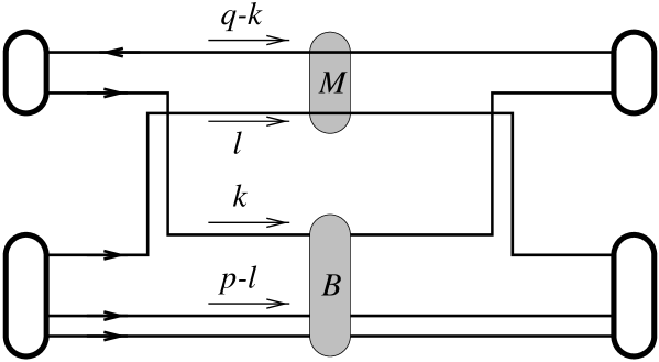
Figure 9: The intermediate rearrangement for light quarks is determined by the momenta of the collison partners as calculated in Eq. (34).

For the present discussion, we restore the internal degrees of freedom of the proton, i.e., the cross section envisaged here is written as in Ref. [3] with the full dependence on transverse and light cone coordinates of the quarks in both the photon and the proton.

$$\sigma_{\gamma^{*}p}=2\int d^{2}{\bf b}\int{dz_{1}d^{2}{\bf r}_{1}\over 4\pi}|\psi_{\gamma}(z_{1},{\bf r}_{1})|^{2}\int{dz_{2}d^{2}{\bf r}_{2}\over 4\pi}|\psi_{p}(z_{2},{\bf r}_{2})|^{2}\,J({\bf x}_{1},{\bf x}_{\bar{1}},{\bf x}_{2},{\bf x}_{\bar{2}})\Theta(z_{1},z_{2},W),$$ (35)

where 1 and 2 refer to the photon and nucleon sides, respectively. The proton is considered in a simple quark-diquark picture which has proved to be a good approximation in the framework of the stochastic vacuum model. In Eq. (35), we have inserted the threshold factor $\Theta$ which realizes the requirement of Eq. (34):

$$\Theta(z_{1},z_{2},W)=\theta\Big{[}z_{1}(1-z_{2})W^{2}-M_{B}^{2}\Big{]}\,\theta\Big{[}(1-z_{1})z_{2}W^{2}-M_{M}^{2}\Big{]}.$$ (36)

In the integrand of Eq. (23), the effect of the threshold factor is to generate a $z\equiv z_{1}$ dependent phase space factor:

$$\Phi(z)=\int_{0}^{1}dz_{2}\,f(z_{2})\,\theta\left[1-{M_{1}^{2}\over zW^{2}}-z_{2}\right]\,\theta\left[z_{2}-{M_{2}^{2}\over(1-z)W^{2}}\right].$$

In the integral, $f(z_{2})$ represents the $z_{2}$ dependence as it results for the various term in Eq. (35). Indeed, since the $z_{2}$ dependence of the quantity $J$ is rather weak, $f(z_{2})$ turns out to be given essentially by the square of the proton wave function, for which we use $f(z_{2})=252z_{2}^{2}(1-z_{2})^{6}$. For large energies, $W\gg M_{M}+M_{B}$, $\Phi(z)=1$ for intermediate $z$ and rapidly decreases to 0 when $z$ approaches the boundaries which at large enough $W$ read

$${M_{B}^{2}\over W^{2}}\leq z\leq 1-{M_{M}^{2}\over W^{2}}.$$

For $M_{B}=M_{p}$, $M_{M}=M_{\rho}$ and $W=20$ GeV, the boundaries are approximately $0.0022\leq z\leq 0.9985$.

The threshold factor is therefore important in case where the endpoint contribution is sizeable. Usual hadron wave functions suppress this region in both hadron-hadron collisions and vector meson production, thus rendering this effect unimportant at large energy, $s\geq 100$ GeV². In inclusive photon-hadron scattering, however, this endpoint region cannot be overlooked. The importance of the various region in $z$, in the full integral Eq. (23), may be studied by varying the lower limit $Z$ of the integration over quark light cone momenta in the photon wave function. Recall that the threshold condition for light quarks gives a lower limit $z\geq 0.0022$ for $W=20$ GeV as calculated above and that this lower limit goes like $1/W^{2}$. Since the integrand is symmetric in $z$, the upper integration limit can be restricted to $z\leq 0.5$. The resulting function $I_{T}(Z)$

$$I_{T}(Z)=\int_{Z}^{0.5}dz\int_{0}^{\infty}rdr{\cal I_{T}}(z,r),$$

is shown in Fig. 10 for the transverse cross section.

Figure 10: Interaction amplitude, $I_{T}(Z)/I_{T}(0)$, at $Q^{2}=3$ GeV² as a function of the cut off $Z$ limiting the momentum fraction of quarks in the photon. The effective mass used in this computation is the one given in Eq. (21).

In order to understand what happens in the endpoint region, it is instructive to study the behavior of the amplitude for a simplified $J_{p}(z,r)$ behaving like $C\,r^{n}$ with $n=1$ or 2. Our actual $J_{p}$ is in some sense interpolating between those two choices, the power $n=2$ corresponding to the short distance dipole behavior already mentioned in Eq. (26). With such a simple dependence, one can perform the $r$-integral analytically:

$$\int rdr\,{\cal I}_{L} = K{4z^{2}(1-z)^{2}Q^{2}\over[z(1-z)Q^{2}+m^{2}]^{1+n/2}},$$ (37)

$$\int rdr\,{\cal I}_{T} = K{(1+2/n)[z^{2}+(1-z)^{2}]\over[z(1-z)Q^{2}+m^{2}]^{n/2}}+K{m^{2}\over[z(1-z)Q^{2}+m^{2}]^{1+n/2}},$$ (38)

where the overall constant is

$$K={N_{c}C\over 4\pi^{2}}2^{n-1}{\Gamma^{4}(1+n/2)\over(n+1)!}.$$

For $m^{2}\ll Q^{2}$, one can focus on the first term in Eq. (38). At $Z\to 0$, the quantity $Q^{n}I_{T}(Z)$ behaves, for $n=2$, like

$$Q^{2}I_{T}(Z)\propto O(1)-\ln[Z+m^{2}/Q^{2}],$$

and, for $n=1$, like

$$Q\,I_{T}(Z)\propto O(1)-\sqrt{Z+m^{2}/Q^{2}}.$$

In Fig. 10, we see the transition from the logarithmic behavior given in case $n=2$ to a linear behavior at very small $Z$. The limit $Z=0$ is however approached like in the case $n=1$: it does not have the dramatic dependence on $m^{2}$ exhibited by the $n=2$ case. For $Q^{2}\leq 4m^{2}$, the integrands become more or less flat in $z$ and the $Z$ behavior is linear in the whole range.

Because the photon size parameter, $\varepsilon^{2}=z(1-z)Q^{2}+m^{2}$, is the important scale in $\cal I$, the behavior changes in the neighborhood of $Z=m^{2}/Q^{2}$. The region where the threshold suppression in photon-proton collisions is sizeable is therefore given by

$$m^{2}/Q^{2}\raisebox{-2.15277pt}{\footnotesize$\,\>\stackrel{{\scriptstyle\textstyle<}}{{\sim}}\,\>$}M^{2}/W^{2},$$

i.e.,

$$m^{2}/M^{2}\raisebox{-2.15277pt}{\footnotesize$\,\>\stackrel{{\scriptstyle\textstyle<}}{{\sim}}\,\>$}x_{B}.$$

For $M=M_{p}$ and $W=10$ GeV, this shows that the effect becomes sizeable when $Q^{2}\geq 0.5$ GeV², for an effective quark mass $\sim 0.1$ GeV. If we were to consider a current quark mass below this value of $Q^{2}$, the effect would show up at even a much smaller value of $Q^{2}$.

5.2 Threshold effect in the cross section

We now compare with data our computed cross section modified by the threshold effects from slow quarks. For photoproduction, the change is negligible. For electroproduction, it is best to consider fixed $Q^{2}$ and vary the energy $W$ to see the threshold effect. In Fig. 11 we show the variation of $F_{2}$ for 9 GeV$\leq W\leq 25$ GeV separately for $Q^{2}=1$, 3 and 9 GeV². (For convenience we shifted downward the first two sets by respectively $0.25$ and $0.15$.) We have checked that for these values of $Q^{2}$ the inclusion of the Reggeon contribution given in Ref. [8] only modifies weakly the trend of our curves for $W>10$ GeV. In each case we present results combining $u$, $d$ and $s$ contributions for both schemes: $z$ dependent quark masses, Eqs. (21) and (22), and $z$ independent quark masses, Eqs. (18) and (19). The effect is relatively stronger for the latter scheme since the endpoint contributions are clearly more important in this case. The difference between the two schemes decreases at small $W$ where only intermediate $z$ are taken into account. As anticipated the threshold effect is also more important at large $Q^{2}$ and at $Q^{2}=9$ GeV² the suppression of the cross section is typically 10% at $W=20$ GeV and reaches 30% at $W=10$ GeV. At this high $Q^{2}$ the effective quark mass has practically gone to zero in both schemes and the large distances are cut off by the threshold condition.

Figure 11: Contribution of $u$, $d$ and $s$ to $F_{2}$ as a function of $W$, for $Q^{2}=$1, 3 and 9 GeV², from bottom to top ($0.25$ has been substracted to the first set and $0.15$ to the second). The solid lines represent our result for $z$ dependent effective masses and the dashed lines correspond to $Q^{2}$ dependent effective masses. Squares are NMC results [9] and diamonds are E665 [10].

To complete our study we give in Fig. 12 our result for $F_{2}(x_{B}=Q^{2}/W^{2},Q^{2})$ at $W=20$ GeV including the threshold effect. The plot may be compared with Fig. 8 and we see that the qualitative aspect of the transition from low to high $Q^{2}$ remains. In general the large $Q^{2}$ range is sensitive to the threshold effect whereas the small $Q^{2}$ range tests more the effective quark mass.

Figure 12: Contribution of $u$, $d$ and $s$ to $F_{2}$ as a function of $Q^{2}$, for $W=$20 GeV. Curves and data are as in Fig. 8

6 Discussion and Conclusions

We have computed the total photon proton cross section in a model of nonperturbative QCD. For values of the virtual photon mass $Q^{2}>2$ GeV² our input is the treatment of two Wilson loops in Minkowski space-time within a special model of nonperturbative QCD which approximates the infrared behavior by a Gaussian stochastic process determined by a non-local gauge invariant gluon field correlator. The latter one is essentially given by the local gluon condensate and the correlation length. In order to fix the size distribution of one loop a proton valence quark wave function has to be introduced. In principle all parameters of the model can be determined by sources other than high energy scattering, namely lattice gauge calculations and low energy phenomenology. In practice the errors in the parameters still necessitate some adjustment to high energy scattering data. In our case we have chosen the determination of Ref. [3] based on the proton-proton total cross section and the logarithmic slope of the elastic $pp$ cross section at zero momentum transfer. Although the parameters turn out to be rather stable there remains still a certain variation in a range of a few percent for the correlation length and 20–30% for the gluon condensate and the proton radius. The model gives energy independent cross sections, contrary to the slight $s^{0.08}$ energy dependence seen in low $Q^{2}$ experiments. Since the parameters are related to the ISR energies, $W\approx 20$ GeV, we also compare the photon cross sections calculated here with experimental values around that energy. We have already used this procedure in order to calculate diffractive electroproduction of vector mesons with very good results.

In the present work we have extented the $Q^{2}$ range down to $Q^{2}=0$. In order to do that we have constructed nonperturbative photon wave functions essentially by introducing a virtuality dependent constituent quark mass. We were encouraged to such a simple procedure by model investigations of harmonic oscillator Green functions. In our method we adjusted the value of the momentum dependent quark mass to reproduce the phenomenological two point function of the vector currents. The development of a quark mass at large distances has been seen also in calculations with the instanton liquid model [11]. We repeat that none of our input parameters was in any way related or adjusted to electroproduction phenomenology.

Our approach differs in several ways from other investigations. For the treatment of the soft exchanges, Nikolaev and Zakharov have adopted a phenomenological two-gluon-exchange model [7]. Their treatment also gives importance to the $q\bar{q}$ photon wave function and their dipole-proton cross section has a $r^{2}$ behavior at short distance and saturates in the $r=1$–2 fm region. To suppress the contribution from large distance in the photon wave function they cut off the large size component using a smooth gaussian $\exp(-r^{2}/R_{c}^{2})$ with a confinement size parameter $R_{c}\approx 1.5\,$fm. In Ref. [7], a current quark mass $m_{u,d}=10$ MeV was used, but in a later study of the same authors on the BFKL pomeron [12] a constant light quark mass $m_{u,d}=150$ MeV was considered. As we have seen in our study such a value can help to limit the extent of the photon wave function, but at large $Q^{2}$ there is no reason that the light quarks have masses different from the current quark masses. In the region of transverse distance probed, we have seen that the nonperturbative features of the gluon correlators are important and we think that a perturbative two-gluon exchange model cannot be trusted.

Concerning the transition to small $Q^{2}$, we have shown an approach different from vector meson dominance (VMD) frequently used in the low $Q^{2}$ range. We claim that with increasing $Q^{2}$ one would have to put a rapidly growing number of resonances into the VMD model which thereby becomes untractable. Our scheme of quark-hadron duality exploits the knowledge about the residue and the mass of the lowest vector meson state contributing to the vector current two-point function.

Based on the transition between a VMD description of $F_{2}$ at small $Q^{2}$ and the partonic one at large $Q^{2}$ Badelek and Kwieciński have proposed to represent the proton structure function via dispersion relation [13]. The construction adopted here shares similarities with their approach although the latter makes no connexion to the notion of wave function which we need for the microscopic description of diffractive scatterings. In their approach the partonic contribution to $F_{2}$ is extracted from structure function analysis at large $Q^{2}$ and thus naturally fulfills perturbative QCD evolution at large virtualities where this evolution is experimentally observed. Such perturbative corrections are not implemented in our approach.

Our results are encouraging. Without any adjustment they agree with experiments over the full $Q^{2}$ range from 0 to 20 GeV² within 10–20%. For the high $Q^{2}$ range we have shown how finite energy corrections may account for at least a part of the discrepancy without changing any of the model parameter and without affecting the good description of the transition region where the modification of the perturbative $q\bar{q}$ wave function is at work. It is rather difficult to decide with present data what is the best scheme in our approach, i.e., whether or not the effective mass depends on the quark light cone fraction. In order to put our result in a larger perspective, we show in Fig. 13 the curve one deduces from Fig. 12 with the z independent masses, Eqs. (18) and (19), if we adjust the normalization by $-$10% (which would amount, e.g., to a 5% reduction of the gluon condensate). A rescaling of the curve in Fig. 8 by $-$15% shows the same pattern. We describe almost perfectly the $Q^{2}$ dependence of the data in the whole $Q^{2}$ range examined. This points toward the possibility that the chiral transition is already seen in present data, the kink in the data at $Q^{2}=1$ GeV² being related to the vanishing of the quark mass at that value of $Q^{2}$ (chiral restoration). The photon-proton cross section could also be easily adjusted by a slight decrease of the constituent quark mass.

Because of the fundamental importance of chiral symmetry breaking for hadron physics, the question of chiral symmetry restoration with increasing virtuality $Q^{2}$ of the photon deserves to be studied in more detail. More systematic data for $F_{2}(x_{B},Q^{2})$ and $F_{L}(x_{B},Q^{2})$ at fixed $W$ and varying $Q^{2}$ would help in deciding whether a marked change occurs between the low momentum domain and the perturbative domain in inelastic electron scattering. It may be that chiral symmetry restoration is seen more easily in electroproduction at a given virtuality $Q_{0}^{2}$ than in heavy ion collisions at a finite temperature $2\pi T=Q_{0}$.

Figure 13: Contribution of $u$, $d$ and $s$ to $F_{2}$ as a function of $Q^{2}$, for $W=20$ GeV. The curve is the result shown in Fig. 12 and for the $Q^{2}$ dependent quark masses of Eqs. (18) and (19) (dashed curve in Fig. 12) multiplied by $0.9$. This rescaling would correspond to a 5% decrease of the gluon condensate. Data are as in previous figures.

We thank B. Kopeliovich, G.Kulzinger, O. Nachtmann and M. Rueter for critical discussions. T. G. was carrying out his work as part of a training Project of the European Community under Contract No. ERBFMBICT950411. This work has been partially funded through the European TMR Contract No. FMRX-CT96-0008: Hadronic Physics with High Energy Electromagnetic Probes, and through DOE grant No. 85ER40214.

References

- [1] T.H. Bauer, F.M. Pipkin, R.D. Spital, and D.R. Yennie, Rev. Mod. Phys. 50, 261 (1978).
- [2] H.G. Dosch, E. Ferreira and A. Krämer, Phys. Rev. D 50, 1992 (1994).
- [3] H.G. Dosch, T. Gousset, G. Kulzinger and H.J. Pirner, Phys. Rev. D 55, 2602 (1997).
- [4] H.D. Politzer, Nucl. Phys. B117, 397 (1976).
- [5] M.A. Shifman, A.I. Vainshtein and V.I. Zakharov, Nucl. Phys. B147, 385 (1979).
- [6] J.D. Bjorken, J.B. Kogut and D.E. Soper, Phys. Rev. D 3, 1382 (1971).
- [7] N.N. Nikolaev and B.G. Zakharov, Z. Phys. C 49, 607 (1991).
- [8] A. Donnachie and P.V. Landshoff, Z. Phys. C 61, 139 (1994).
- [9] NMC, M. Arneodo et al., Nucl. Phys. B483, 3 (1997).
- [10] E665 collab., M.R. Adams et al., Phys. Rev. D 54, 3006 (1996).
- [11] E.V. Shuryak, Nucl. Phys. B328, 85 (1989).
- [12] N.N. Nikolaev and B.G. Zakharov, Phys. Lett. B333, 250 (1994).
- [13] B. Badelek and J. Kwieciński, Phys. Lett. B 295, 263 (1992).