We investigate numerical solution of Dokshitzer-Gribov-Lipatov-Altarelli-Parisi
(DGLAP) $Q^{2}$ evolution equations for longitudinally polarized structure functions. Flavor nonsinglet and singlet equations with next-to-leading-order $\alpha_{s}$ corrections are studied. A brute-force method is employed. Dividing the variables $x$ and $Q^{2}$ into small steps, we simply solve the integrodifferential equations. Numerical results indicate that accuracy is better than 1% in the region $10^{-5}<x<0.8$ if more than two-hundred $Q^{2}$ steps and more than one-thousand $x$ steps are taken. Our evolution results are compared with polarized experimental data of the spin asymmetry $A_{1}$ by the SLAC-E130, SLAC-E143, EMC, and SMC collaborations. The comparison indicates that we cannot assume $A_{1}$ is independent of $Q^{2}$. We provide a FORTRAN program for the Q² evolution and devolution of polarized nonsinglet-quark, singlet-quark, $\Delta q_{i}+\Delta\bar{q}_{i}$, and gluon distributions (and corresponding structure functions).

 

* Email: 96sm18@edu.cc.saga-u.ac.jp, kumanos@cc.saga-u.ac.jp, and

96td25@edu.cc.saga-u.ac.jp. Information on their research is available

at http://www.cc.saga-u.ac.jp/saga-u/riko/physics/quantum1/structure.html.

published as Comput. Phys. Commun. 108 (1998) 38.

Program Summary

Title of program: BFP1

Computer: AlphaServer 2100 4/200; Installation: The Research Center for Nuclear Physics in Osaka

Operating system: OpenVMS V6.1

Programming language used: FORTRAN 77

Peripherals used: Laser printer

No. of lines in distributed program, including test data, etc.: 1617

Keywords: Structure function, polarized parton distribution, Q² evolution, numerical solution.

Nature of physical problem

This program solves DGLAP $Q^{2}$ evolution equations with or without next-to-leading-order $\alpha_{s}$ effects for longitudinally polarized parton distributions. The evolved distributions could be convoluted with coefficient functions for calculating the structure function $g_{1}$. Both flavor-nonsinglet and singlet cases are provided, so that the distributions, $x\Delta q_{{}_{NS}}$, $x\Delta q_{{}_{S}}$, $x\Delta q_{i}^{+}\equiv x\Delta q_{i}+x\Delta\bar{q}_{i}$ ($i$=quark flavor), $x\Delta g$, $xg_{1_{NS}}$, $xg_{1_{S}}$, and $xg_{1,i}^{+}$ can be obtained.

Method of solution

The DGLAP integrodifferential equations are simply solved by a brute-force method. We divide the variables $x$ and $Q^{2}$ into very small steps, and the integrodifferential equations are solved step by step.

Restrictions of the program

This program is used for calculating Q² evolution of a longitudinally polarized flavor-nonsinglet-quark, singlet-quark, $\Delta q_{i}^{+}$, and gluon distributions in the leading order or in the next-to-leading order of $\alpha_{s}$. $Q^{2}$ evolution equations are the DGLAP equations. The double precision arithmetic is used. The renormalization scheme is the modified minimal subtraction scheme ($\overline{MS}$). A user provides the initial distribution as a subroutine or as a data file. Examples are explained in section 4. Then, the user inputs fifteen parameters in section 4.

Typical running time

Approximately seven minutes on AlphaServer 2100 4/200 in the nonsinglet case, sixty minutes in the singlet-quark evolution.

LONG WRITE-UP

1 Introduction

Spin structure of the proton has been investigated by polarized lepton-proton scattering. In particular, the structure function $g_{1}$ provides us information on the probability to find a quark polarized along the direction of longitudinally polarized proton spin minus the one polarized oppositely. Experimentally, it is measured by a spin asymmetry in the lepton-proton scattering. The $g_{1}$ is a function of two kinematical variables $Q^{2}$ and $x=Q^{2}/(2p\cdot q)$, where $p$ is the proton momentum and $Q^{2}$ is given by the four-momentum transfer $q$ as $Q^{2}=-q^{2}$. The $x$ dependence is associated with nonperturbative physics, so that $x$ distributions of polarized parton distributions are obtained by fitting various experimental data. At this stage, the only way to study the parton $x$ distributions theoretically is to use phenomenological quark models. On the other hand, the $Q^{2}$ dependence is well predicted in perturbative QCD. In general, structure functions are almost independent of the scale $Q^{2}$, which is called Bjorken scaling. However, even though it is small, scaling-violation phenomena are observed. The experimental data support perturbative QCD predictions.

As a way of describing the scaling violation, Dokshitzer-Gribov-Lipatov-Altarelli-Parisi (DGLAP) equations [1] are usually used. They are coupled integrodifferential equations. Because the DGLAP equations are frequently used in theoretical and experimental studies, it is worth while creating a program to solve them accurately. We have been studying this topic last several years in a Laguerre-polynomial method [2] and in a brute-force method [3, 4]. Here, we extend the studies to the spin-dependent case. Fortunately, the next-to-leading-order (NLO) splitting functions are calculated recently for polarized parton distributions [5]. It enables us to investigate the details of NLO effects on the $Q^{2}$ evolution. We create a FORTRAN program for obtaining numerical solution of the polarized DGLAP equations with the NLO effects. With our program, $Q^{2}$ evolution of nonsinglet quark, singlet quark, and gluon distributions can be obtained. Furthermore, NLO coefficient functions could be convoluted with the evolved distributions in our program for calculating the $g_{1}$ structure function. It is very useful for investigating polarized parton distributions. In fact, our program in a slightly modified form is used for investigating optimum polarized parton distributions by fitting experimental data [6].

We explain the details of our studies in the following. In section 2, the polarized DGLAP $Q^{2}$ evolution equations are explained. Then, our numerical solution method is described in section 3. Input parameters and input distributions are discussed in section 4, and essential subroutines in the program are explained in section 5. Numerical results and their comparison with experimental data are discussed in section 6. Summary is given in section 7. Explicit forms of splitting functions and the coefficient functions are listed in Appendices.

2 $\bf Q^{2}$ evolution equations

We use the DGLAP equations [1] for studying the $Q^{2}$ evolution. Both the leading order (LO) and the next-to-leading order (NLO) cases can be handled by the DGLAP equations. NLO effects are included in the running coupling constant $\alpha_{s}(Q^{2})$ and in the splitting functions $\Delta P_{ij}(x)$. Here, the evolution of polarized parton distributions $\Delta q=q_{\uparrow}-q_{\downarrow}$ and $\Delta g=g_{+1}-g_{-1}$ is investigated.

First, the nonsinglet DGLAP equation is given by

$$\frac{\partial}{\partial\ln Q^{2}}\,\Delta q_{{}_{NS}}(x,Q^{2})\ =\frac{\alpha_{s}(Q^{2})}{2\pi}\ \Delta P_{q^{\pm},{NS}}(x)\otimes\Delta q_{{}_{NS}}(x,Q^{2})\ ,$$ (2.1)

where $\Delta q_{{}_{NS}}(x,Q^{2})$ is a polarized nonsinglet parton distribution, $\Delta P_{q^{\pm},{NS}}$ is the polarized nonsinglet splitting function, and the convolution $\otimes$ is defined by

$$f(x)\otimes g(x)=\int^{1}_{x}\frac{dy}{y}f\left(\frac{x}{y}\right)g(y)\ .$$ (2.2)

The notation $q^{\pm}$ in the splitting function indicates a $\Delta q^{+}=\Delta q+\Delta\bar{q}$ or $\Delta q^{-}=\Delta q-\Delta\bar{q}$ distribution type, which is explained in Appendix A. Instead of $Q^{2}$, it is more convenient to use the variable $t$ defined by

$$t\equiv-\frac{2}{\beta_{0}}\ln\left[\frac{\alpha_{s}(Q^{2})}{\alpha_{s}(Q_{0}^{2})}\right]\ ,$$ (2.3)

where $\beta_{0}$ is defined in Appendix A. The parton distribution and the splitting function multiplied by $x$

$$\widetilde{f}(x)=xf(x)$$ (2.4)

satisfy the same integrodifferential equation. Therefore, we rewrite the evolution equation as

$$\frac{\partial}{\partial t}\ \Delta\widetilde{q}_{{}_{NS}}(x,t)=\Delta\widetilde{P}_{q^{\pm},{NS}}(x)\otimes\Delta\widetilde{q}_{{}_{NS}}(x,t)\ .$$ (2.5)

Next, the singlet evolution is more complicated than the nonsinglet one due to gluon participation in the evolution. The singlet quark distribution is defined by $\Delta\widetilde{q}_{s}(x,t)\equiv\sum_{i}^{N_{f}}x\,\Delta q_{i}^{+}$ where $i$ is the flavor, and $\Delta\widetilde{g}(x,t)$ is the gluon distribution. The singlet case is given by

$$\frac{\partial}{\partial t}\left(\begin{array}[]{c}\Delta\widetilde{q}_{s}(x,t)\\ \Delta\widetilde{g}(x,t)\end{array}\right) = \left(\begin{array}[]{cc}\Delta\widetilde{P}_{qq}(x,t)&\Delta\widetilde{P}_{qg}(x,t)\\ \Delta\widetilde{P}_{gq}(x,t)&\Delta\widetilde{P}_{gg}(x,t)\\ \end{array}\right)\otimes\left(\begin{array}[]{c}\Delta\widetilde{q}_{s}(x,t)\\ \Delta\widetilde{g}(x,t)\end{array}\right)\ .$$ (2.12)

If each flavor evolution is necessary, another equation has to be used in addition to Eq. (2.12). Using the properties of the splitting functions, $\Delta\widetilde{P}^{(1)}_{q^{+}_{i}q^{+}_{j}}=\delta_{ij}\,\Delta\widetilde{P}^{(1)}_{q^{+},_{NS}}+2C_{F}T_{R}\widetilde{F}_{qq}$ and $\Delta\widetilde{P}^{(1)}_{q^{+}_{j}g}=\Delta\widetilde{P}^{(1)}_{q^{+}g}$ (independent of $j$), we have the evolution equation

$$\frac{\partial}{\partial t}\Delta\widetilde{q}_{i}^{\,+}(x,t)=\Delta\widetilde{P}_{q^{+},\,_{NS}}(x)\otimes\Delta\widetilde{q}_{i}^{\,+}(x,t) +\ 2\,C_{F}\,T_{R}\,\widetilde{F}_{qq}(x)\otimes\Delta\widetilde{q}_{{}_{S}}(x,t)$$

$$+\Delta\widetilde{P}_{q_{i}^{+}g}(x)\otimes\Delta\widetilde{g}(x,t)\ .$$ (2.13)

In this case, three coupled integrodifferential equations in Eqs. (2.12) and (2.13) should be solved simultaneously. All the necessary splitting functions $\Delta\tilde{P}$ and $\tilde{F}$ are listed in Appendix A.

We discuss the NLO effects in the evolution equations. The NLO contributions are included in the running coupling constant $\alpha_{s}(t)$, in the splitting functions $\Delta P_{ij}(z)$, and in the coefficient functions. Once the NLO corrections are included in the evolution, the renormalization scheme has to be specified. We use the $\overline{MS}$ scheme throughout this paper.

The running coupling constant in the leading order (LO) is given by

$$\alpha_{s}^{LO}(Q^{2})=\frac{4\pi}{\beta_{0}\ln(Q^{2}/\Lambda^{2})}\ ,$$ (2.14)

and the one in the next-to-leading order (NLO) is

$$\alpha_{s}^{NLO}(Q^{2})=\frac{4\pi}{\beta_{0}\ln(Q^{2}/\Lambda^{2})}\left[1-\frac{\beta_{1}\ln\{\ln(Q^{2}/\Lambda^{2})\}}{\beta_{0}^{2}\ln(Q^{2}/\Lambda^{2})}\right]\ .$$ (2.15)

The constants $\beta_{0}$ and $\beta_{1}$ are defined in Appendix A. The splitting functions have the perturbative-expansion form

$$\Delta P_{ij}(x)=\Delta P_{ij}^{(0)}(x)+\frac{\alpha_{s}(Q^{2})}{2\pi}\,\Delta P_{ij}^{(1)}(x)\ .$$ (2.16)

The second term is the NLO contributions to the splitting functions. The functions are expressed by the ones multiplied by $x$ ($\Delta\widetilde{P}$). Changing the variable $Q^{2}$ to $t$ in the DGLAP equations, we have the splitting functions

$$\Delta\widetilde{P}_{ij}(x)=\Delta\widetilde{P}_{ij}^{(0)}(x)+\frac{\alpha_{s}(t)}{2\pi}\Delta R_{ij}(x)\ ,$$ (2.17)

where the function $\Delta R_{ij}(x)$ is

$$\Delta R_{ij}(x)\equiv\Delta\widetilde{P}_{ij}^{(1)}(x)-\frac{\beta_{1}}{2\beta_{0}}\,\Delta\widetilde{P}_{ij}^{(0)}(x)\ .$$ (2.18)

The second term in Eq. (2.18) appears because of the transformation from $Q^{2}$ to $t$. To be precise, the splitting functions $\Delta\widetilde{P}_{ij}$ in Eq. (2.17) should be denoted, for example, $\Delta\widetilde{P}_{ij}^{\prime}$ because it is different from $x\Delta P_{ij}=x\Delta P_{ij}^{(0)}+(\alpha_{s}/2\pi)x\Delta P_{ij}^{(1)}$ which is Eq. (2.16) multiplied by $x$. (Note the definition of $\tilde{f}$ is $\tilde{f}=xf$.) However, we use the expression without the prime throughout this paper for simplicity. We have the same expression $\Delta\widetilde{P}_{NS}=\Delta\widetilde{P}^{(0)}_{NS}+\alpha_{s}/(2\pi)\Delta R_{NS}$ in the nonsinglet case.

Next, we discuss the spin-dependent structure function $g_{1}$. We have discussed how the $Q^{2}$ evolution of quark and gluon distributions is described. However, these parton distributions are not observed directly in experiments. The $g_{1}$ could be measured in the polarized lepton-proton scattering with information on the unpolarized structure function $F_{1}$. In the LO case, it is given in parton model as

$$xg_{1}(x)=\frac{1}{2}\sum_{i}^{N_{f}}e^{2}_{i}\,\Delta\widetilde{q}_{i}^{\,+}(x)\ .$$ (2.19)

The NLO effects in the structure function are included in the coefficient functions and also in the quark and gluon distributions. In the NLO case, the quark distributions should be convoluted with a coefficient function. Furthermore, an additional gluon correction term should be taken into account:

$$xg_{1}(x)=\frac{1}{2}\sum_{i}^{N_{f}}e^{2}_{i}\,\left[\,\Delta\widetilde{C}_{q}(x)\otimes\Delta{\widetilde{q}}_{i}^{\,+}(x)+\Delta\widetilde{C}_{g}(x)\otimes\Delta\widetilde{g}(x)\,\right]\ ,$$ (2.20)

where $\Delta\widetilde{C}_{q}/x$ and $\Delta\widetilde{C}_{g}/x$ are the quark and gluon coefficient functions in Appendix B. The calculation procedure for the $g_{1}$ evolution is the following. First, the $Q^{2}$ evolution of the quark and gluon distributions is calculated. Then, the structure function $g_{1}$ at $Q^{2}$ is evaluated by using Eq. (2.19) or (2.20). An example is explained in section 6.2.

3 Brute-force method

Among various methods of solving the DGLAP equations, we decide to employ a brute-force method. So far, we have investigated two methods, the Laguerre-polynomial [2] and the brute-force [3] methods, in the spin-independent case. The Laguerre method has an advantage of computing time. However, numerical accuracy becomes slightly worse in the nonsinglet case at small $x$. As far as we studied, the situation is better in the polarized distributions. However, we find a tendency that the accuracy is slightly worse at small $x$. In light of future HERA spin physics, our program should be accurately enough even at $x=10^{-5}$. Therefore, we consider that the brute-force method is safer for getting accurate results in the wide $x$ range. The variables $x$ and $t$ are divided into small steps, then integration and differentiation are defined by

$$\frac{df(x)}{dx} =\frac{f(x_{m+1})-f(x_{m})}{\delta x_{m}}\ ,$$ (3.1)

$$\int f(x)\ dx =\sum_{m=1}^{N_{x}}\delta x_{m}f(x_{m})\ .$$ (3.2)

With these replacements, the evolution equations could be solved rather easily. For example, Eq. (2.5) is written in the following form:

$$\Delta\widetilde{q}_{{}_{NS}}(x_{k},t_{j+1})=\Delta\widetilde{q}_{{}_{NS}}(x_{k},t_{j})+\delta t_{j}\,\sum_{m=k}^{N_{x}}\frac{\delta x_{m}}{x_{m}}\,\Delta\widetilde{P}_{q^{\pm},NS}\left(\frac{x_{k}}{x_{m}}\right)\,\Delta\widetilde{q}_{{}_{NS}}(x_{m},t_{j})\ .$$ (3.3)

First, the evolution from $t_{0}=0$ to $t_{1}=\delta t$ is calculated in the above equation by providing the initial distribution ${\Delta\widetilde{q}}_{{}_{NS}}({x}_{m},{t}_{j=1})$. Repeating this step $N_{t}-1$ times, we obtain the final distribution at $t_{N_{t}}$. Accurate results cannot be obtained at small $x$ if the linear $x$ step is taken ($\delta x=1/N_{x}$). Therefore, the logarithmic-$x$ step $\delta(log_{10}x)=|log_{10}x_{min}|/N_{x}$ is taken in our evolution calculations.

The same method can be applied to the singlet and $\Delta q_{i}^{+}$ evolution equations in Eqs. (2.12) and (2.13). These equations are written in the brute-force method as:

$$\Delta\widetilde{q}_{i}^{\ +}(x_{k},t_{j+1})= \Delta\widetilde{q}_{i}^{\ +}(x_{k},t_{j})\,+\,\delta t_{j}\,\sum_{m=k}^{N_{x}}\frac{\delta x_{m}}{x_{m}}\,\Delta\widetilde{P}_{q^{+},NS}\left(\frac{x_{k}}{x_{m}}\right)\,\Delta\widetilde{q}_{i}^{\,+}(x_{m},t_{j})$$

$$+\,\delta t_{j}\,\sum_{m=k}^{N_{x}}\frac{\delta x_{m}}{x_{m}}\,2\,C_{F}\,T_{R}\,\widetilde{F}_{qq}\left(\frac{x_{k}}{x_{m}}\right)\,\Delta\widetilde{q}_{{}_{S}}(x_{m},t_{j})$$

$$+\,\delta t_{j}\,\sum_{m=k}^{N_{x}}\frac{\delta x_{m}}{x_{m}}\,\Delta\widetilde{P}_{q_{i}^{+}g}\left(\frac{x_{k}}{x_{m}}\right)\,\Delta\widetilde{g}(x_{m},t_{j})\ ,$$ (3.4a)

$$\Delta\widetilde{q}_{{}_{S}}(x_{k},t_{j+1})= \Delta\widetilde{q}_{{}_{S}}(x_{k},t_{j})\,+\,\delta t_{j}\,\sum_{m=k}^{N_{x}}\frac{\delta x_{m}}{x_{m}}\,\Delta\widetilde{P}_{qq}\left(\frac{x_{k}}{x_{m}}\right)\,\Delta\widetilde{q}_{{}_{S}}(x_{m},t_{j})$$

$$+\,\delta t_{j}\,\sum_{m=k}^{N_{x}}\frac{\delta x_{m}}{x_{m}}\,\Delta\widetilde{P}_{qg}\left(\frac{x_{k}}{x_{m}}\right)\,\Delta\widetilde{g}(x_{m},t_{j})\ ,$$ (3.4b)

$$\Delta\widetilde{g}(x_{k},t_{j+1})= \Delta{\widetilde{g}}({x}_{k},{t}_{j})\ +\ \delta t_{j}\,\sum_{m=k}^{N_{x}}\frac{\delta x_{m}}{x_{m}}\ \Delta\widetilde{P}_{gq}\left(\frac{x_{k}}{x_{m}}\right)\ \Delta\widetilde{q}_{{}_{S}}(x_{m},t_{j})$$

$$+\ \delta t_{j}\,\sum_{m=k}^{N_{x}}\frac{\delta x_{m}}{x_{m}}\ \Delta\widetilde{P}_{gg}\left(\frac{x_{k}}{x_{m}}\right)\ \Delta\widetilde{g}(x_{m},t_{j})\ .$$ (3.4c)

These are coupled equations. However, they can be solved by providing the initial distributions, $\Delta\widetilde{q}_{i}^{\,+}(x_{m},t_{j=0})\ ,\ \Delta\widetilde{q}_{{}_{S}}(x_{m},t_{j=0})$, and $\Delta\widetilde{g}(x_{m},t_{j=0})$, and by repeating the evolution step $N_{t}$ times.

We should be careful in handling $1/(1-x)_{+}$ terms in the splitting functions. They are given in our method by

$$\int_{x}^{1}dx^{\prime}\frac{f(x^{\prime})}{(1-x^{\prime})_{+}}=\sum_{m=k}^{N_{x}}\delta x_{m}\,\frac{f(x_{m})-f(1)}{1-x_{m}}\ +\ f(1)\,\ln(1-x_{k})\ .$$ (3.5)

In the same way, the integral with $[\ln(1-x)/(1-x)]_{+}$ becomes

$$\int_{x}^{1}dx^{\prime}f(x^{\prime})\left[\frac{\ln(1-x^{\prime})}{1-x^{\prime}}\right]_{+}= \sum\limits_{m=k}^{N_{x}}\delta x_{m}\,[f(x_{m})-f(1)]\,\frac{\ln(1-x_{m})}{1-x_{m}}$$

$$+\frac{1}{2}\,f(1)\,\ln^{2}(1-x_{k})\ .$$ (3.6)

4 Description of input parameters and input
distribution

For running the FORTRAN-77 program BFP1, a user should supply fifteen input parameters from the file #10. In addition, an input distribution(s) should be given in a function subroutine(s) in the end of the FORTRAN program or in an input data file(s), #13, #14, and/or #15. The initial distribution(s) could be written in the output file #12. Evolution results are written in the output file #11. We explain the input parameters and the input distributions in the following.

4.1 Input parameters

There are fifteen parameters. Numerical values of the parameters should be supplied in the file #10, then these are read in the main program.

IOUT	1	write $x$ and $x\Delta q_{{}_{NS}}(x)$ [or $xg_{1_{NS}}(x)$] at fixed $Q^{2}$ (=Q2) in the file #11
	2	write $Q^{2}$ and $x\Delta q_{{}_{NS}}(Q^{2})$ [or $xg_{1_{NS}}(Q^{2})$] at fixed $x$ (=XX) in the file #11
	3	$x$, $x\Delta q_{{}_{S}}(x)$ [or $xg_{1_{S}}(x)$], and $x\Delta g(x)$
	4	$Q^{2}$, $x\Delta q_{{}_{S}}(Q^{2})$ [or $xg_{1_{S}}(Q^{2})$], and $x\Delta g(Q^{2})$
	5	$x$, $x\Delta q_{i}^{+}(x)$ [or $xg_{1,i}^{+}(x)$], $x\Delta q_{{}_{S}}(x)$ [or $xg_{1_{S}}(x)$], and $x\Delta g(x)$ [or $xg_{1,g}(x)$]
	6	$Q^{2}$, $x\Delta q_{i}^{+}(Q^{2})$ [or $xg_{1,i}^{+}(Q^{2})$], $x\Delta q_{{}_{S}}(Q^{2})$ [or $xg_{1_{S}}(Q^{2})$],
		and $x\Delta g(Q^{2})$ [or $xg_{1,g}(x)$]
IREAD	1	give initial distribution(s) in function subroutine(s)
	2	read initial distribution(s) from data file(s)
INDIST	1	do not write initial distribution(s)
	2	write initial distribution(s) in the file #12
	3	write initial distribution(s) in the file #12 without calculating evolution
IORDER	1	leading order (LO) in $\alpha_{s}$
	2	next-to-leading order (NLO)
ITYPE	1	structure function $xg_{1}(x,Q^{2})$
	2	quark distribution $x\Delta q(x,Q^{2})$ and gluon distribution $x\Delta g(x,Q^{2})$
IMORP	1	$x\Delta q_{i}-x\Delta\bar{q}_{i}$ type distribution
	2	$x\Delta q_{i}+x\Delta\bar{q}_{i}$ type distribution

Q02	initial $Q^{2}$ ($\equiv Q_{0}^{2}$ in GeV2 ) at which an initial distribution is supplied
Q2	$Q^{2}$ to which the distribution is evolved ($Q^{2}\neq Q_{0}^{2}$, $Q^{2}>Q_{0}^{2}$ or $Q^{2}<Q_{0}^{2}$)
DLAM	QCD scale parameter $\Lambda_{QCD}$ in GeV
NF	number of quark flavors
XX	$x$ at which $Q^{2}$ dependent distributions are written (IOUT=2, 4, or 6 case)
NX	number of $x$ steps (NX$<$5000)
NT	number of $t$ steps (NT$<$5000)
NSTEP	number of $x$ steps or $t$ steps for writing output distribution(s)
NXMIN	$log_{10}$(minimum of $x$) $[0<min(x)=10^{{}^{NXMIN}}<XX]$

The meaning of IREAD is explained in section 4.2. The structure function $xg_{1}^{p}$ is obtained by the convolution of the distributions, $(1/2)[(4/9)x(\Delta u+\Delta\bar{u}+\Delta c+\Delta\bar{c})+(1/9)x(\Delta d+\Delta\bar{d}+\Delta s+\Delta\bar{s})]$ and $x\Delta g$ in the four flavor case, with the corresponding coefficient functions. Practically, we use the expression $(1/2)\sum_{i}e_{i}^{2}x\Delta q_{i}=(1/2)x[4\Delta q_{s}-3(\Delta d^{+}+\Delta s^{+})]/9$, where $\Delta d^{+}=\Delta d+\Delta\overline{d}$ and $\Delta s^{+}=\Delta s+\Delta\overline{s}$, instead of the above one in calculating $xg_{1}$. It is explained in more detail in section 6.2. The expression could be used only in the four and three flavor cases. In the five or six flavor evolution, it should be slightly modified. The parameter IMORP indicates a plus or minus type distribution $\sum_{i}a_{i}x(\Delta q_{i}\pm\Delta\bar{q}_{i})$, where $a_{i}$ are some constants. IMORP=1 or 2 should be taken in the nonsinglet evolution. In the singlet or $\Delta q_{i}^{+}$ case, IMORP=2 should be chosen.

For example, if one would like to evolve an initial singlet-quark distribution $x\Delta q_{{}_{S}}$ at $Q^{2}$=4 GeV² to the distribution at $Q^{2}$=200 GeV² by the NLO DGLAP equations with $N_{f}$=4 and $\Lambda$=0.231 GeV, the input parameters could be IOUT=3, IREAD=1, INDIST=1, IORDER=2, ITYPE=2, IMORP=2, Q02=4.0, Q2=200.0, DLAM=0.231, NF=4, XX=0.0, NX=1000, NT=200, NSTEP=100, and NXMIN=$-$4. In this case, the input file #10 is the following:

3, 1, 1, 2, 2, 2

4.0, 200.0, 0.231, 4, 0.0, 1000, 200, 100, $-$4  .

4.2 Input distributions supplied by function subroutines
(IREAD=1)

If IREAD=1 is chosen, an input distribution(s) at $Q_{0}^{2}$ should be supplied in the end of the FORTRAN program BFP1 as a function subroutine(s).

1) Nonsinglet case

An initial nonsinglet-quark distribution at $Q_{0}^{2}$ should be given in QNS0(X) as a double precision function. As an example, the GS (set A) valence quark distribution $x\Delta u_{v}+x\Delta d_{v}$ [7] at $Q_{0}^{2}$=4 GeV² is given in the program BFP1.

2) Singlet case

An initial singlet-quark distribution at $Q_{0}^{2}$ should be supplied in QS0(X), and an initial gluon distribution in the nucleon should be in G0(X). The GS $x\Delta q_{{}_{S}}=x\Delta u_{v}+x\Delta d_{v}+6x\Delta S$ and $x\Delta g$ distributions are given in the program.

3) $\Delta q_{i}^{+}$ distribution case

In addition to the above $x\Delta q_{{}_{S}}$ and $x\Delta g$ distributions, the initial $x\Delta q_{i}^{+}$ distribution (and another flavor distribution $x\Delta q_{j}^{+}$) should be supplied. In calculating two-flavor distributions simultaneously for obtaining $xg_{1}$, two distributions (e.g. $x\Delta d^{+}$ and $x\Delta s^{+}$) should be supplied in the functions QI0(1,x) and QI0(2,x). If one needs only one-flavor evolution, one may set QI0(2,x)=0. The GS distributions $x\Delta d^{+}$ and $x\Delta s^{+}$ are given in our program as an example.

4.3 Input distributions supplied by data files (IREAD=2)

If IREAD=2 is chosen, an input distribution(s) at $Q_{0}^{2}$ should be supplied in a separate data file(s).

1) Nonsinglet case (data file #13)

An initial nonsinglet-quark distribution at $Q_{0}^{2}$ should be given in the data file #13 as shown in the following example.

0.000100	0.009761
0.000110	0.010184
0.000120	0.010624
0.000132	0.011081
0.000145	0.011555
…	…
…	…
…	…
1.000000	0.000000

The first column is the $x$ values and the second one is the corresponding $x\Delta u_{v}+x\Delta d_{v}$ values. The data at $x\leq x_{min}$ and at $x$=1.0 must be supplied.

2) Singlet case in the nucleon (data file #14)

An initial singlet-quark distribution and a gluon distribution should be given in the data file #14 as shown in the following.

0.000100	0.001721	0.006729
0.000110	0.001612	0.007193
0.000120	0.001485	0.007688
0.000132	0.001339	0.008218
0.000145	0.001172	0.008784
…	…	…
…	…	…
…	…	…
1.000000	0.000000	0.000000

The first column is the $x$ values, the second is the $x\Delta q_{{}_{S}}$ distribution, and the third is the $x\Delta g$ distribution. The data at $x\leq x_{min}$ and at $x$=1.0 must be supplied.

3) $\Delta q_{i}^{+}$ distribution case (data file #15)

An initial $\Delta q_{i}^{+}$ distribution, a singlet-quark distribution, and a gluon distribution should be given in the data file #15 as shown in the following.

0.000100	-0.003637	-0.002681	0.001721	0.006729
0.000110	-0.003884	-0.002859	0.001612	0.007193
0.000120	-0.004147	-0.003048	0.001485	0.007688
0.000132	-0.004428	-0.003249	0.001339	0.008218
0.000145	-0.004727	-0.003462	0.001172	0.008784
…	…	…	…	…
…	…	…	…	…
…	…	…	…	…
1.000000	0.000000	0.000000	0.000000	0.000000

The first column is the $x$ values, the second is the $x\Delta q_{i}^{+}$ distribution, the third is another flavor distribution $x\Delta q_{j}^{+}$, the fourth is $x\Delta q_{{}_{S}}$, and the fifth is $x\Delta g$. The data at $x\leq x_{min}$ and at $x$=1.0 must be supplied. If one needs only one-flavor evolution, the second or third column values are set to 0.

5 Description of the program BFP1

The major part of the program BFP1 is essentially the same as the unpolarized version [3]. We do not explain each subroutine in this section. They are already well described in the previous publication, so that the interested reader may read Ref. [3] for the detailed description of all the subroutines.

The main program reads fifteen input parameters from the input file #10. Actual $Q^{2}$ evolution calculations are done by calling the subroutine GETQNS in the nonsinglet case and GETQS in the singlet (or $x\Delta q_{i}$) case. Each evolution step is calculated by the subroutine QNSXT or GETQGX. Minor modifications are made in each flavor evolution (GETQS) so that two quark distributions ($x\Delta q_{i}^{+}$ and $x\Delta q_{j}^{+}$) are evolved simultaneously. A typical function of the GS parton distributions is given as the function GS(X,A,B,C,D,E,F). We explain the subroutines associated with the input distributions in the following.

5.1 Function GS(X,A,B,C,D,E,F)

This function calculates the GS parton distributions given by the parameters A, B, C, D, E, and F as $ABx^{C}(1-x)^{D}(1+Ex+F\sqrt{x})$.

5.2 Functions QNS0(X), QS0(X), G0(X), and QI0(I,X)

The functions QNS0, QS0, and G0 calculate an initial nonsinglet-quark distribution $x\Delta q_{{}_{NS}}$, a singlet-quark distribution $x\Delta q_{{}_{S}}$, and a gluon distribution $x\Delta g$. As an example, the GS distributions [7] are provided.
The nonsinglet one is

$$QNS0= x\Delta u_{v}+x\Delta d_{v}$$

$$= 0.918*1.365x^{0.512}(1-x)^{3.96}(1+11.65x-4.6\sqrt{x})$$

$$+(-0.339)*3.849x^{0.78}(1-x)^{4.96}(1+7.81x-3.48\sqrt{x})\ ,$$ (5.1)

the singlet one in the three flavor case is

$$QS0= x\Delta u_{v}+x\Delta d_{v}+6x\Delta S$$

$$= 0.918*1.365x^{0.512}(1-x)^{3.96}(1+11.65x-4.6\sqrt{x})$$

$$+(-0.339)*3.849x^{0.78}(1-x)^{4.96}(1+7.81x-3.48\sqrt{x})$$

$$+6*(-0.06)*18.521x^{0.724}(1-x)^{14.4}(1+4.63x-4.96\sqrt{x})\ ,$$ (5.2)

and the gluon distribution is

$$G0=1.71*3.099x^{0.724}(1-x)^{5.71}(1+0.0x+0.0\sqrt{x})\ .$$ (5.3)

The function QI0 calculates two initial flavor distributions. As an example, the GS $x\Delta d^{+}=x\Delta d+x\Delta\overline{d}$ and $x\Delta s^{+}=x\Delta s+x\Delta\overline{s}$ distributions are provided:

$$QI0_{1}= x\Delta d_{v}+2x\Delta\bar{d}$$

$$= -0.339*3.849x^{0.78}(1-x)^{4.96}(1+7.81x-3.48\sqrt{x})$$

$$+2*(-0.06)*18.521x^{0.724}(1-x)^{14.4}(1+4.63x-4.96\sqrt{x})\ ,$$ (5.4)

$$QI0_{2}= 2x\Delta s$$

$$= 2*(-0.06)*18.521x^{0.724}(1-x)^{14.4}(1+4.63x-4.96\sqrt{x})\ .$$ (5.5)

In these equations, the flavor symmetry $\Delta\bar{u}=\Delta\bar{d}=\Delta\bar{s}=\Delta S$ is assumed.

6 Numerical analysis

6.1 Accuracy of $Q^{2}$ evolution results

There are two parameters which determine the accuracy of our numerical results. They are the numbers of steps: $N_{x}$ and $N_{t}$. As they become larger, the accuracy becomes better. However, there is a restriction because the evolution computation should be done within a certain CPU time depending on the machine power. We check how the evolution results depend on these parameters and how long it takes for finishing the evolution.

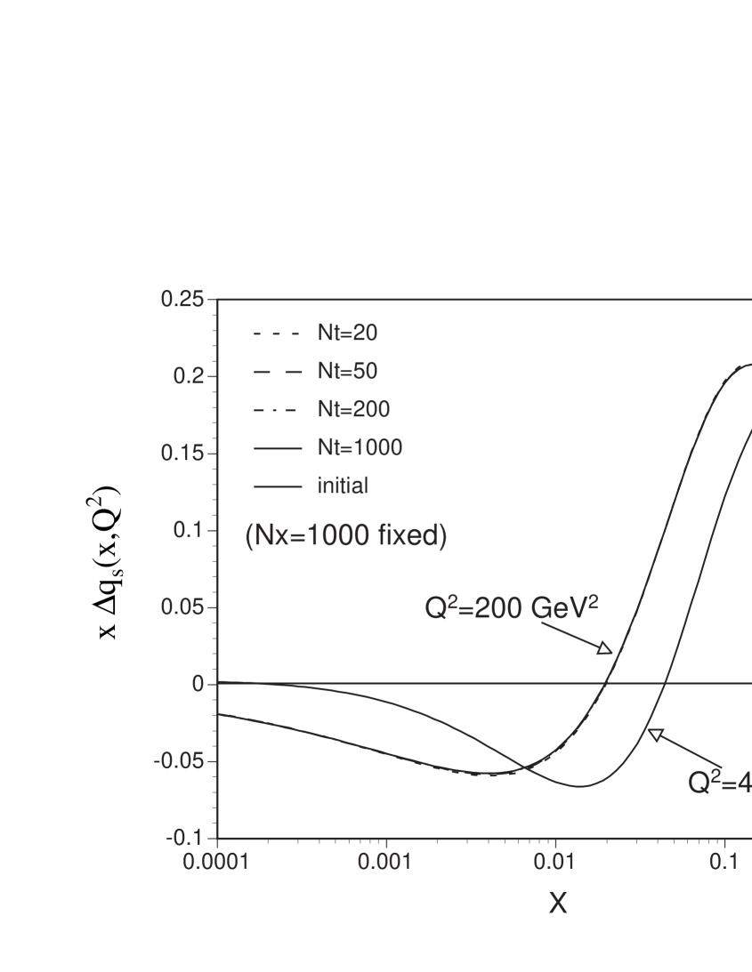
First, we fix the $x$ step at $N_{x}$=1000, then the $t$ step $N_{t}$ is varied as 20, 50, 200, and 1000. Numerical results for the polarized singlet quark distribution are shown in Fig. 1. The initial distribution is the GS-A at $Q^{2}$=4 GeV² [7]. The three-flavor distribution is considered. Because there is little information on each antiquark distribution [9], flavor symmetric distributions are assumed for the antiquark distributions. The scale parameter is taken as $\Lambda$=231 MeV in fitting polarized experimental data. We use $N_{f}=$4 and $\Lambda$=231 MeV for calculating the evolution. The GS-A singlet distribution is evolved to the one at $Q^{2}$=200 GeV² by our NLO program. The input distribution is supplied in the end of the program as the subroutine QS0. The input parameters are IOUT=3, IREAD=1, INDIST=1, IORDER=2, ITYPE=2, IMORP=2, Q02=4.0, Q2=200.0, DLAM=0.231, NF=4, XX=0.0, NX=1000, NT=200, NSTEP=100, and NXMIN=$-$4. There is almost no difference between the various results in Fig. 1, which means that merely fifty steps are enough for getting accurate evolution. This is certainly expected from the fact that the scaling violation is a small logarithmic effect.

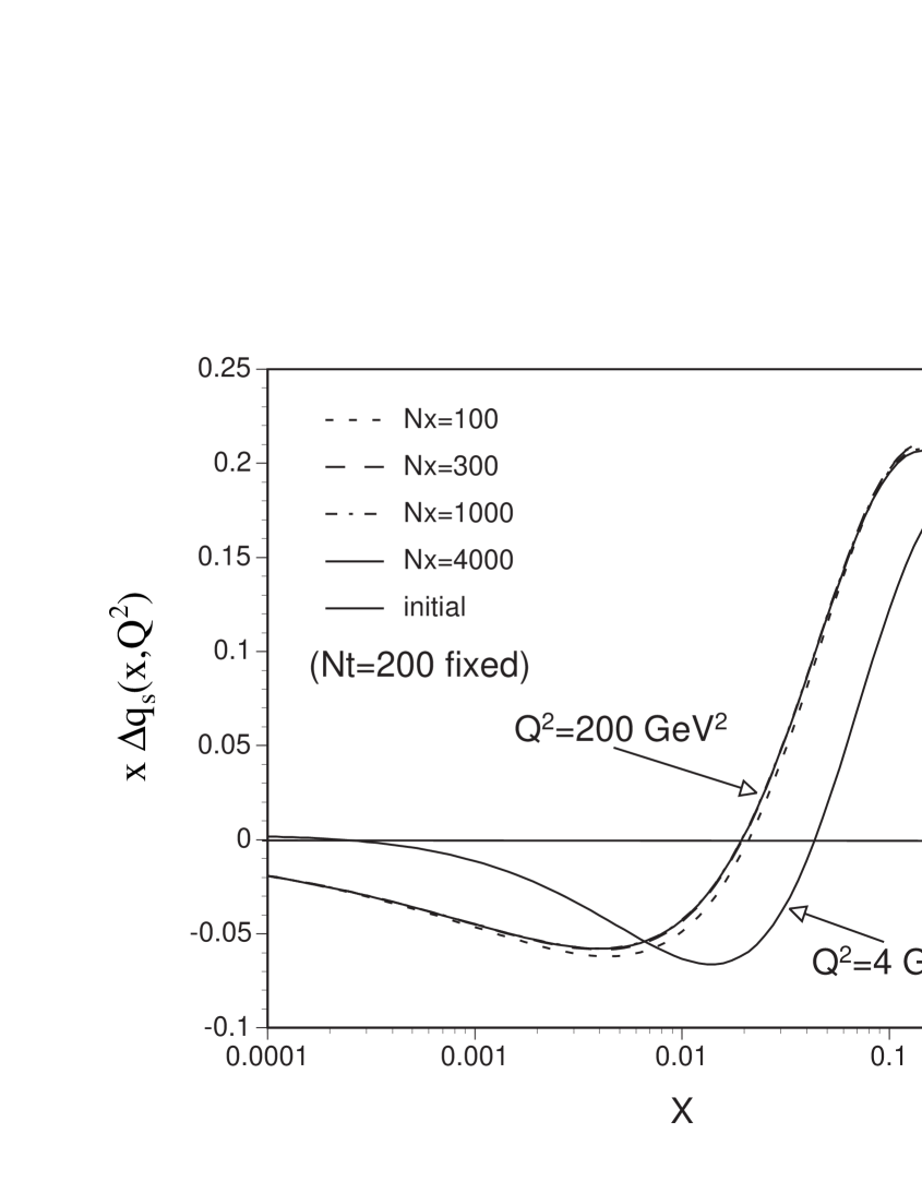
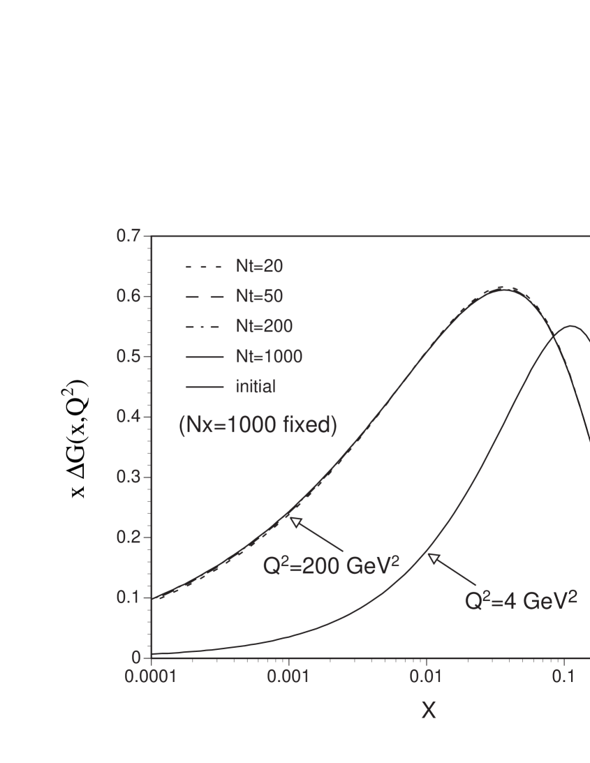
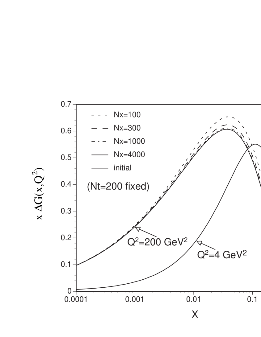
Next, the step $N_{x}$ is varied with fixed $N_{t}$=200 in Fig. 2. $N_{x}$=100, 300, 1000, and 4000 are taken. Even in the 300 steps, we obtain rather accurate results. The evolution results become slightly worse in the gluon case as shown in Figs. 3 and 4. Defining the evolution accuracy by $|\,[\Delta p(N_{x},N_{t})-\Delta p(N_{x}=4000,N_{t}=1000)]/\Delta p(N_{x}=4000,N_{t}=1000)\,|$, we find that the accuracy is better than 1% in the region $10^{-5}<x<0.8$ with $N_{x}=1000$ and $N_{t}=200$. However, it takes rather a significant amount of running CPU time. It is typically seven minutes on the AlphaServer 2100 4/200 in a nonsinglet case and sixty minutes in a singlet case. Our program is good enough for a single evolution calculation, but it is not efficient enough for repeated use. We will work on a much faster program in future.

We also check our results with other publications. First, the evolution in Ref. [7] from $Q^{2}$=4 GeV² to $Q^{2}$=50 GeV² are compared with our results. The structure functions $xg_{1}^{p}$ and $xg_{1}^{n}$ at $Q^{2}$=50 GeV² agree well with our evolved ones. Second, the evolution in Ref. [10] is compared with ours. The GS-A input distributions are used. They are evolved to the ones at $Q^{2}$=10 GeV² with $\Lambda$=239 MeV and are also devolved to the ones at $Q^{2}$=2 GeV². The singlet distribution $\Delta q_{s}$ and the gluon distribution $\Delta g$ are compared. We find that they agree well with our evolution results. From these studies on our results in comparison with others and from repeated checks on our evolution program, we find that the program BFP1 is reliable. We should mention that there is another work [11] on the NLO evolution in addition to Refs. [7] and [10].

6.2 Calculation of $g_{1}$ from output data

We do not supply the BFP1 program so that the structure function $g_{1}$ is obtained directly in the output file. It is because $g_{1}$ depends on the number of flavor and because the precise evolution should be described by setting flavor thresholds. We ask the reader to set up these points by oneself with our program. Actual evolution results for $g_{1}$ are shown in the next subsection, where the following prescription is used for calculating $g_{1}$ from the output data file #11.

First, IOUT=5 or 6 should be chosen so that the evolution of $\Delta q_{i}^{+}(x)$, $\Delta q_{j}^{+}(x)$, $\Delta q_{{}_{S}}(x)$, and $\Delta g(x)$ is calculated by Eqs. (2.12) and (2.13). Furthermore, ITYPE=1 should be chosen for calculating the convolution integrals of these evolved distributions with the coefficient functions in Eq. (2.20). The convolution results are written in the output file #11, and we denote them as $g_{1,d}^{+}(x)$, $g_{1,str}^{+}(x)$, $g_{1_{S}}^{+}(x)$, and $g_{1,g}^{+}(x)$. It goes without saying that the convolution is not necessary in the LO case. The LO $g_{1}$ is calculated directly by Eq. (2.19). Next, the $g_{1}$ for the proton is, for example, calculated by choosing $\Delta d^{+}(x)$ and $\Delta s^{+}(x)$ for the distributions $\Delta q_{i}^{+}(x)$ and $\Delta q_{j}^{+}(x)$:

$$g_{1}^{p}(x,Q^{2}) =\frac{1}{2}\,\sum_{i}^{N_{f}}e_{i}^{2}\,\left[\,g_{1,i}(x,Q^{2})+g_{1,g}(x,Q^{2})\,\right]$$

$$=\frac{1}{18}\,\left[\,4\,g_{1_{S}}^{+}(x,Q^{2})-3\,\{g_{1,d}^{+}(x,Q^{2})+g_{1,str}^{+}(x,Q^{2})\}\,\right]+\frac{1}{2}\,\sum_{i}^{N_{f}}e_{i}^{2}\,g_{1,g}(x,Q^{2})\ ,$$ (6.1)

in the three and four flavor cases. Five and six flavor evolution can be calculated in the similar way with a slightly modified equation.

6.3 Comparisons with experimental data

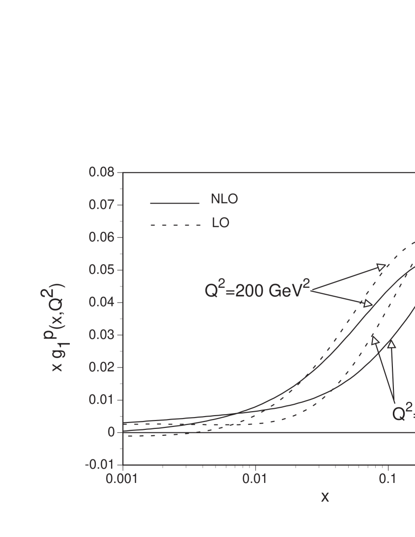
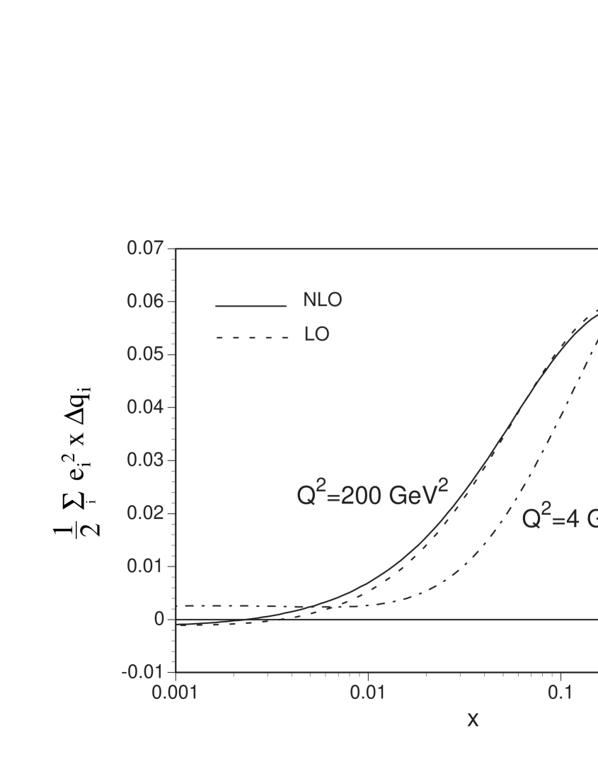
We calculate evolution of the structure function $g_{1}$ and compare its results with experimental data. Using the procedure in the last subsection, we obtain the evolution results for $g_{1}$. The LO and NLO results are shown in Fig. 5. The same GS-A polarized parton distributions are used as the input distributions at $Q^{2}$=4 GeV² in both LO and NLO cases. To be precise, this is not a correct procedure because the GS-A is set up for the NLO $\overline{MS}$ calculation. It should not be used in the LO calculation. Nevertheless, the GS-A distributions are also employed in the LO for finding NLO effects on $g_{1}$. Therefore, the differences between the solid and dashed curves at $Q^{2}$=4 GeV² are purely due to the coefficient functions. Because the coefficient-function contributions are rather large, it is difficult to find the NLO evolution effects from Fig. 5. In order to illustrate the NLO effects from $Q^{2}$=4 GeV² to $Q^{2}$=200 GeV², we show the evolution of the distribution $\sum_{i}e_{i}^{2}\,x\,\Delta q_{i}/2$ in Fig. 6. The same distributions are taken at $Q^{2}$=4 GeV² in the LO and NLO cases. The figure indicates that the NLO effects are positive in the small and large $x$ regions and they are negative in the intermediate region $x\approx 0.2$.

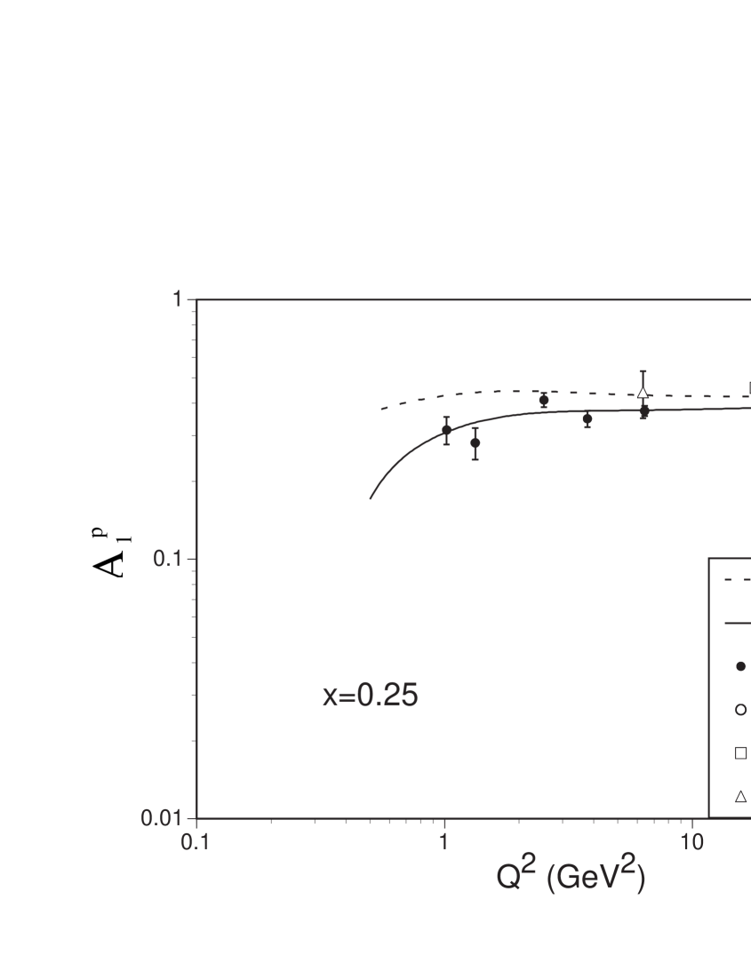
Our evolution results are compared with spin-asymmetry data in Figs. 7, 8, and 9. The SLAC-E130 [12], SLAC-E143 [13], EMC [14], and SMC [15] data are shown in the figures. We comment how the spin asymmetry is calculated theoretically. The asymmetry is given by the structure functions $g_{1}$ and $F_{1}$ as

$$A_{1}\cong\frac{g_{1}(x,Q^{2})}{F_{1}(x,Q^{2})}=g_{1}(x,Q^{2})\,\frac{2\,x\,(1+R)}{F_{2}(x,Q^{2})}\ .$$ (6.2)

The function $R$ is given by $R=(F_{2}-2xF_{1})/(2xF_{1})$, and it could be taken from Ref. [16]. In fitting experimental data for obtaining the optimum unpolarized parton distributions, the $F_{2}$ structure function is used instead of $F_{1}$. Therefore, it is better to calculate the asymmetry with $F_{2}$ if we would like to compare with the experimental data. The MRS-G unpolarized parton distributions [17] are used for calculating $F_{2}$ and the function R in Ref. [16] is used in Eq. (6.2).

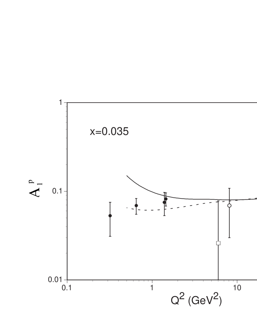
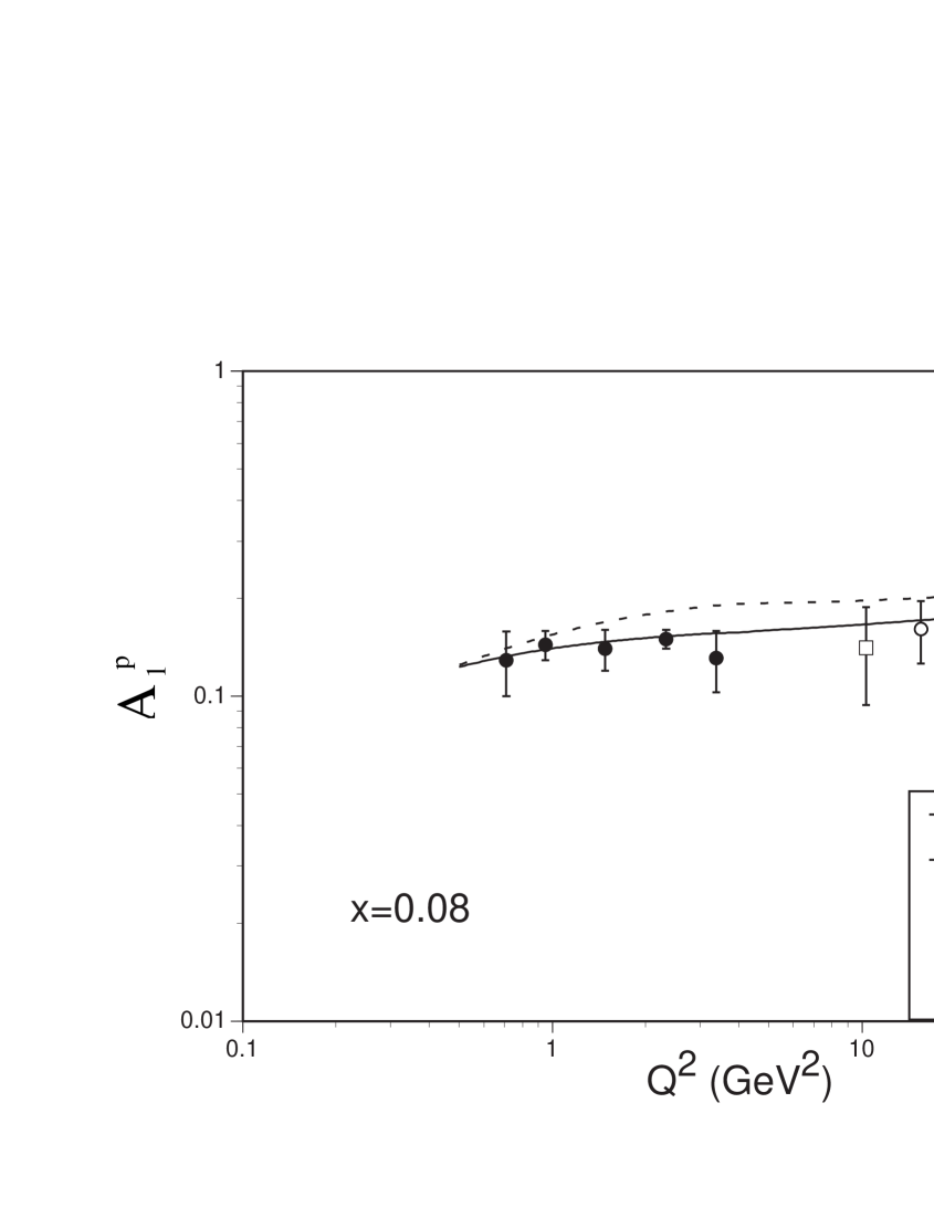
In Fig. 7, our evolution curves at $x$=0.035 are shown with the asymmetry $A_{1}$ data. The dashed and solid curves indicate the LO and NLO evolution results respectively. In the large $Q^{2}$ region, both results are almost the same; however, they differ significantly at small $Q^{2}$ in particular in the region $Q^{2}<\,$2 GeV². The difference is not so large at slightly larger $x$ (=0.08) as shown in Fig. 8. However, the LO values become larger than those of the NLO evolution. In the medium $x$ region ($x$=0.25), the difference becomes larger again at small $Q^{2}$ as shown in in Fig. 9. From these figures, we find that the asymmetry has $Q^{2}$ dependence although it is not large. People used to assume that the asymmetry is independent of $Q^{2}$ by neglecting the $Q^{2}$ evolution difference between $g_{1}$ and $F_{1}$ in analyzing the experimental data. We find clearly that it is not the case. For a precise analysis, the $Q^{2}$ dependence in the asymmetry has to be taken into account. Currently, parametrization studies are in progress [6] by using our program. We expect to obtain NLO fitting results in the near future.

7 Summary

We have investigated numerical solution of the spin-dependent DGLAP equations with or without the NLO corrections. The solution method is so called brute-force method. A FORTRAN program is provided for evolving longitudinally polarized parton distributions including nonsinglet, singlet, each flavor, and gluon distributions. Furthermore, the evolution results could be written in a structure-function form, which is the convolution of the evolved distributions with the coefficient functions. Therefore, the structure function $g_{1}$ could be also calculated from our output data. We checked that typical accuracy is better than 1% with reasonable numbers of steps: $N_{x}$=1000 and $N_{t}$=200. Comparisons with experimental data indicate significant $Q^{2}$ dependence and NLO effects in the region $Q^{2}\approx 1$ GeV². Therefore, the $Q^{2}$ independence assumption, which was used to be employed in analyzing $A_{1}$ experimental data, is not valid. We have to include the $Q^{2}$ evolution differences between $F_{1}$ and $g_{1}$. Our evolution code is very useful for theoretical and experimental researchers in high-energy spin physics.

Appendix A. Splitting functions

First, the constants $\beta_{0}$, $\beta_{1}$ $C_{G}$, $C_{F}$, and $T_{R}$ are given by the number of color ($N_{c}$=3) and the number of flavor ($N_{f}$) as

$$\beta_{0}=\frac{11}{3}C_{G}-\frac{4}{3}T_{R}N_{f}\ ,\ \ \ \ \beta_{1}=\frac{34}{3}C^{2}_{G}-\frac{10}{3}C_{G}N_{f}-2C_{F}N_{f}\ ,$$ (A.1)

$$C_{G}=N_{c}\ ,\ \ \ C_{F}=\frac{N_{c}^{2}-1}{2N_{c}}\ ,\ \ \ T_{R}=\frac{1}{2}\ .$$ (A.2)

Splitting function in the leading order(LO) are

$$\Delta P_{NS}^{(0)}(x) =C_{F}\,\left[\,\frac{2}{(1-x)_{+}}-1-x+\frac{3}{2}\,\delta(1-x)\,\right]\ ,$$

$$\Delta P_{q_{i}^{+}q_{j}^{+}}^{(0)}(x) =\delta_{ij}\,\Delta P_{NS}^{(0)}(x)\ ,$$

$$\Delta P_{q_{i}^{+}g}^{(0)}(x) =2\,T_{R}\,(2x-1)\ ,$$

$$\Delta P_{gq_{i}^{+}}^{(0)}(x) =C_{F}\,(2-x)\ ,$$

$$\Delta P_{gg}^{(0)}(x) =2\,C_{G}\,\left[\,\frac{1}{(1-x)_{+}}-2x+1\,\right]+\frac{\beta_{0}}{2}\,\delta(1-x)\ ,$$ (A.3)

where the $+$ function is defined by

$$\int_{0}^{1}dx\,{\frac{f(x)}{(1-x)_{+}}}\ =\ \int_{0}^{1}dx\,{\frac{f(x)-f(1)}{1-x}}\ .$$ (A.4)

It should be noted that the above integration is defined in the region $0\leq x\leq 1$.

The NLO splitting functions for $\Delta q^{+}_{i}(x)$ and $\Delta g(x)$ are given by [5]

$$\Delta P^{(1)}_{q^{+}_{i}q^{+}_{j}}(x) =\delta_{ij}\,\Delta P^{(1)}_{q^{+},NS}+2\,C_{F}\,T_{R}\,F_{qq}\ ,$$

$$\Delta P^{(1)}_{q^{+}_{i}g}(x) =C_{F}\,T_{R}\,F^{1}_{qg}(x)+C_{G}\,T_{R}\,F^{2}_{qg}(x)\ ,$$

$$\Delta P^{(1)}_{gq^{+}_{i}}(x) =C_{F}\,T_{R}\,N_{f}\,F^{1}_{gq}(x)+C^{2}_{F}\,F^{2}_{gq}(x)+C_{F}\,C_{G}\,F^{3}_{gq}(x)\ ,$$ (A.5)

$$\Delta P^{(1)}_{gg}(x) =-C_{G}\,T_{R}\,N_{f}\,F^{1}_{gg}(x)-C_{F}\,T_{R}\,N_{f}\,F^{2}_{gg}(x)+C^{2}_{G}\,F^{3}_{gg}(x)\ .$$

The splitting functions in the singlet equations (2.12) are expressed as

$$\Delta P_{qq}\otimes\Delta q_{s} =\sum_{i,j}\Delta P_{q^{+}_{i}q^{+}_{j}}\otimes\Delta q_{j}\ ,\ \ \Delta P_{qg}\otimes\Delta g=\sum_{i}\Delta P_{q^{+}_{i}g}\otimes\Delta g\ ,$$

$$\Delta P_{gq}\otimes\Delta q_{s} =\sum_{j}\Delta P_{gq^{+}_{j}}\otimes\Delta q_{j}\ .$$ (A.6)

The splitting function $\Delta P^{(1)}_{q^{\pm},NS}$ is given

$$\Delta P^{(1)}_{q^{\pm},NS}=P^{(1)}_{q^{\mp},NS}\ ,$$ (A.7)

where $P^{(1)}_{q^{\mp},NS}$ are the unpolarized NLO nonsinglet splitting functions. The $\pm$ in these equations indicates “$\Delta q\pm\Delta\bar{q}$ type” distribution $\sum_{i}a_{i}(\Delta q_{i}\pm\Delta\bar{q}_{i})$. The function $\Delta P^{(1)}_{q^{\pm},NS}$ is given by

$$\Delta P^{(1)}_{q^{\pm},NS}(x)= C_{F}^{2}\biggl{\{}P_{F}(x)\mp P_{A}(x)+\delta(1-x)\biggl{[}\frac{3}{8}-\frac{1}{2}\pi^{2}+\zeta(3)-8\widetilde{S}(\infty)\biggr{]}\biggr{\}}$$

$$+\frac{1}{2}C_{F}C_{A}\bigg{\{}P_{G}(x)\pm P_{A}(x)+\delta(1-x)\biggl{[}\frac{17}{12}+\frac{11}{9}\pi^{2}-\zeta(3)+8\widetilde{S}(\infty)\biggr{]}\biggr{\}}$$

$$+C_{F}T_{R}N_{f}\biggl{\{}P_{N_{F}}(x)-\delta(1-x)\biggl{(}\frac{1}{6}+\frac{2}{9}\pi^{2}\biggr{)}\biggr{\}}\ ,$$ (A.8)

where $P_{F}(x)$, $P_{G}(x)$, $P_{N_{F}}(x)$, and $P_{A}(x)$ are given in Ref. [18]

$$P_{F}(x) =-2{\frac{1+x^{2}}{1-x}}\ln x\ln(1-x)-\biggl{(}{\frac{3}{1-x}}+2x\biggr{)}\ln x-\frac{1}{2}(1+x)\ln^{2}x-\!\!5(1-x)\ ,$$

$$P_{G}(x) =\frac{1+x^{2}}{(1-x)_{+}}\bigg{[}\ln^{2}x+\frac{11}{3}\ln x+\frac{67}{9}-\frac{1}{3}\pi^{2}\biggr{]}+2(1+x)\ln x+\frac{40}{3}(1-x)\ ,$$

$$P_{N_{F}}(x) =\frac{2}{3}\Biggl{[}\frac{1+x^{2}}{(1-x)_{+}}\biggl{(}-\ln x-\frac{5}{3}\biggr{)}-2(1-x)\Biggr{]}\ ,$$

$$P_{A}(x) =2\frac{1+x^{2}}{1+x}\int_{x/(1+x)}^{1/(1+x)}\frac{dz}{z}\ln\frac{1-z}{z}+2(1+x)\ln x+4(1-x)\ .$$ (A.9)

The functions $F_{qq}$, $F_{qg}$, $F_{gq}$, and $F_{gg}$ are defined by

$$F_{qq}(x)=(1-x)-(1-3x)\ln x-(1+x)\ln^{2}x\ ,$$ (A.10)

$$F^{1}_{qg}(x)= -22+27x-9\ln x+8(1-x)\ln(1-x)$$

$$+\delta p_{qg}(x)\left[2\ln^{2}(1-x)-4\ln(1-x)\ln x+\ln^{2}x-\frac{2}{3}\pi^{2}\right]\ ,$$

$$F^{2}_{qg}(x)= \,2(12-11x)-8(1-x)\ln(1-x)+2(1+8x)\ln x$$

$$-2\left[\ln^{2}(1-x)-\frac{\pi^{2}}{6}\right]\delta p_{qg}(x)-\left[2S_{2}(x)-3\ln^{2}x\right]\delta p_{qg}(-x)\ ,$$ (A.11)

$$F^{1}_{gq}(x)= -\frac{4}{9}(x+4)-\frac{4}{3}\delta p_{gq}(x)\ln(1-x)\ ,$$

$$F^{2}_{gq}(x)= -\frac{1}{2}-\frac{1}{2}(4-x)\ln x-\delta p_{gq}(-x)\ln(1-x)+\left[-4-\ln^{2}(1-x)+\frac{1}{2}\ln^{2}x\right]\delta p_{gq}(x)\ ,$$

$$F^{3}_{gq}(x)= \,(4-13x)\ln x+\frac{1}{3}(10+x)\ln(1-x)+\frac{1}{9}(41+35x)$$

$$+\frac{1}{2}[-2S_{2}(x)+3\ln^{2}x]\delta p_{gq}(-x)$$

$$+\left[\ln^{2}(1-x)-2\ln(1-x)\ln x-\frac{\pi^{2}}{6}\right]\delta p_{gq}(x)\ ,$$ (A.12)

$$F^{1}_{gg}(x)= \,4(1-x)+\frac{4}{3}(1+x)\ln x+\frac{20}{9}\delta p_{gg}(x)+\frac{4}{3}\delta(1-x)\ ,$$

$$F^{2}_{gg}(x)= \,10(1-x)+2(5-x)\ln x+2(1+x)\ln^{2}x+\delta(1-x)\ ,$$

$$F^{3}_{gg}(x)= \,\frac{1}{3}(29-67x)\ln x-\frac{19}{2}(1-x)+4(1+x)\ln^{2}x-2S_{2}(x)\delta p_{gg}(-x)$$

$$+\left[\frac{67}{9}-4\ln(1-x)\ln x+\ln^{2}x-\frac{\pi^{2}}{3}\right]\delta p_{gg}(x)+\left[3\zeta(3)+\frac{8}{3}\right]\delta(1-x)\ ,$$ (A.13)

where, $\delta p_{qg}\ ,\delta p_{gq}\ ,\delta p_{gg}$ are defined

$$\delta p_{qg}(x) \equiv 2x-1\ ,$$

$$\delta p_{gq}(x) \equiv 2-x\ ,$$ (A.14)

$$\delta p_{gg}(x) \equiv\frac{1}{(1-x)_{+}}-2x+1\ .$$

The $\zeta$ function is defined by $\zeta(k)=\sum_{n=1}^{\infty}\frac{1}{n^{k}}$, and $\zeta(3)$ is given by the numerical value ($\zeta(3)$=1.2020569…). The $S_{2}$ function is expressed in terms of the Spence function $S(x)$

$$S_{2}(x) =\int_{x/(1+x)}^{1/(1+x)}\frac{dz}{z}\ln{\frac{1-z}{z}}$$

$$=S\left({\frac{x}{1+x}}\right)-S\left({\frac{1}{1+x}}\right)-\frac{1}{2}\left[\ln^{2}\frac{1}{1+x}-\ln^{2}\frac{x}{1+x}\right]\ ,$$ (A.15)

where $S(x)$ is defined by

$$S(x)\,=\,\int_{x}^{1}dz\,\frac{\ln z}{1-z}\ .$$ (A.16)

It should be noted that another convention is sometimes used, namely $-S(x)$ may be called the Spence function. It is useful to use a series expansion form for numerical calculations

$$S(x)\,=\,-\,\sum_{k=1}^{\infty}\frac{(1-x)^{k}}{k^{2}}\ .$$ (A.17)

Appendix B. Coefficient functions

The coefficient functions $\Delta C_{q}$ and $\Delta C_{q}$ are [5]

$$\Delta C_{q}(x,\alpha_{s}) =\delta(1-x)+\frac{\alpha_{s}}{2\pi}\,\Delta B_{q}(x)\ ,$$ (B.18)

$$\Delta C_{g}(x,\alpha_{s}) =\frac{\alpha_{s}}{2\pi}\,\Delta B_{g}(x)\ ,$$ (B.19)

where the functions $\Delta B_{q}$ and $\Delta B_{g}$ are

$$\Delta B_{q}(x)= \,C_{F}\Bigg{[}(1+x^{2})\left\{\frac{\ln(1-x)}{1-x}\right\}_{+}-\frac{3}{2}\frac{1}{(1-x)_{+}}-\frac{1+x^{2}}{1-x}\ln x$$

$$+2+x-\left(\frac{9}{2}+\frac{\pi^{2}}{3}\right)\delta(1-x)\Bigg{]}\ ,$$ (B.20)

$$\Delta B_{g}(x)= \,2\,T_{R}\left[(2x-1)\left(\ln\frac{1-x}{x}-1\right)+2(1-x)\right]\ .$$ (B.21)

TEST RUN OUTPUT

IOUT= 3   IREAD= 1   INDIST= 1 IORDER= 2   ITYPE= 2   IMORP= 2
Q02= 4.0000   Q2= 200.000   DLAM= 0.2310   NF= 4
XX= 0.0000000   NX=1000   NT= 200   NSTEP= 50   NXMIN= $-$4

0.000100	-0.019166	0.097380
0.000120	-0.020672	0.105178
0.000145	-0.022276	0.113534
0.000174	-0.023982	0.122478
0.000209	-0.025790	0.132045
0.000251	-0.027703	0.142266
0.000302	-0.029718	0.153174
0.000363	-0.031833	0.164803
0.000437	-0.034043	0.177185
0.000525	-0.036338	0.190351
0.000631	-0.038707	0.204330
0.000759	-0.041130	0.219150
0.000912	-0.043584	0.234833
0.001096	-0.046036	0.251398
0.001318	-0.048444	0.268856
0.001585	-0.050754	0.287209
0.001905	-0.052898	0.306451
0.002291	-0.054790	0.326559
0.002754	-0.056324	0.347493
0.003311	-0.057372	0.369192
0.003981	-0.057777	0.391566
0.004786	-0.057353	0.414496
0.005754	-0.055883	0.437819
0.006918	-0.053115	0.461325
0.008318	-0.048770	0.484750
0.010000	-0.042545	0.507761
0.012023	-0.034126	0.529949
0.014454	-0.023214	0.550821
0.017378	-0.009552	0.569787
0.020893	0.007027	0.586160
0.025119	0.026539	0.599147
0.030200	0.048784	0.607861
0.036308	0.073276	0.611331
0.043652	0.099181	0.608536
0.052481	0.125309	0.598449
0.063096	0.150159	0.580109
0.075858	0.172073	0.552726
0.091201	0.189500	0.515809
0.109648	0.201326	0.469336
0.131826	0.207180	0.413952
0.158489	0.207504	0.351177
0.190546	0.203229	0.283585
0.229087	0.194990	0.214868
0.275423	0.182213	0.149663
0.331131	0.162801	0.092992
0.398107	0.134220	0.049196
0.478630	0.096195	0.020506
0.575440	0.053887	0.005833
0.691831	0.018721	0.000825
0.831764	0.001943	0.000022
1.000000	0.000000	0.000000

Figures

Figure 1: $N_{t}$ dependence of singlet evolution results is shown. The initial distribution is the GS-A at Q²=4 GeV². It is evolved to the one at Q²=200 GeV² by the next-to-leading-order DGLAP evolution equations. $N_{x}$=1000 is fixed and $N_{t}$ is varied ($N_{t}$=20, 50, 200, and 1000). There are dotted, dashed, dot-dashed, and solid curves at $Q^{2}$=200 GeV² for $N_{t}$=20, 50, 200, and 1000 respectively.

      

Figure 2: $N_{x}$ dependence of singlet evolution results is shown. The initial distribution is the same in Fig. 1. $N_{t}$=200 is fixed and $N_{x}$ is varied ($N_{x}$=100, 300, 1000, and 4000). There are dotted, dashed, dot-dashed, and solid curves at $Q^{2}$=200 GeV² for $N_{x}$=100, 300, 1000, and 4000 respectively.

      

Figure 3: $N_{t}$ dependence of gluon evolution results is shown. Notations are the same with those in Fig. 1.

      

Figure 4: $N_{x}$ dependence of gluon evolution results is shown. Notations are the same with those in Fig. 2.

      

Figure 5: $Q^{2}$ evolution results for the proton structure function $g_{1}$ are shown. The solid curves are $xg_{1}$ at $Q^{2}$=4 and 200 GeV² in the NLO case, and the dashed ones are in the LO.

      

Figure 6: $Q^{2}$ evolution results for the distribution $\sum_{i}e_{i}^{2}\,x\,\Delta q_{i}/2$ are shown. The same distributions are assumed at $Q^{2}$=4 GeV² and the evolved distributions are shown by the solid curve in the NLO case and by the dashed one in the LO at 200 GeV².

      

Figure 7: $Q^{2}$ dependence of the spin asymmetry $A_{1}$ for the proton is calculated in the LO and NLO cases. Calculated results at $x=0.035$ are compared with SLAC-143 [13], EMC [14], and SMC [15] experimental data. The solid curve is in the NLO case and the dashed one is in the LO.

      

Figure 8: $Q^{2}$ dependence of the spin asymmetry $A_{1}$ at $x=0.08$. Notations are same with those in Fig. 7.

      

Figure 9: $Q^{2}$ dependence of the spin asymmetry $A_{1}$ at $x=0.25$. Notations are same with those in Fig. 7. The SLAC-E130 data [12] is added.

References

• [1] V. N. Gribov and L. N. Lipatov, Sov. J. Nucl. Phys. 15 (1972) 438 and 675; G. Altarelli and G. Parisi, Nucl. Phys. B 126 (1977) 298; Yu. L. Dokshitzer, Sov. Phys. JETP 46 (1977) 641.
• [2] S. Kumano and J. T. Londergan, Comput. Phys. Commun. 69 (1992) 373; R. Kobayashi, M. Konuma, and S. Kumano, Comput. Phys. Commun. 86 (1995) 264.
• [3] M. Miyama and S. Kumano, Comput. Phys. Commun. 94 (1996) 185.
• [4] W.-K. Tung, private communications.
• [5] R. Mertig and W. L. van Neerven, Z. Phys. C70, 637 (1996); W. Vogelsang, Phys. Rev. D54, 2023 (1996).
• [6] RHIC-SPIN-J parametrization group: Y. Goto, N. Hayashi, M. Hirai, H. Horikawa, S. Kumano, M. Miyama, T. Morii, N. Saito, T.-A. Shibata, E. Taniguchi, and T. Yamanishi, research in progress.
• [7] T. Gehrmann and W. J. Stirling, Phys. Rev. D. 53 (1996) 6100. Other available distributions are found in Ref. [8].
• [8] G. A. Ladinsky, hep-ph/9601287; Parton-distribution-function web sites: http:
//durpdg.dur.ac.uk/HEPDATA/HEPDATA.html, http://www.phys.psu.edu/~~absent\tilde{\ }cteq.
• [9] S. Kumano, preprint-97-97, submitted to Physics Reports.
• [10] T. Weigl and W. Melnitchouk, Nucl. Phys. B465 (1990) 267.
• [11] J. BlΓΌmlein and A. Vogt, pp. 218-221 in Proceedings of the 12th Symposium on High-Energy Spin Physics, edited by C. W. de Jager et al., World Scientific (1997).
• [12] G. Baum et al. (SLAC-E130 collaboration), Phys. Rev. Lett. 51 (1983) 1135.
• [13] K. Abe et al. (SLAC-E143 collaboration), Phys. Lett. B 364 (1995) 61.
• [14] J. Ashman et al. (EMC collaboration), Phys. Lett. B 206 (1988) 364; Nucl. Phys. B 328 (1989) 1.
• [15] D. Adams et al. (SMC collaboration), Phys. Lett. B 329 (1994) 399.
• [16] L. W. Whitlow, S. Rock, A. Bodek, S. Dasu, and E.M. Riordan, Phys. Lett. B 250 (1990) 193.
• [17] A. D. Martin, W. J. Stirling, and R. G. Roberts, Phys. Lett. B 354 (1995) 155.
• [18] G. Curci, W. Furmanski, and R. Petronzio, Nucl. Phys. B 175 (1980) 27.