DYNAMICAL DETERMINATION OF THE TOP QUARK AND HIGGS MASSES AND FERMION MASSES IN THE ANTI-GRAND UNIFICATION MODEL

1 Introduction

On rather general grounds, we expect that all coupling constants become dynamical in quantum gravity due to the non-local effects of baby universes. $\!{}^{{\bf?}}$. We have argued $\!{}^{{\bf?}}$ that the mild form of non-locality in quantum gravity, respecting reparameterisation invariance $\!{}^{{\bf?}}$, leads to the realisation in Nature of the “multiple point criticality principle”. According to this principle, Nature should choose coupling constant values such that the vacuum can exist in degenerate phases, in a very similar way to the stable coexistence of ice, water and vapour (in a thermos flask for example) in a mixture with fixed energy and number of molecules. We apply this principle to the pure Standard Model (SM) with a desert up to the Planck scale, and give a precise dynamical determination of the top quark mass $M_{t}$ and the Higgs particle mass $M_{H}$.

The top quark is the only SM fermion which has a mass of order the electroweak scale and a SM Yukawa coupling of order unity. All of the other fermion masses are suppressed relative to the natural scale of the SM. The Yukawa couplings range over five orders of magnitude, from of order $10^{5}$ for the electron to of order unity for the top quark. It is this fermion mass hierarchy problem that we address in the second half of the talk. We introduce an extension of the SM where such a large range of Yukawa couplings is natural, due to the existence of new approximately conserved chiral gauge quantum numbers which protect the fermions from gaining a mass. This so-called anti-grand unification model $\!{}^{{\bf?}}$ is based on the gauge group $SMG^{3}\otimes U(1)_{f}$, where $SMG=SU(3)\otimes SU(2)\otimes U(1)$. In our model all the elements of the Yukawa matrices (except for one element which leads to the unsuppressed top mass) are suppressed (relative to the assumed natural order 1) by a product of the ratios of the vacuum expectation values (VEVs) of the Higgs fields required to break the extended gauge symmetry to the fundamental (Planck) scale of the theory. In this way we can express very small numbers such as $10^{-5}$ as the product of 5 numbers of order $10^{-1}$.

2 The Ice-Water Analogue

In the analogy of the ice, water and vapour system, the important point for us is that by enforcing fixed values of the extensive quantities, such as energy, the number of moles and the volume, you can very likely come to make such a choice of these values that a mixture has to occur. In that case then the temperature and pressure (i. e. the intensive quantities) take very specific values, namely the values at the triple point. We want to stress that this phenomenon of thus getting specific intensive quantities only happens for first order phase transitions, and it is only likely to happen for rather strongly first order phase transitions. By strongly first order, we here mean that the interval of values for the extensive quantities which do not allow the existence of a single phase is rather large. Because the phase transition between water and ice is first order, one very often finds slush (partially melted snow or ice) in winter at just zero degree celsius. And conversely you may guess with justification that if the temperature happens to be suspiciously close to zero, it is because of the existence of such a mixture: slush. But for a very weakly first order or second order phase transition, the connection with a mixture is not so likely.

In the analogy considered in this paper the coupling constants, such as the Higgs self coupling and the top quark Yukawa coupling, correspond to intensive quantities like temperature and pressure. Now it is well-known that the pure Standard Model, with one loop corrections say, can have two minima in the effective Higgs field potential. If really there were some reason for Nature to require phase coexistence, it would be expected that the “vacua” corresponding to these minima should be able to energetically coexist, which means that they should be degenerate. If the vacuum degeneracy requirement should have a good chance of being relevant, the “phase transition” between the two vacua should be strongly first order. That is to say there should be an appreciable interval of extensive variable values leading to a necessity for the presence of the two phases in the Universe. Such an extensive variable might be e. g. $\int d^{4}x|\phi(x)|^{2}$. If, as we shall assume, Planck units reflect the fundamental physics, it would be natural to interpret this strongly first order transition requirement to mean that, in Planck units, the extensive variable densities $\frac{\int d^{4}x|\phi(x)|^{2}}{\int d^{4}x}$ = $<|\phi|^{2}>$ for the two vacua should differ by a quantity of order unity. Phenomenologically $|\phi|^{2}$ is very small in Planck units for the vacuum in which we live, and hence the other vacuum should have $|\phi|^{2}$ of order unity in Planck units.

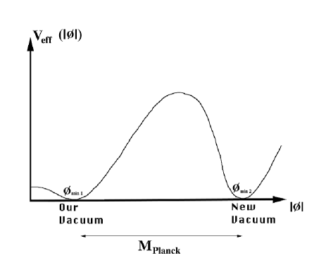
Figure 1: This symbolic graph of the effective potential $V_{\rm{eff}}(\phi)$ for the Standard Model Higgs field illustrates the two assumptions which lead to our prediction of the top quark and Higgs boson masses: 1) Two equally deep minima, 2) achieved for $|\phi|$ values differing, order of magnitudewise, by unity in Planck units.

Thus the application of the multiple point criticality principle to the pure SM leads to our two crucial assumptions:
a) The two minima in the SM effective Higgs potential are degenerate: $V_{\rm{eff}}(\phi_{\rm{min}\;1})=V_{\rm{eff}}(\phi_{\rm{min}\;2})$.
b) The second minimum has a Higgs field squared: $<|\phi_{\rm{min}\;2}|^{2}>={\cal O}(M_{\rm{Planck}}^{2})\sim(10^{19}$ GeV)².
These assumptions are illustrated in Figure 1 and in the next section we show how they lead to precise predictions for $M_{t}$ and $M_{H}$.

3 Calculation of the Higgs and Top Masses

We use the renormalisation group improved effective potential, identifying the renormalisation point with the field strength $\phi$:

$$V_{\rm{eff}}(\phi)\;=\;\frac{1}{2}m_{h}^{2}(\mu=|\phi|)\,|\phi|^{2}\;+\;\frac{1}{8}\lambda(\mu=|\phi|)\,|\phi|^{4}$$ (1)

Now the condition $V_{\rm{eff}}(\phi_{\rm{min}\;1})=V_{\rm{eff}}(\phi_{\rm{min}\;2})$, where one of the minima corresponds to our vacuum with $\phi_{\rm{min}\;1}=246$ GeV, defines (part of) the vacuum stability curve in the $M_{t}-M_{H}$ plane, for $\phi_{\rm{min}\;2}<\Lambda$. Here $\Lambda$ is the physical cut-off scale for the pure SM beyond which new physics enters. We take $\Lambda\simeq M_{\rm{Planck}}\sim 10^{19}$ GeV and the vacuum stability curve for this case is illustrated $\!{}^{{\bf?}}$ in Figure 2

Figure 2: SM vacuum stability curve for $\Lambda=10^{19}$ GeV and $\alpha_{s}=0.124$ (solid line), $\alpha_{s}=0.118$ (upper dashed line), $\alpha_{s}=0.130$ (lower dashed line).

If we now also impose the strong first order transition requirement, $\phi_{\rm{min}\;2}={\cal O}(\rm{M}_{\rm{Planck}})$ we are interested in the situation when $\phi_{\rm{min}\;2}\gg\phi_{\rm{min}\;1}$. In this case the energy density in our vacuum 1 is exceedingly small compared to $\phi^{4}_{\rm{min}\;2}$. Also the $|\phi|^{4}$ term will a priori strongly dominate the $|\phi|^{2}$ term in vacuum 2. So we basically get the vacuum degeneracy condition to mean that, at the vacuum 2 minimum, the effective coefficient $\lambda(\phi_{\rm{min}\;2})$ must be zero with high accuracy. At the same $\phi$-value the derivative of the effective potential $V_{\rm{eff}}(\phi)$ should be zero, because it has a minimum there. In the approximation $V_{\rm{eff}}(\phi)\approx\frac{1}{8}\lambda(\phi)\phi^{4}$ the derivative of $V_{\rm{eff}}(\phi)$ with respect to $\phi$ becomes

$$\frac{dV_{\rm{eff}}(\phi)}{d\phi}|_{\phi_{\rm{min}\;2}}=\frac{1}{2}\lambda(\phi)\phi^{3}+\frac{1}{8}\frac{d\lambda(\phi)}{d\phi}\phi^{4}=\frac{1}{8}\beta_{\lambda}\phi^{3}$$ (2)

and thus at the second minimum the beta-function $\beta_{\lambda}$ vanishes, as well as $\lambda(\phi)$. So we imposed the conditions $\beta_{\lambda}=\lambda=0$ near the Planck scale, $\phi_{\rm{min}\;2}\simeq M_{\rm{Planck}}$. Using the two loop renormalisaion group equations, these two conditions determine a single point on the vacuum stability curve, giving our Standard Model criticality prediction for both the top quark and Higgs boson pole masses $\!{}^{{\bf?}}$:

$$M_{t}=173\pm 5\ \mbox{GeV}\quad M_{H}=135\pm 9\ \mbox{GeV}.$$ (3)

4 The Anti-grand Unification Model

The anti-grand unified gauge group is:

$$G=SMG_{1}\otimes SMG_{2}\otimes SMG_{3}\otimes U(1)_{f}$$ (4)

$$\mbox{where}\quad SMG_{i}=SU(3)_{i}\otimes SU(2)_{i}\otimes U(1)_{i}$$ (5)

The three $SMG_{i}$ groups are broken down to their diagonal subgroup—the usual SM gauge group SMG—and the $U(1)_{f}$ group is totally broken near the Planck scale. As discussed by Holger Nielsen at this conference, the multiple point criticality principle applied to this model successfully predicts the values of the three running SM gauge coupling constants $\!{}^{{\bf?}}$.

We put the SM fermions into this group in an obvious way. We have one generation of fermions coupling to each $SMG_{i}$ in exactly the same way as they would couple to the SMG in the SM. We then choose $U(1)_{f}$ charges with the constraint that there should be no anomalies and no new mass-protected fermions, giving the essentially unique set of charges shown in Table 1. We have labelled the fermions coupling to $SMG_{i}$ by the names of the ‘i’th proto-generation of SM fermions.

Table 1: $U(1)_{f}$ charges of the fermions.

$$\begin{array}[]{|c|c|c|c|c|c|}\hline\cr{\rm Fermion}&Q_{f}&{\rm Fermion}&Q_{f}&{\rm Fermion}&Q_{f}\\ \hline\cr u_{L}&0&c_{L}&0&t_{L}&0\\ \hline\cr u_{R}&0&c_{R}&1&t_{R}&-1\\ \hline\cr d_{R}&0&s_{R}&-1&b_{R}&1\\ \hline\cr e_{L}&0&\mu_{L}&0&\tau_{L}&0\\ \hline\cr e_{R}&0&\mu_{R}&-1&\tau_{R}&1\\ \hline\cr\end{array}$$

Now we must choose appropriate Higgs fields to break $G$ down to the SMG. The quantum numbers of the fermion fields are determined by the theoretical structure of the model (in particular the requirement of anomaly cancellation), but we do have some freedom in the choice of the quantum numbers of the Higgs fields. We choose the Higgs fields so as to get a realistic model of the suppression of fermion masses. In fact we specify the U(1) charges of the Higgs fields and use a natural generalisation of the usual SM charge quantisation rule to determine the non-abelian representations. The Weinberg-Salam Higgs field $\phi_{WS}$ takes highly non-trivial quantum numbers under $G$. In this way we determine an order of magnitude representation of the Yukawa coupling matrices, in terms of three Higgs field VEVs; W, T and $\xi$ measured in Planck units. Since we only use the abelian charges, the same results can be obtained in an anomaly free $SMG\otimes U(1)^{3}$ model.

5 Mass Matrices

The fermion mass matrices are expressed in terms of Yukawa matrices and $<\phi_{WS}>=246$ GeV by: $M_{f}=Y_{f}<\phi_{WS}>/\sqrt{2}$. Our model $\!{}^{{\bf?}}$ gives the following order of magnitude Yukawa matrices at the Planck scale, where unknown complex coefficients of $\cal O$(1) in the matrix elements have been ignored.

$$Y_{u} \simeq \left(\begin{array}[]{ccc}WT^{2}\xi^{2}&WT^{2}\xi&W^{2}T\xi\\ WT^{2}\xi^{3}&WT^{2}&W^{2}T\\ \xi^{3}&1&WT\end{array}\right)$$ (9)

$$Y_{d} \simeq \left(\begin{array}[]{ccc}WT^{2}\xi^{2}&WT^{2}\xi&T^{3}\xi\\ WT^{2}\xi&WT^{2}&T^{3}\\ W^{2}T^{4}\xi&W^{2}T^{4}&WT\end{array}\right)$$ (13)

$$Y_{l} \simeq \left(\begin{array}[]{ccc}WT^{2}\xi^{2}&WT^{2}\xi^{3}&WT^{4}\xi\\ WT^{2}\xi^{5}&WT^{2}&WT^{4}\xi^{2}\\ WT^{5}\xi^{3}&W^{2}T^{4}&WT\end{array}\right)$$ (17)

We note that these mass matrices are not symmetric but they do have some important features. The diagonal elements in all 3 mass matrices are the same, giving the SU(5)-like results $m_{b}\approx m_{\tau}$ and $m_{s}\approx m_{\mu}$, but the off-diagonal elements dominate $Y_{u}$ making $m_{t}$ and $m_{c}$ respectively larger. The diagonal and off-diagonal contributions to the lowest eigenvalue of $Y_{d}$ are approximately equal, giving $m_{d}\geq m_{u}\approx m_{e}$. A three parameter order of magnitude fit with W = 0.158, T = 0.081 and $\xi$ = 0.099 successfully reproduces the observed masses and mixing angles within a factor of two—see Table 2.

Table 2: Best fit to experimental data. All masses are running masses at 1 GeV except the top quark mass which is the pole mass.

$$\begin{array}[]{|c|c|c|}\hline\cr&{\rm Fitted}&{\rm Experimental}\\ \hline\cr m_{u}&3.8{\rm\;MeV}&4{\rm\;MeV}\\ \hline\cr m_{d}&7.4{\rm\;MeV}&9{\rm\;MeV}\\ \hline\cr m_{e}&1.0{\rm\;MeV}&0.5{\rm\;MeV}\\ \hline\cr m_{c}&0.83{\rm\;GeV}&1.4{\rm\;GeV}\\ \hline\cr m_{s}&415{\rm\;MeV}&200{\rm\;MeV}\\ \hline\cr m_{\mu}&103{\rm\;MeV}&105{\rm\;MeV}\\ \hline\cr M_{t}&187{\rm\;GeV}&180{\rm\;GeV}\\ \hline\cr m_{b}&7.6{\rm\;GeV}&6.3{\rm\;GeV}\\ \hline\cr m_{\tau}&1.32{\rm\;GeV}&1.78{\rm\;GeV}\\ \hline\cr V_{us}&0.18&0.22\\ \hline\cr V_{cb}&0.029&0.041\\ \hline\cr V_{ub}&0.0030&0.002-0.005\\ \hline\cr\end{array}$$

6 Conclusion

Our determination of the pole masses, $(M_{t},M_{H})=(173\pm 5,135\pm 9)$ GeV follows from 3 assumptions:
1. The pure SM is valid, without any supersymmetry, up to the Planck scale.
2. The SM Higgs potential $V_{\rm{eff}}$ has 2 degenerate minima.
3. There is a strong first order phase transition, requiring $\phi_{\rm{min}\;2}\simeq M_{\rm{Planck}}$.
The coexistence of these 2 vacuum phases in spacetime suggests a mild breakdown of locality as in baby universe theory.

The anti-grand unified $SMG^{3}\otimes U(1)_{f}$ model, or the effective $SMG\otimes U(1)^{3}$ model, successfully fits 9 fermion mases and 3 mixing angles in terms of 3 Higgs VEVs.

References

References

-
[1]
S.W. Hawking, Phys. Rev. D 37, 904 (1988);
S. Coleman, Nucl. Phys. B 307, 867 (1988) Nucl. Phys. B 310, 643 (1988);
W. Fischler, I. Klebanov, J. Polchinski and L. Susskind, Nucl. Phys. B 327, 157 (1989). - [2] C.D. Froggatt and H.B. Nielsen in Proceedings of the 5th Hellenic School and Workshops on Elementary Particle Physics, 1995, ed. G. Koutsoumbas and N. Tracas (World Scientific, to be published), hep-ph 9607375.
- [3] C.D. Froggatt and H.B. Nielsen, Origin of Symmetries (World Scientific, Singapore, 1991).
- [4] D.L. Bennett, H.B. Nielsen and I. Picek, Phys. Lett. B 208, 275 (1988).
- [5] J.A. Casas, J.R. Espinosa and M. Quiros, Phys. Lett. B 342, 171 (1995).
- [6] C.D. Froggatt and H.B. Nielsen, Phys. Lett. B 368, 96 (1996).
- [7] C.D. Froggatt, H.B. Nielsen and D.J. Smith, Phys. Lett. B , (to be published), hep-ph 9607250.