ICRR-Report-393-97-16 UT-779 hep-ph/9707203
$CP$- and $T$-Violation Effects in Long Baseline Neutrino Oscillation Experiments

Abstract

We examine how large $CP$- and $T$-violation effects are allowed in long baseline neutrino experiments with three generations of neutrinos, considering both the solar neutrino deficit and the atmospheric neutrino anomaly. We considerd two cases: When we attribute only the atmospheric neutrino anomaly to neutrino oscillation and assume the constant transition probability of $\nu_{\rm e}$ to explain the solar neutrino deficit, we may have large $CP$-violation effect. When we attribute both the atmospheric neutrino anomaly and the solar neutrino deficit to neutrino oscillation, we can see sizable $T$- violation effects. In this case, however, we cannot ignore the matter effect and we will not see the pure $CP$- violation effect. We also show simple methods how to separate pure $CP$ violating effect from the matter effect. We give compact formulae for neutrino oscillation probabilities assuming one of the three neutrino masses (presumably $\nu_{\tau}$ mass) to be much larger than the other masses and the effective mass due to matter effect. Two methods are shown: One is to observe envelopes of the curves of oscillation probabilities as functions of neutrino energy; a merit of this method is that only a single detector is enough to determine the presence of $CP$ violation. The other is to compare experiments with at least two different baseline lengths; this has a merit that it needs only narrow energy range of oscillation data.

1 Introduction

The $CP$ and $T$ violation is a fundamental and important problem of the particle physics and cosmology. The $CP$ violation has been observed only in the hadron sector, and it is very hard for us to understand where the $CP$ violation originates from. If we observe $CP$ violation in the lepton sector through the neutrino oscillation experiments, we will be given an invaluable key to study the origin of $CP$ violation and to go beyond the Standard Model.

The neutrino oscillation search is a powerful experiment which can examine masses and/or mixing angles of the neutrinos. The several underground experiments, in fact, have shown lack of the solar neutrinos[1, 2, 3, 4] and anomaly in the atmospheric neutrinos[5, 6, 7], strongly indicating the neutrino oscillation[10, 11, 12]. The solar neutrino deficit implies $10^{-5}\sim 10^{-4}\;{\rm eV^{2}}$ as a difference of the masses squared ($\delta m^{2}$), while the atmospheric neutrino anomaly suggests $\delta m^{2}$ around $10^{-3}\sim 10^{-2}{\rm eV^{2}}$[10, 11, 12].

The latter encourages us to make long baseline neutrino oscillation experiments. Recently such experiments are planned and will be operated in the near future[13, 14]. It is now desirable to examine whether there is a chance to observe not only the neutrino oscillation but also the $CP$ or $T$ violation by long baseline experiments[15, 16, 17, 18, 19, 20].

In this paper we review our papers[16, 17, 18] to show how large violation effects of $CP$ and $T$ we may see in long baseline neutrino experiments with three generations of neutrinos, considering both the solar neutrino deficit and the atmospheric neutrino anomaly.

If we are to attribute both solar neutrino deficit and atmospheric neutrino anomaly to neutrino oscillation, it is natural to consider that one of $\delta m^{2}$’s is in the range ${\cal O}(10^{-5}\sim 10^{-4}\;{\rm eV^{2}})$ and the other is in ${\cal O}(10^{-3}\sim 10^{-2}\;{\rm eV^{2}})$. Recently, however, Acker and Pakvasa[21] has argued that it is possible to explain both experiments by only one $\delta m^{2}$ scale around ${\cal O}(10^{-3}\sim 10^{-2}\;{\rm eV^{2}})$. In the former case we cannot ignore the matter effect[22] and will not see pure $CP$ violating effect; pure $CP$ violating effect must be separated from the matter effect. On the other hand, almost pure $CP$ violating effect can be seen in the latter case.

In sec.2 we briefly review $CP$ and $T$ violation in neutrino oscillation. We then consider how large $T$ and $CP$ violating effects can be. The case where both $\delta m^{2}$’s are ${\cal O}(10^{-2}\;{\rm eV^{2}})$ are considered in sec.3. Sec.4 treats the “disparate” case, where the two $\delta m^{2}$’s are ${\cal O}(10^{-2}\;{\rm eV^{2}})$ and ${\cal O}(10^{-4}\;{\rm eV^{2}})$. In sec.5 we summarize our work and give discussions.

2 Formulation of $CP$ and $T$ Violation in Neutrino Oscillation

Let us briefly review $CP$ and $T$ violation in neutrino oscillation [23, 24, 25] to clarify our notation.

We assume three generations of neutrinos which have mass eigenvalues $m_{i}(i=1,2,3)$ and mixing matrix $U$ relating the flavor eigenstates $\nu_{\alpha}(\alpha={\rm e},\mu,\tau)$ and the mass eigenstates in the vacuum $\nu\,^{\prime}_{i}(i=1,2,3)$ as

$$\nu_{\alpha}=U_{\alpha i}\nu\,^{\prime}_{i}.$$ (1)

We parameterize $U$[26, 27, 28] as

$$U={\rm e}^{{\rm i}\psi\lambda_{7}}\Gamma{\rm e}^{{\rm i}\phi\lambda_{5}}{\rm e}^{{\rm i}\omega\lambda_{2}}$$ (14)

$$= \left(\begin{array}[]{ccc}1&0&0\\ 0&c_{\psi}&s_{\psi}\\ 0&-s_{\psi}&c_{\psi}\end{array}\right)\left(\begin{array}[]{ccc}1&0&0\\ 0&1&0\\ 0&0&{\rm e}^{{\rm i}\delta}\end{array}\right)\left(\begin{array}[]{ccc}c_{\phi}&0&s_{\phi}\\ 0&1&0\\ -s_{\phi}&0&c_{\phi}\end{array}\right)\left(\begin{array}[]{ccc}c_{\omega}&s_{\omega}&0\\ -s_{\omega}&c_{\omega}&0\\ 0&0&1\end{array}\right)$$

$$= \left(\begin{array}[]{ccc}c_{\phi}c_{\omega}&c_{\phi}s_{\omega}&s_{\phi}\\ -c_{\psi}s_{\omega}-s_{\psi}s_{\phi}c_{\omega}{\rm e}^{{\rm i}\delta}&c_{\psi}c_{\omega}-s_{\psi}s_{\phi}s_{\omega}{\rm e}^{{\rm i}\delta}&s_{\psi}c_{\phi}{\rm e}^{{\rm i}\delta}\\ s_{\psi}s_{\omega}-c_{\psi}s_{\phi}c_{\omega}{\rm e}^{{\rm i}\delta}&-s_{\psi}c_{\omega}-c_{\psi}s_{\phi}s_{\omega}{\rm e}^{{\rm i}\delta}&c_{\psi}c_{\phi}{\rm e}^{{\rm i}\delta}\end{array}\right),$$ (18)

where $c_{\psi}=\cos\psi,s_{\phi}=\sin\phi$, etc.

The evolution equation for the flavor eigenstate vector in the vacuum is

$${\rm i}\frac{{\rm d}\nu}{{\rm d}x} = -U{\rm diag}(p_{1},p_{2},p_{3})U^{\dagger}\nu$$ (19)

$$\simeq \left\{-p_{1}+\frac{1}{2E}U{\rm diag}(0,\delta m^{2}_{21},\delta m^{2}_{31})U^{\dagger}\right\}\nu,$$

where $p_{i}$’s are the momenta, $E$ is the energy and $\delta m^{2}_{ij}=m^{2}_{i}-m^{2}_{j}$. Neglecting the term $p_{1}$ which gives an irrelevant overall phase, we have

$${\rm i}\frac{{\rm d}\nu}{{\rm d}x}=\frac{1}{2E}U{\rm diag}(0,\delta m^{2}_{21},\delta m^{2}_{31})U^{\dagger}\nu.$$ (20)

Similarly the evolution equation in matter is expressed as

$${\rm i}\frac{{\rm d}\nu}{{\rm d}x}=H\nu,$$ (21)

where

$$H\equiv\frac{1}{2E}\tilde{U}{\rm diag}(\tilde{m}^{2}_{1},\tilde{m}^{2}_{2},\tilde{m}^{2}_{3})\tilde{U}^{\dagger},$$ (22)

with a unitary mixing matrix $\tilde{U}$ and the effective mass squared $\tilde{m}^{2}_{i}$’s $(i=1,2,3)$. (Tilde indicates quantities in the matter in the following). The matrix $\tilde{U}$ and the masses $\tilde{m}_{i}$’s are determined by[29, 30]

$$\tilde{U}\left(\begin{array}[]{ccc}\tilde{m}^{2}_{1}&&\\ &\tilde{m}^{2}_{2}&\\ &&\tilde{m}^{2}_{3}\end{array}\right)\tilde{U}^{\dagger}=U\left(\begin{array}[]{ccc}0&&\\ &\delta m^{2}_{21}&\\ &&\delta m^{2}_{31}\end{array}\right)U^{\dagger}+\left(\begin{array}[]{ccc}a&&\\ &0&\\ &&0\end{array}\right).$$ (23)

Here

$$a \equiv 2\sqrt{2}G_{\rm F}n_{\rm e}E$$ (24)

$$= 7.56\times 10^{-5}{\rm eV^{2}}\frac{\rho}{\rm g\,cm^{-3}}\frac{E}{\rm GeV},$$

where $n_{\rm e}$ is the electron density and $\rho$ is the matter density. The solution of eq.(21) is then

$$\nu(x)=S(x)\nu(0)$$ (25)

with

$$S\equiv{\rm T\,e}^{-{\rm i}\int_{0}^{x}{\rm d}sH(s)}$$ (26)

(T being the symbol for time ordering), giving the oscillation probability for $\nu_{\alpha}\rightarrow\nu_{\beta}(\alpha,\beta={\rm e},\mu,\tau)$ at distance $L$ as

$$P(\nu_{\alpha}\rightarrow\nu_{\beta};E,L) = \left|S_{\beta\alpha}(L)\right|^{2}.$$ (27)

The oscillation probability for the antineutrinos $P(\bar{\nu}_{\alpha}\rightarrow\bar{\nu}_{\beta})$ is obtained by replacing $a\rightarrow-a$ and $U\rightarrow U^{\ast}({\rm i.e.\,}\delta\rightarrow-\delta)$ in eq.(27).

We assume in the following that the matter density is independent of space and time for simplicity. In this case we have

$$S(x)={\rm e}^{-{\rm i}Hx}$$ (28)

and

$$P(\nu_{\alpha}\rightarrow\nu_{\beta};E,L) = \left|\sum_{i,j}\tilde{U}_{\beta i}\left({\rm e}^{-{\rm i}\frac{L}{2E}{\rm diag}(0,\delta\tilde{m}_{21}^{2},\delta\tilde{m}_{31}^{2})}\right)_{ij}\tilde{U}^{\ast}_{\alpha j}\right|^{2}$$ (29)

$$= \sum_{i,j}\tilde{U}_{\beta i}\tilde{U}^{\ast}_{\beta j}\tilde{U}^{\ast}_{\alpha i}\tilde{U}_{\alpha j}{\rm e}^{-{\rm i}\frac{\delta\tilde{m}^{2}_{ij}L}{2E}},$$ (30)

where $\delta\tilde{m}^{2}_{ij}\equiv\tilde{m}^{2}_{i}-\tilde{m}^{2}_{j}$.

The $T$ violation gives the difference between the transition probability of $\nu_{\alpha}\rightarrow\nu_{\beta}$ and that of $\nu_{\beta}\rightarrow\nu_{\alpha}$[31]:

$$P(\nu_{\alpha}\rightarrow\nu_{\beta};E,L)-P(\nu_{\beta}\rightarrow\nu_{\alpha};E,L)$$ (31)

$$= -4({\rm Im}\;\tilde{U}_{\beta 1}\tilde{U}^{\ast}_{\beta 2}\tilde{U}^{\ast}_{\alpha 1}\tilde{U}_{\alpha 2})(\sin\Delta_{21}+\sin\Delta_{32}+\sin\Delta_{13})$$

$$\equiv 4Jf,$$ (32)

where

$$\Delta_{ij} \equiv \frac{\delta\tilde{m}_{ij}^{2}L}{2E}=2.54\frac{(\delta\tilde{m}_{ij}^{2}/10^{-2}{\rm eV}^{2})(L/100{\rm km})}{(E/{\rm GeV})},$$ (33)

$$J \equiv -{\rm Im}\;\tilde{U}_{\beta 1}\tilde{U}^{\ast}_{\beta 2}\tilde{U}^{\ast}_{\alpha 1}\tilde{U}_{\alpha 2},$$ (34)

$$f \equiv \sin\Delta_{21}+\sin\Delta_{32}+\sin\Delta_{13}$$ (35)

$$= -4\sin\frac{\Delta_{21}}{2}\sin\frac{\Delta_{32}}{2}\sin\frac{\Delta_{13}}{2}.$$ (36)

The unitarity of $U$ gives

$$J=\pm\sin\tilde{\delta}\cos^{2}\tilde{\phi}\sin\tilde{\phi}\cos\tilde{\psi}\sin\tilde{\psi}\cos\tilde{\omega}\sin\tilde{\omega}$$ (37)

with the sign $+$ ($-$) for $\alpha,\beta$ in cyclic (anti-cyclic) order ($+$ for $(\alpha,\beta)=(e,\mu),(\mu,\tau)$ or $(\tau,e)$). In the following we assume the cyclic order for ($\alpha$, $\beta$) for simplicity.

There are bounds for $J$ and $f$. $J$ satisfies

$$|J|\leq\frac{1}{6\sqrt{3}},$$ (38)

where the equality holds for $|\sin\tilde{\omega}|=1/\sqrt{2},|\sin\tilde{\psi}|=1/\sqrt{2},|\sin\tilde{\phi}|=1/\sqrt{3}$ and $|\sin\tilde{\delta}|=1$. On the other hand, $f$ satisfies[32]

$$|f|\leq\frac{3\sqrt{3}}{2},$$ (39)

where the equality holds for $\Delta_{21}\equiv\Delta_{32}\equiv 2\pi/3$ (mod $2\pi$).

In the vacuum the $CPT$ theorem gives the relation between the transition probability of anti-neutrino and that of neutrino,

$$P(\bar{\nu}_{\alpha}\rightarrow\bar{\nu}_{\beta};E,L)=P(\nu_{\beta}\rightarrow\nu_{\alpha};E,L),$$ (40)

which relates $CP$ violation to $T$ violation:

$$P(\nu_{\alpha}\rightarrow\nu_{\beta};E,L)-P(\bar{\nu}_{\alpha}\rightarrow\bar{\nu}_{\beta};E,L)$$ (41)

$$= P(\nu_{\alpha}\rightarrow\nu_{\beta};E,L)-P(\nu_{\beta}\rightarrow\nu_{\alpha};E,L).$$

3 Cases of Comparable Mass Differences

Recently Acker and Pakvasa[21] argued the possibility of explaining both solar neutrino experiments and atmospheric neutrino experiments by one mass scale, $\delta m^{2}\sim{\cal O}(10^{-3}\sim 10^{-2}\;{\rm eV^{2}}).$ We first examine this “comparable mass differences” case.

We use a parameter set $(\delta m^{2}_{21},\delta m^{2}_{31})=(3.8,1.4)\times 10^{-2}$eV², $(\omega,\phi,\psi)=(19^{\circ},43^{\circ},41^{\circ})$ with arbitrary $\delta$, derived by Yasuda[12] through the analysis of the atmospheric neutrino anomaly. We need not distinguish $T$ violation and $CP$ violation in this mass region since the matter effect is negligibly small. Equation (41) is hence available.

Using eqs.(32), (37) and (41), this parameter set gives the $CP$-violation effect

$$P(\nu_{\alpha}\rightarrow\nu_{\beta})-P(\bar{\nu}_{\alpha}\rightarrow\bar{\nu}_{\beta})=0.22f(y)\sin\delta,$$ (42)

where

$$f(y)=(\sin 3.8y+\sin 2.4y-\sin 1.4y),$$ (43)

and

$$y=2.5{(L/100{\rm km})\over(E/{\rm GeV})}.$$ (44)

Figure 1: Graph of $f(y)$ of eq.(43). There are high peaks (positive or negative) at $y=0.42,1.4,3.6,4.6\cdots$. Values of $f(y)$ at peaks averaged over energy spread of 10% $\sim$ 20% are $\left<f(0.42)\right>=1.3\sim 1.3,\left<f(1.4)\right>=-1.9\sim-1.8,\left<f(3.6)\right>=2.2\sim 1.4,\left<f(4.6)\right>=-1.5\sim-0.40\cdots$.

Figure 1 shows the oscillatory part $f(y)$. $f(y)$ has many peaks showing the possibility to observe the large $CP$-violation effect. For example, we may see very large difference between the transition probabilities, $\left<P(\nu_{\alpha}\rightarrow\nu_{\beta})-P(\bar{\nu}_{\alpha}\rightarrow\bar{\nu}_{\beta})\right>_{20\%}\sim 0.4\sin\delta$ for $L=250$ km (for KEK/Super-Kamiokande experiment) and $E\sim$ 4.5 GeV corresponding to $y\sim 1.4$. Hence it will be possible to detect $CP$-violation effect if we have large $\sin\delta$.

In general atmospheric neutrino anomaly indicates large mixing angles. We may see a large $CP$-violation effect when we have comparable mass differences. In this respect we note that the long baseline experiments are urgently desirable.

4 Cases of Disparate Mass Differences

Both solar neutrino deficit and atmospheric neutrino anomaly are naturally explained by introducing two mass scales. Solar neutrino experiments suggest a mass difference of ${\cal O}(10^{-5}\sim 10^{-4}\;{\rm eV^{2}})$, while atmospheric neutrino measurements imply ${\cal O}(10^{-3}\sim 10^{-2}\;{\rm eV^{2}})$. Here we consider this “disparate mass difference” case. We see in this case that matter effect given by eq.(24) is the same order of magnitude as the smaller mass scale. Hence we cannot ignore matter effect.

4.1 Transition Probabilities in Presence of Matter

Let us derive simple expressions of oscillation probabilities assuming $a,\delta m^{2}_{21}\ll\delta m^{2}_{31}$. Decomposing $H=H_{0}+H_{1}$ with

$$H_{0}=\frac{1}{2E}U\left(\begin{array}[]{ccc}0&&\\ &0&\\ &&\delta m^{2}_{31}\end{array}\right)U^{\dagger}\\$$ (45)

and

$$H_{1}=\frac{1}{2E}\left\{U\left(\begin{array}[]{ccc}0&&\\ &\delta m^{2}_{21}&\\ &&0\end{array}\right)U^{\dagger}+\left(\begin{array}[]{ccc}a&&\\ &0&\\ &&0\end{array}\right)\right\},$$ (46)

we treat $H_{1}$ as a perturbation and calculate eq.(28) up to the first order in $a$ and $\delta m^{2}_{21}$. Defining $\Omega(x)$ and $H_{1}(x)$ as

$$\Omega(x)={\rm e}^{{\rm i}H_{0}x}S(x)$$ (47)

and

$$H_{1}(x)={\rm e}^{{\rm i}H_{0}x}H_{1}{\rm e}^{-{\rm i}H_{0}x},$$ (48)

we have

$${\rm i}\frac{{\rm d}\Omega}{{\rm d}x}=H_{1}(x)\Omega(x)$$ (49)

and

$$\Omega(0)=1,$$ (50)

which give the solution

$$\Omega(x) = {\rm T\,e}^{-{\rm i}\int_{0}^{x}{\rm d}sH_{1}(s)}$$ (51)

$$\simeq 1-{\rm i}\int_{0}^{x}{\rm d}sH_{1}(s).$$

We note the approximation (51) requires

$$\frac{ax}{2E}\ll 1\quad{\rm and}\quad\frac{\delta m^{2}_{21}x}{2E}\ll 1.$$ (52)

The equations (47) and (51) give

$$S(x)\simeq{\rm e}^{-{\rm i}H_{0}x}+{\rm e}^{-{\rm i}H_{0}x}(-{\rm i})\int_{0}^{x}{\rm d}sH_{1}(s).$$ (53)

We then obtain the oscillation probabilities $P(\nu_{\mu}\rightarrow\nu_{\rm e})$, $P(\nu_{\mu}\rightarrow\nu_{\mu})$ and $P(\nu_{\mu}\rightarrow\nu_{\tau})$ in the lowest order approximation as

$$P(\nu_{\mu}\rightarrow\nu_{\rm e};L)=4\sin^{2}\frac{\delta m^{2}_{31}L}{4E}c_{\phi}^{2}s_{\phi}^{2}s_{\psi}^{2}\left\{1+\frac{a}{\delta m^{2}_{31}}\cdot 2(1-2s_{\phi}^{2})\right\}$$ (54)

$$+ 2\frac{\delta m^{2}_{31}L}{2E}\sin\frac{\delta m^{2}_{31}L}{2E}c_{\phi}^{2}s_{\phi}s_{\psi}\left\{-\frac{a}{\delta m^{2}_{31}}s_{\phi}s_{\psi}(1-2s_{\phi}^{2})+\frac{\delta m^{2}_{21}}{\delta m^{2}_{31}}s_{\omega}(-s_{\phi}s_{\psi}s_{\omega}+c_{\delta}c_{\psi}c_{\omega})\right\}$$

$$- 4\frac{\delta m^{2}_{21}L}{2E}\sin^{2}\frac{\delta m^{2}_{31}L}{4E}s_{\delta}c_{\phi}^{2}s_{\phi}c_{\psi}s_{\psi}c_{\omega}s_{\omega},$$

$$P(\nu_{\mu}\rightarrow\nu_{\mu}) = 1+4\sin^{2}\frac{\delta m_{31}^{2}L}{4E}c_{\phi}^{2}s_{\psi}^{2}\left\{(c_{\phi}^{2}s_{\psi}^{2}-1)+\frac{a}{\delta m_{31}^{2}}\cdot 2s_{\phi}^{2}(1-2c_{\phi}^{2}s_{\psi}^{2})\right\}$$ (55)

$$+ 2\frac{\delta m_{31}^{2}L}{2E}\sin\frac{\delta m_{31}^{2}L}{2E}c_{\phi}^{2}s_{\psi}^{2}\left\{\frac{a}{\delta m_{31}^{2}}s_{\phi}^{2}(2c_{\phi}^{2}s_{\psi}^{2}-1)\right.$$

$$+ \left.\frac{\delta m_{21}^{2}}{\delta m_{31}^{2}}(s_{\phi}^{2}s_{\psi}^{2}s_{\omega}^{2}+c_{\omega}^{2}c_{\psi}^{2}-2c_{\delta}c_{\psi}c_{\omega}s_{\phi}s_{\psi}s_{\omega})\right\}$$

and

$$P(\nu_{\mu}\rightarrow\nu_{\tau}) = 4\sin^{2}\frac{\delta m^{2}_{31}L}{4E}c_{\phi}^{4}c_{\psi}^{2}s_{\psi}^{2}\left(1-\frac{a}{\delta m^{2}_{31}}\cdot 4s_{\phi}^{2}\right)$$ (56)

$$+ 2\frac{\delta m^{2}_{31}L}{2E}\sin\frac{\delta m^{2}_{31}L}{2E}c_{\phi}^{2}c_{\psi}s_{\psi}\left[\frac{a}{\delta m_{31}^{2}}2c_{\phi}^{2}c_{\psi}s_{\phi}^{2}s_{\psi}\right.$$

$$- \left.\frac{\delta m_{21}^{2}}{\delta m_{31}^{2}}\left\{(c_{\omega}^{2}-s_{\omega}^{2}s_{\phi}^{2})c_{\psi}s_{\psi}+c_{\delta}(c_{\psi}^{2}-s_{\psi}^{2})s_{\phi}c_{\omega}s_{\omega}\right\}\right]$$

$$+ 4\frac{\delta m^{2}_{21}L}{2E}\sin^{2}\frac{\delta m^{2}_{31}L}{4E}s_{\delta}c_{\phi}^{2}s_{\phi}c_{\psi}s_{\psi}c_{\omega}s_{\omega}.$$

(Detailed derivation is presented in the Appendix A). The transition probabilities for other processes can be written down explicitly, though we do not present them here. We chose $\nu_{\mu}$ as initial state allowing for experimental availability.

As is shown in the above transition probabilities, there is matter effect (proportional to “$a$”) and we need to distinguish pure $CP$-violation effect from the fake $CP$ violation due to matter.

4.2 $T$ Violation

Since $T$ violation is free from the matter effect for the lowest order, we first consider how large the $T$-violation effect can be. As illustrated in Appendix A (the last term of eq.(A10)), $T$-violation effects are given by

$$P(\nu_{\mu}\rightarrow\nu_{\rm e})-P(\nu_{\rm e}\rightarrow\nu_{\mu})=-8\frac{\delta m^{2}_{21}L}{2E}\sin^{2}\frac{\delta m^{2}_{31}L}{4E}s_{\delta}c_{\phi}^{2}s_{\phi}c_{\psi}s_{\psi}c_{\omega}s_{\omega}$$ (57)

and

$$P(\nu_{\mu}\rightarrow\nu_{\tau})-P(\nu_{\tau}\rightarrow\nu_{\mu})=8\frac{\delta m^{2}_{21}L}{2E}\sin^{2}\frac{\delta m^{2}_{31}L}{4E}s_{\delta}c_{\phi}^{2}s_{\phi}c_{\psi}s_{\psi}c_{\omega}s_{\omega},$$ (58)

which coincide with eq.(32). We see the oscillatory part $f$ defined in eq.(32) is given by (see eq.(36))

$$f\simeq 2\Delta_{21}\sin^{2}\frac{\Delta_{31}}{2}$$ (59)

for our approximation. Here $f\sim{\cal O}(\epsilon\equiv\delta m_{21}/\delta m_{31})\ll 1$, since $\Delta_{31}\sim 1$ and $\Delta_{21}\ll 1$ (recall eq.(33)).

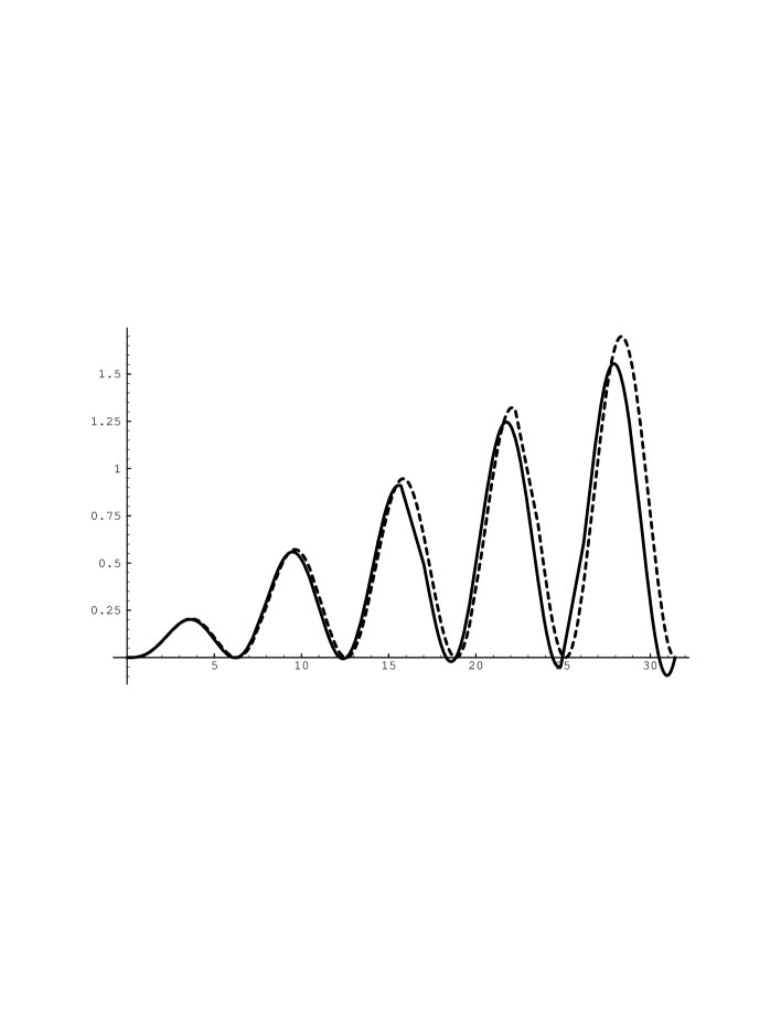
Figure 2: Graph of $f(\Delta_{31},\epsilon)$ for $\epsilon=0.03$. The solid line and the dashed line represent the exact expression eq.(35) and the approximated one eq.(59), respectively. The approximated $f$ has peaks at $\Delta_{31}=3.67,9.63,15.8,\cdots$ irrespectively of $\epsilon$.

$\Delta_{31}$	$f/\epsilon$	$\left<f/\epsilon\right>_{10\%}$	$\left<f/\epsilon\right>_{20\%}$
3.67	6.84	6.75	6.48
9.63	19.1	17.6	14.0
15.8	31.5	25.7	15.6
⋮	⋮	⋮	⋮

Table 1: The peak values of $f(\Delta_{31},\epsilon)/\epsilon$ and the corresponding averaged values. Here $\left<f/\epsilon\right>_{20\%(10\%)}$ is a value of $f(\Delta_{31},\epsilon)/\epsilon$ averaged over the range $0.8\Delta_{31}\sim 1.2\Delta_{31}$ ($0.9\Delta_{31}\sim 1.1\Delta_{31}$).

We show in Fig.2 the graph of $f(\Delta_{31},\delta m_{21}/\delta m_{31}=0.03)$. The approximation eq.(59) works very well up to $|\epsilon\Delta_{31}|\sim 1$. In the following we will use eq.(59) instead of eq.(35). We see many peaks of $f(\Delta_{31},\epsilon)$ in Fig.2. In practice, however, we do not see such sharp peaks but observe the value averaged around there, for $\Delta_{31}$ has a spread due to the energy spread of neutrino beam ($|\delta\Delta_{31}/\Delta_{31}|=|\delta E/E|$). In the following we will assume $|\delta\Delta_{31}/\Delta_{31}|=|\delta E/E|=20\%$ [33] as a typical value.

Table 1 gives values of $f(\Delta_{31},\epsilon)/\epsilon$ at the first several peaks and the averaged values around there.

We see the $T$-violation effect,

$$\left<P(\nu_{\alpha}\rightarrow\nu_{\beta})-P(\nu_{\beta}\rightarrow\nu_{\alpha})\right>_{20\%}=4J\left<f\right>_{20\%}=J\epsilon\times\left\{\begin{array}[]{c}25.9\\ 56.0\\ 62.4\\ \vdots\end{array}\right.$$ (60)

for

$$\Delta_{31}=\left\{\begin{array}[]{c}3.67\\ 9.63\\ 15.8\\ \vdots\end{array}\right.$$ (61)

at peaks for neutrino beams with 20% of energy spread. Note that the averaged peak values decrease with the spread of neutrino energy.

It depends on $\delta m_{31}^{2},L$ and $E$ which peak we can reach. The first peak $\Delta_{31}=3.67$ is reached, for example, by $\delta m_{31}^{2}=10^{-2}$ eV², $L=250$ km (for KEK/Super-Kamiokande long baseline experiments) and neutrino energy $E=1.73$ GeV. In this case we see the $T$-violation effect at best of $|25.9J\epsilon|\leq 2.50\epsilon$ since we have a bound on $J$ as eq.(38).

4.3 “$CP$ Violation”

In practice only $\nu_{\mu}$ and $\bar{\nu}_{\mu}$ are available by accelerator. It is therefore of practical importance to consider pure $CP$-violation effect through the observation of “$CP$ violation”, i.e. difference between $P(\nu_{\alpha}\rightarrow\nu_{\beta})$ and $P(\bar{\nu}_{\alpha}\rightarrow\bar{\nu}_{\beta})$.

Recalling that $P(\bar{\nu}_{\alpha}\rightarrow\bar{\nu}_{\beta})$ is obtained from $P(\nu_{\alpha}\rightarrow\nu_{\beta})$ by the replacements $a\rightarrow-a$ and $\delta\rightarrow-\delta$, we have

$$\Delta P(\nu_{\mu}\rightarrow\nu_{\rm e}) \equiv P(\nu_{\mu}\rightarrow\nu_{\rm e};L)-P(\bar{\nu}_{\mu}\rightarrow\bar{\nu}_{\rm e};L)$$ (62)

$$= \Delta P_{1}(\nu_{\mu}\rightarrow\nu_{\rm e})+\Delta P_{2}(\nu_{\mu}\rightarrow\nu_{\rm e})+\Delta P_{3}(\nu_{\mu}\rightarrow\nu_{\rm e})$$

with

$$\Delta P_{1}(\nu_{\mu}\rightarrow\nu_{\rm e}) = 16\frac{a}{\delta m^{2}_{31}}\sin^{2}\frac{\delta m^{2}_{31}L}{4E}c_{\phi}^{2}s_{\phi}^{2}s_{\psi}^{2}(1-2s_{\phi}^{2}),$$ (63)

$$\Delta P_{2}(\nu_{\mu}\rightarrow\nu_{\rm e}) = -4\frac{aL}{2E}\sin\frac{\delta m^{2}_{31}L}{2E}c_{\phi}^{2}s_{\phi}^{2}s_{\psi}^{2}(1-2s_{\phi}^{2}),$$ (64)

and

$$\Delta P_{3}(\nu_{\mu}\rightarrow\nu_{\rm e}) = -8\frac{\delta m^{2}_{21}L}{2E}\sin^{2}\frac{\delta m^{2}_{31}L}{4E}s_{\delta}c_{\phi}^{2}s_{\phi}c_{\psi}s_{\psi}c_{\omega}s_{\omega}.$$ (65)

Similarly we obtain

$$\Delta P(\nu_{\mu}\rightarrow\nu_{\mu})$$ (66)

$$= 16\frac{a}{\delta m^{2}_{31}}\left[\sin^{2}\frac{\delta m^{2}_{31}L}{4E}-\frac{1}{4}\frac{\delta m^{2}_{31}L}{2E}\sin\frac{\delta m^{2}_{31}L}{2E}\right]c_{\phi}^{2}s_{\phi}^{2}s_{\psi}^{2}\left(1-2c_{\phi}^{2}s_{\psi}^{2}\right)$$

and

$$\Delta P(\nu_{\mu}\rightarrow\nu_{\tau})$$ (67)

$$= -32\frac{a}{\delta m^{2}_{31}}\left[\sin^{2}\frac{\delta m^{2}_{31}L}{4E}-\frac{1}{4}\frac{\delta m^{2}_{31}L}{2E}\sin\frac{\delta m^{2}_{31}L}{2E}\right]c_{\phi}^{4}s_{\phi}^{2}c_{\psi}^{2}s_{\psi}^{2}$$

$$+ 8\frac{\delta m^{2}_{21}L}{2E}\sin^{2}\frac{\delta m^{2}_{31}L}{4E}s_{\delta}c_{\phi}^{2}s_{\phi}c_{\psi}s_{\psi}c_{\omega}s_{\omega}.$$

Here we make some comments.

1. $P(\nu_{\alpha}\rightarrow\nu_{\beta})$’s and $\Delta P(\nu_{\alpha}\rightarrow\nu_{\beta})$’s depend on $L$ and $E$ as functions of $L/E$ apart from the matter effect factor $a\,(=2\sqrt{2}G_{\rm F}n_{\rm e}E)$.

2. At least four experimental data are necessary to determine the function $\Delta P(\nu_{\mu}\rightarrow\nu_{\rm e})$, since it has four unknown factors: $\delta m^{2}_{31},\delta m^{2}_{21},c_{\phi}^{2}s_{\phi}^{2}s_{\psi}^{2}(1-2s_{\phi}^{2})$ and $s_{\delta}c_{\phi}^{2}s_{\phi}c_{\psi}s_{\psi}c_{\omega}s_{\omega}$. In order to determine all the mixing angles and the $CP$ violating phase, we need to observe $P(\nu_{\mu}\rightarrow\nu_{\mu})$ and $P(\bar{\nu}_{\mu}\rightarrow\bar{\nu}_{\mu})$ in addition.

3. $\Delta P(\nu_{\mu}\rightarrow\nu_{\mu})$ is independent of $\delta$ and consists only of matter effect term.

“$CP$ violation”, the difference between $P(\nu_{\alpha}\rightarrow\nu_{\beta})$ and $P(\bar{\nu}_{\alpha}\rightarrow\bar{\nu}_{\beta})$, consists of two effects: pure $CP$-violation effect and matter effect. We now investigate how we can divide $\Delta P(\nu_{\mu}\rightarrow\nu_{\rm e})$ into a pure $CP$-violation part and a matter effect part. The terms $\Delta P_{1}(\nu_{\mu}\rightarrow\nu_{\rm e})$ and $\Delta P_{2}(\nu_{\mu}\rightarrow\nu_{\rm e})$, which are proportional to “$a$”, are due to effect of the matter along the path. The term $\Delta P_{3}(\nu_{\mu}\rightarrow\nu_{\rm e})$, which is proportional to $s_{\delta}$, represents the pure $CP$ violation and indeed coincides with the $T$ violation, eq.(57) (We simply call $\Delta P_{i}(\nu_{\mu}\rightarrow\nu_{\rm e})$ as $\Delta P_{i}$ hereafter). In the following we introduce two methods to separate the pure $CP$ violating effect $\Delta P_{3}$ from the matter effect $\Delta P_{1}+\Delta P_{2}$.

4.3.1 Observation of Envelope Patterns

One method is to observe the pattern of the envelope of $\Delta P$, and to separate $\Delta P_{3}$ from it. Considering the energy dependence of $a(\propto E)$, we see that $\Delta P_{1}/L$, $\Delta P_{2}/L$ and $\Delta P_{3}$ depend on a variable $L/E$ alone. The dependences of them on the variable $L/E$, however, are different from each other as seen in Fig. 3. Each of them oscillates with common zeros at $L/E=2\pi n/\delta m^{2}_{31}(n=0,1,2,\cdots)$ and has its characteristic envelope. The envelope of $\Delta P_{1}/L$ decreases monotonously. That of $\Delta P_{2}/L$ is flat. That of $\Delta P_{3}$ increases linearly.

\begin{picture}(15.0,5.0)\centerline{\hbox{ \epsfbox{x-1sinx.eps} }} \end{picture}

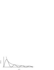
(a) Matter effect term $\Delta P_{1}(\nu_{\mu}\rightarrow\nu_{\rm e})$ divided by $L$ for $c_{\phi}^{2}s_{\phi}^{2}s_{\psi}^{2}(1-2s_{\phi}^{2})>0$. The envelope decreases monotonously with $L/E$.

\begin{picture}(15.0,5.0)\centerline{\hbox{ \epsfbox{sinx.eps} }} \end{picture}

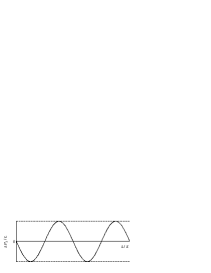
(b) Matter effect term $\Delta P_{2}(\nu_{\mu}\rightarrow\nu_{\rm e})$ divided by $L$ for $c_{\phi}^{2}s_{\phi}^{2}s_{\psi}^{2}(1-2s_{\phi}^{2})>0$. The envelope is flat.

\begin{picture}(15.0,5.0)\centerline{\hbox{ \epsfbox{xsinx.eps} }} \end{picture}

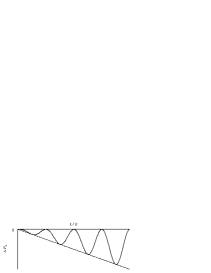
(c) $CP$-violation effect term $\Delta P_{3}(\nu_{\mu}\rightarrow\nu_{\rm e})$ for $s_{\delta}c_{\phi}^{2}s_{\phi}c_{\psi}s_{\psi}c_{\omega}s_{\omega}>0$. The envelope increases linearly with $L/E$.

Figure 3: The oscillation behaviors of the $\Delta P_{1},\Delta P_{2}$ and $\Delta P_{3}$.

It is thus possible to separate these three functions and determine $CP$ violating effect $\Delta P_{3}$ by measuring the probability $\Delta P$ over wide energy range in the long baseline neutrino oscillation experiments. This method has a merit that we can determine the pure $CP$ violating effect with a single detector.

In Fig.4 we give the probabilities $P(\nu_{\mu}\rightarrow\nu_{\rm e})$ and $P(\bar{\nu}_{\mu}\rightarrow\bar{\nu}_{\rm e})$ for a set of typical parameters which are consistent with the solar and atmospheric neutrino experiments[11]: $\delta m^{2}_{21}=10^{-4}{\rm\,eV^{2}},\delta m^{2}_{31}=10^{-2}{\rm\,eV^{2}},s_{\psi}=1/\sqrt{2},s_{\phi}=\sqrt{0.1}$ and $s_{\omega}=1/2$. We see the effect of pure $CP$ violation in Fig.4(a), since we find that the curve $\Delta P$ has the envelope characteristic of $\Delta P_{3}$.

\begin{picture}(13.0,9.0)\centerline{\hbox{ \epsfbox{mu2emax.eps} }} \end{picture}

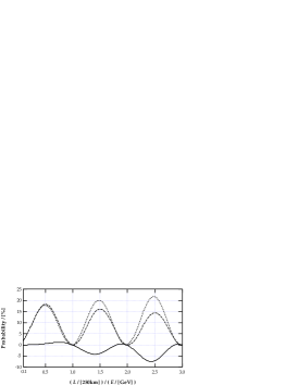
(a) The oscillation probabilities as functions of $L/E$ for $\delta=\pi/2$.

\begin{picture}(13.0,7.0)\centerline{\hbox{ \epsfbox{mu2e0.eps} }} \end{picture}

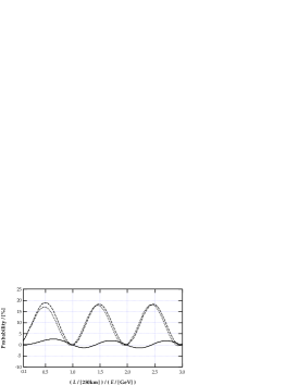
(b) The oscillation probabilities as functions of $L/E$ for $\delta=0$.

Figure 4: The oscillation probabilities for $\delta=\pi/2$ (Fig.4(a)) and $\delta=0$ (Fig.4(b)). $P(\nu_{\mu}\rightarrow\nu_{\rm e}),P(\bar{\nu}_{\mu}\rightarrow\bar{\nu}_{\rm e})$ and $\Delta P(\nu_{\mu}\rightarrow\nu_{\rm e})$ are given by a broken line, a dotted line and a solid line, respectively. Here $\rho=2.34{\rm\,g/cm^{3}}$ and $L=250{\rm\,km}$ (the distance between KEK and Super-Kamiokande) are taken. Other parameters are fixed at the following values which are consistent with the solar and atmospheric neutrino experiments [11]: $\delta m^{2}_{21}=10^{-4}{\rm\,eV^{2}},\delta m^{2}_{31}=10^{-2}{\rm\,eV^{2}},s_{\psi}=1/\sqrt{2},s_{\phi}=\sqrt{0.1}$ and $s_{\omega}=1/2$.

We comment that the envelope behavior of $\Delta P$ can be understood rather simply: Since $\Delta P_{3}$ represents the pure $CP$ violation, which is same as the $T$-violation effect in the lowest order of the matter effect,

$$\Delta P_{3}\propto f\simeq 2\Delta_{21}\sin^{2}\frac{\Delta_{31}}{2}.$$ (68)

(See the discussion above the eq.(59)). This shows $\Delta P_{3}$ has a linearly increasing envelope $\Delta_{21}\propto L/E$. On the other hand, the envelopes of $\Delta P_{1}$ and $\Delta P_{2}$ do not increase with $L/E$ for fixed $L$, and it makes $\Delta P_{3}$ dominant in $\Delta P$ for large $L/E$.

Such characters of envelope behaviors enables us to determine whether $CP$-violation effect is present or not even in case neutrino beam has energy spread; for neutrino with widely spread energy spectrum, we observe the average of “$CP$-violation” effect which is not zero if there is pure $CP$-violation effect (see Fig.4).

4.3.2 Comparison of Experiments with Different $L$’s

The other method is to separate the pure $CP$ violating effect by comparison of experiments with two different $L$’s. Suppose that two experiments, one with $L=L_{1}$ and the other $L=L_{2}$, are available. We observe two probabilities $P(\nu_{\mu}\rightarrow\nu_{\rm e};E_{1},L_{1})$ and $P(\nu_{\mu}\rightarrow\nu_{\rm e};E_{2},L_{2})$ with $L_{1}/E_{1}=L_{2}/E_{2}$. Recalling that $P(\nu_{\mu}\rightarrow\nu_{\rm e};L)$ is a function of $L/E$ apart from the matter effect factor $a(\propto E)$, we see that the difference

$$\left\{P(\nu_{\mu}\rightarrow\nu_{\rm e};E_{1},L_{1})-P(\nu_{\mu}\rightarrow\nu_{\rm e};E_{2},L_{2})\right\}_{L_{1}/E_{1}=L_{2}/E_{2}}$$ (69)

is due only to terms proportional to “$a$”. We obtain $\Delta P_{3}$ by subtracting these terms ($\Delta P_{1}+\Delta P_{2}$) from $\Delta P(\nu_{\mu}\rightarrow\nu_{\rm e})$ as

$$\Delta P_{3}(\nu_{\mu}\rightarrow\nu_{\rm e};E_{1},L_{1})$$ (70)

$$= \left[\Delta P(\nu_{\mu}\rightarrow\nu_{\rm e};E_{1},L_{1})-\frac{2L_{1}}{L_{2}-L_{1}}\left\{P(\nu_{\mu}\rightarrow\nu_{\rm e};E_{2},L_{2})-P(\nu_{\mu}\rightarrow\nu_{\rm e};E_{1},L_{1})\right\}\right]_{L/E={\rm const.}}$$

$$= \left[\Delta P(\nu_{\mu}\rightarrow\nu_{\rm e};E_{1},L_{1})-\frac{L_{1}}{L_{2}-L_{1}}\left\{\Delta P(\nu_{\mu}\rightarrow\nu_{\rm e};E_{2},L_{2})-\Delta P(\nu_{\mu}\rightarrow\nu_{\rm e};E_{1},L_{1})\right\}\right]_{L/E={\rm const.}}.$$ (71)

This method has a merit that it does not need to observe the envelope nor many oscillation bumps in the low energy range.

In Fig.5 we compare $P(\nu_{\mu}\rightarrow\nu_{\rm e})$ for $L=250{\rm km}$ (KEK/Super-Kamiokande experiment) with that for $L=730{\rm km}$ (Minos experiment) in a case with the same neutrino masses and mixing angles as those in Fig.4(a). We see their difference, consisting only of the matter effect, has the same shape as the solid line in Fig. 4(b) up to a overall constant. We also show the pure $CP$ violating effect obtained by the two probabilities with eq.(70). This curve has a linearly increasing envelope as seen in Fig. 3(c).

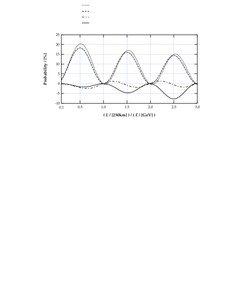
Figure 5: The oscillation probabilities $P(\nu_{\mu}\rightarrow\nu_{\rm e})$’s for KEK/Super-Kamiokande experiments with $L=250{\rm km}$ (broken line) and those for Minos experiments with $L=730{\rm km}$ (dotted line). Masses and mixing angles are the same as in Fig. 4(a). Their difference, which consists only of matter effect, is shown by a dot-dashed line. The pure $CP$ violating effect in KEK/Super-Kamiokande experiments determined by eq.(70) is drawn by a solid line.

In this section we have shown that it is possible to determine the $CP$-violation effect in case $\delta m^{2}$’s have small values of ${\cal O}(10^{-4}{\rm eV^{2}})$ and ${\cal O}(10^{-2}\;{\rm eV}^{2})$, respecting solar neutrino deficit and atmospheric neutrino anomaly. Even in this case we may see about 5% or more $CP$-violation effect in the near future.

5 Summary and Discussions

We have examined the $CP$ and $T$ violation in the neutrino oscillation and analyzed how large the violation can be, taking into account the solar neutrino deficit and the atmospheric neutrino anomaly.

In case of the comparable mass differences with $\delta m^{2}_{21},\delta m^{2}_{31}$ and $\delta m^{2}_{32}$ in the range $10^{-3}$ to $10^{-2}{\rm eV^{2}}$, which is consistent with the analysis of the atmospheric neutrino anomalies (and maybe with the solar neutrino deficit), it is found that there is a possibility that the $CP$ violation effect is large enough to be observed by 100 $\sim$ 1000 km baseline experiments if the $CP$ violating parameter sin$\delta$ is sufficiently large.

In case that $\delta m^{2}_{21}$ is much smaller than $\delta m^{2}_{31}$, which is favored if we attribute both the solar and atmospheric neutrino anomalies to the neutrino oscillation, the matter effect by the earth gives the effective mass equal or greater than the smaller mass difference $\delta m^{2}_{21}$ and we cannot ignore the presence of matter.

We have given very simple formulae for the transition probabilities of neutrinos in long baseline experiments for this case. They have taken into account not only the $CP$-violation effect but also the matter effect, and are applicable to such interesting parameter regions that can explain both the atmospheric neutrino anomaly and the solar neutrino deficit by the neutrino oscillation.

With these simple expressions we have shown that measurement of the $T$ violation gives the pure $CP$ violating effect.

We have also shown with the aid of these formulae two methods to distinguish pure $CP$ violation from matter effect. The dependence of pure $CP$-violation effect on the energy $E$ and the distance $L$ is different from that of matter effect: The former depends on $L/E$ alone and has a form $f(L/E)$, while the latter has a form $L\times g_{1}(L/E)\equiv E\times g_{2}(L/E)$. One method to distinguish is to observe closely the energy dependence of the difference $P(\nu_{\mu}\rightarrow\nu_{\rm e};L)-P(\bar{\nu}_{\mu}\rightarrow\bar{\nu}_{\rm e};L)$ including the envelope of oscillation bumps. The other is to compare results from two different distances $L_{1}$ and $L_{2}$ with $L_{1}/E_{1}=L_{2}/E_{2}$ and then to subtract the matter effect by eq.(70) or eq.(71).

Each method has both its merits and demerits. The first one has a merit that we need experiments with only a single detector. A merit of the second is that we do not need wide range of energy (many bumps) to survey the neutrino oscillation.

It is desirable to make long baseline neutrino oscillation experiments with high intensity neutrino flux, and to study $CP$ violation in the lepton sector experimentally. Even if the mass differences are very disparate we may see about 5% or more $CP$ violation as is seen from Fig.4 and Fig.5.

Appendix Appendix A Derivation of the Oscillation Probabilities

Here we present the derivation of eq.(54) $\sim$ eq.(56) with use of eq.(53), and show how well this approximation works. Let us set $S(x)=S_{0}(x)+S_{1}(x)$, defining

$$S_{0}(x) = {\rm e}^{-{\rm i}H_{0}x},$$ (A1)

$$S_{1}(x) = {\rm e}^{-{\rm i}H_{0}x}({\rm-i})\int_{0}^{x}{\rm d}sH_{1}(s).$$ (A2)

We see

$$S_{0}(x)_{\beta\alpha} = \left\{U{\rm e}^{-{\rm i}\frac{x}{2E}{\rm diag}(0,0,\delta m^{2}_{31})}U^{\dagger}\right\}_{\beta\alpha}$$ (A3)

$$= \delta_{\beta\alpha}+U_{\beta 3}U^{\ast}_{\alpha 3}({\rm e}^{-{\rm i}\frac{\delta m^{2}_{31}x}{2E}}-1)$$

and

$$S_{1}(x)_{\beta\alpha} = -{\rm i}\int_{0}^{x}{\rm d}s\,\left[{\rm e}^{-{\rm i}H_{0}(x-s)}H_{1}{\rm e}^{-{\rm i}H_{0}s}\right]_{\beta\alpha}$$ (A4)

$$= -{\rm i\,}U_{\beta i}U^{\ast}_{\gamma i}(H_{1})_{\gamma\delta}U_{\delta j}U^{\ast}_{\alpha j}\Gamma(x)_{ij},$$

where

$$\Gamma(x)_{ij} \equiv \int_{0}^{x}{\rm d}s\,{\rm e}^{-{\rm i\,}\frac{\delta m^{2}_{31}}{2E}\{(x-s)\delta_{i3}+s\delta_{j3}\}}$$ (A5)

$$= \delta_{i3}\delta_{j3}\cdot x{\rm e}^{-{\rm i}\frac{\delta m^{2}_{31}x}{2E}}$$

$$+ \left\{(1-\delta_{i3})\delta_{j3}+\delta_{i3}(1-\delta_{j3})\right\}\cdot\left(-{\rm i}\frac{\delta m^{2}_{31}}{2E}\right)^{-1}\left({\rm e}^{-{\rm i}\frac{\delta m^{2}_{31}x}{2E}}-1\right)$$

$$+ (1-\delta_{i3})(1-\delta_{j3})\cdot x.$$

Using

$$U^{\ast}_{\gamma i}(H_{1})_{\gamma\delta}U_{\delta j} = \frac{1}{2E}\left\{{\rm diag}(0,\delta m^{2}_{21},0)+U^{\dagger}{\rm diag}(a,0,0)U\right\}_{ij}$$ (A6)

$$= \frac{\delta m^{2}_{21}}{2E}\delta_{i2}\delta_{j2}+\frac{a}{2E}U^{\ast}_{1i}U_{1j}$$

and

$$\sum_{k=1}^{2}U^{\ast}_{\alpha k}U_{1k}=\delta_{\alpha 1}-U^{\ast}_{\alpha 3}U_{13},$$ (A7)

we obtain

$$S(x)_{\beta\alpha}=\delta_{\beta\alpha}+{\rm i\,}T(x)_{\beta\alpha}$$ (A8)

with

$${\rm i\,}T(x)_{\beta\alpha} = -2{\,\rm i\,}{\rm e}^{-{\rm i}\frac{\delta m^{2}_{31}x}{4E}}\sin\frac{\delta m^{2}_{31}}{4E}U_{\beta 3}U^{\ast}_{\alpha 3}\left[1-\frac{a}{\delta m^{2}_{31}}\left(2\left|U_{13}\right|^{2}-\delta_{\alpha 1}-\delta_{\beta 1}\right)-{\rm i\,}\frac{ax}{2E}\left|U_{13}\right|^{2}\right]$$ (A9)

$$- {\rm i\,}\frac{\delta m^{2}_{31}x}{2E}\left[\frac{\delta m^{2}_{21}}{\delta m^{2}_{31}}U_{\beta 2}U^{\ast}_{\alpha 2}+\right.$$

$$\left.\frac{a}{\delta m^{2}_{31}}\left\{\delta_{\alpha 1}\delta_{\beta 1}\left|U_{13}\right|^{2}+U_{\beta 3}U^{\ast}_{\alpha 3}\left(2\left|U_{13}\right|^{2}-\delta_{\alpha 3}-\delta_{\beta 3}\right)\right\}\right].$$

We then obtain the oscillation probability in the lowest order approximation as

$$P(\nu_{\alpha}\rightarrow\nu_{\beta};L)=\left|S(L)_{\beta\alpha}\right|^{2}$$ (A10)

$$= \delta_{\beta\alpha}\left[1-4\left|U_{\alpha 3}\right|^{2}\sin^{2}\frac{\delta m^{2}_{31}L}{4E}\left\{1-2\frac{a}{\delta m^{2}_{31}}\left(\left|U_{13}\right|^{2}-\delta_{\alpha 1}\right)\right\}\right.$$

$$\left.-2\frac{aL}{2E}\sin\frac{\delta m^{2}_{31}L}{2E}\left|U_{\alpha 3}\right|^{2}\left|U_{13}\right|^{2}\right]$$

$$+ 4\left|U_{\beta 3}\right|^{2}\left|U_{\alpha 3}\right|^{2}\sin^{2}\frac{\delta m^{2}_{31}L}{4E}\left\{1-4\frac{a}{\delta m^{2}_{31}}\left|U_{13}\right|^{2}+2\frac{a}{\delta m^{2}_{31}}(\delta_{\alpha 1}+\delta_{\beta 1})\right\}$$

$$+ 2\frac{\delta m^{2}_{31}L}{2E}\sin\frac{\delta m^{2}_{31}L}{2E}\left[\frac{\delta m^{2}_{21}}{\delta m^{2}_{31}}{\,\rm Re\,}\left(U^{\ast}_{\beta 3}U_{\beta 2}U_{\alpha 3}U^{\ast}_{\alpha 2}\right)\right.$$

$$\left.+\frac{a}{\delta m^{2}_{31}}\left\{\delta_{\alpha 1}\delta_{\beta 1}\left|U_{13}\right|^{2}+\left|U_{\alpha 3}\right|^{2}\left|U_{\beta 3}\right|^{2}\left(2\left|U_{13}\right|^{2}-\delta_{\alpha 1}-\delta_{\beta 1}\right)\right\}\right]$$

$$- 4\frac{\delta m^{2}_{21}L}{2E}\sin^{2}\frac{\delta m^{2}_{31}L}{4E}{\,\rm Im\,}\left(U^{\ast}_{\beta 3}U_{\beta 2}U_{\alpha 3}U^{\ast}_{\alpha 2}\right).$$

Substituting eq.(18) in eq.(A10) we finally obtain eq.(54) $\sim$ eq.(56). Note that all the terms except the last one in eq.(A10) is invariant under the exchange of $\alpha$ and $\beta$; the last term changes its sign by this exchange. It is thus obvious that the last term gives $T$-violation effect.

\begin{picture}(15.0,8.0)\centerline{\hbox{ \epsfbox{KEKKamCompare.eps} }} \end{picture}

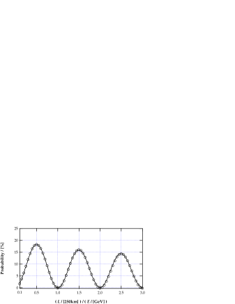
(a) Exact and approximated values of $P(\nu_{\mu}\rightarrow\nu_{\rm e})$ for $L=250$ km assuming constant matter density.

\begin{picture}(15.0,8.0)\centerline{\hbox{ \epsfbox{MinosCompare.eps} }} \end{picture}

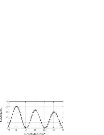
(b) Exact and approximated values of $P(\nu_{\mu}\rightarrow\nu_{\rm e})$ for $L=730$ km assuming constant matter density.

Figure 6: Exact and approximated values of $P(\nu_{\mu}\rightarrow\nu_{\rm e})$ for $L=250$ km (Fig.6(a)) and those for $L=730$ km (Fig.6(b)) assuming constant matter density. Exact values and approximated ones are shown by a solid line and white circles, respectively. The parameters $s_{\psi},s_{\phi},s_{\omega},\delta$ and $\rho$ are taken the same as in Fig. 4(a).

\begin{picture}(15.0,8.0)\centerline{\hbox{ \epsfbox{density.eps} }} \end{picture}

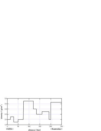
(a) Matter density profile between KEK and Super-Kamiokande[35]. Average value of the density is 2.34 g/cm³.

\begin{picture}(15.0,8.0)\centerline{\hbox{ \epsfbox{vardensity.eps} }} \end{picture}

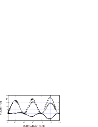
(b) Comparison of values of oscillation probabilities, considering and averaging local matter density. A broken line, a dotted line and a solid line are values of $P(\nu_{\mu}\rightarrow\nu_{\rm e})$, $P(\bar{\nu}_{\mu}\rightarrow\bar{\nu}_{\rm e})$ and $\Delta P(\nu_{\mu}\rightarrow\nu_{\rm e})$, respectively, taking the density profile shown in (a) into account. Circles, squares and triangles denote the corresponding values with constant density approximation (eq.(54)) with averaged matter density, $\rho=2.34\;{\rm g/cm^{3}}$.

Figure 7: Effect of matter density variation on $P(\nu_{\mu}\rightarrow\nu_{\rm e})$, $P(\bar{\nu}_{\mu}\rightarrow\bar{\nu}_{\rm e})$ and $\Delta P(\nu_{\mu}\rightarrow\nu_{\rm e})$. The parameters $s_{\omega},s_{\psi},s_{\phi}$ and $\delta$ are taken the same as in Fig.4(a).

Figure 6 shows how well this approximation works for KEK/Super-Kamiokande experiments and also for Minos experiments with the same masses, mixing angles and $CP$ violating phase as in Fig.4(a). Our approximation requires (see eq.(52))

$$\frac{aL}{2E}=0.420\left(\frac{L}{\rm 730\,km}\right)\left(\frac{\rho}{\rm 3\,g\,cm^{-3}}\right)\ll 1$$ (A11)

and

$$\frac{\delta m^{2}_{21}L}{2E}=0.185\frac{(\delta m^{2}_{21}/{\rm 10^{-4}eV^{2}})(L/{\rm 730km})}{E/{\rm GeV}}\ll 1,$$ (A12)

which is marginally satisfied for $L=730{\rm km}$. We see that even in this case eq.(A10) gives good approximation.

We stated that we can use an averaged value $\left<a\right>$ in place of $a$ in case matter density spatially varies. We present in Fig.7 the goodness of constant matter density approximation for KEK/Super-Kamiokande experiments.

References

- [1] GALLEX Collaboration, P. Anselmann et al., Phys. Lett. B 357, 237 (1995).
- [2] SAGE Collaboration, J. N. Abdurashitov et al., Phys. Lett. B 328, 234 (1994).
- [3] Kamiokande Collaboration, Y. Suzuki, Nucl. Phys. B (Proc. Suppl.) 38,54 (1995).
- [4] Homestake Collaboration, B. T. Cleveland et al., Nucl. Phys. B (Proc. Suppl.) 38, 47 (1995).
- [5] Kamiokande Collaboration, K.S. Hirata et al., Phys. Lett. B 205, 416 (1988); ibid. B 280, 146 (1992) ; Y. Fukuda et al., Phys. Lett. B 335, 237 (1994).
-
[6]
IMB Collaboration,
D. Casper et al., Phys. Rev. Lett. 66, 2561 (1991);
R. Becker-Szendy et al., Phys. Rev. D 46, 3720 (1992). - [7] SOUDAN2 Collaboration, T. Kafka, Nucl. Phys. B (Proc. Suppl.) 35, 427 (1994); M. C. Goodman, ibid. 38 (1995) 337; W. W. M. Allison et al., hep-ex/9611007.
- [8] NUSEX Collaboration, M. Aglietta et al., Europhys. Lett. 8, 611(1989); ibid. 15, 559 (1991).
- [9] Fréjus Collaboration, K. Daum et al., Z. Phys. C 66, 417 (1995).
- [10] G. L. Fogli, E. Lisi, D. Montanino and G. Scioscia, Phys. Rev. D 55, 4385 (1997).
- [11] G. L. Fogli, E. Lisi and D. Montanino, Phys. Rev. D 54, 2048 (1996); G. L. Fogli, E. Lisi and D. Montanino, Phys. Rev. D 49, 3626 (1994).
- [12] O. Yasuda, preprint TMUP-HEL-9603, hep-ph/9602342.
- [13] K. Nishikawa, INS-Rep-924 (1992).
- [14] S. Parke, Fermilab-Conf-93/056-T (1993), hep-ph/9304271.
- [15] M. Tanimoto, Phys. Rev. D 55, 322 (1997); M. Tanimoto, hep-ph/9612444.
- [16] J. Arafune and J. Sato, Phys. Rev. D 55, 1653 (1997).
- [17] J. Sato, hep-ph/9701306.
- [18] J. Arafune, M. Koike and J. Sato, to be published in Phys. Rev. D, hep-ph/9703351.
- [19] H. Minakata and H. Nunokawa, Preprint UWThPh-1997-11, DFTT 26/97, hep-ph/9705300; H. Minakata and H. Nunokawa, Preprint TMUP-HEL-9705, FTUV/97-31,IFIC/97-30, hep-ph/9706281.
- [20] S. M. Bilenky, C. Giunti and W. Grimus, Preprint UWThPh-1997-11, DFTT 26/97, hep-ph/9705300.
- [21] A. Acker and S. Pakvasa, Phys. Lett. B 397 209 (1997).
- [22] P. I. Krastev, Nuovo Cim. A 103, 103, 361 (1990).
- [23] For a review, M. Fukugita and T. Yanagida, in Physics and Astrophysics of Neutrinos, edited by M. Fukugita and A. Suzuki (Springer-Verlag, Tokyo, 1994).
- [24] S. M. Bilenky and S. T. Petcov, Rev. Mod. Phys. 59, 671 (1987).
- [25] S. Pakvasa, in High Energy Physics – 1980, Proceedings of the 20th International Conference on High Energy Physics, Madison, Wisconsin, edited by L. Durand and L. Pondrom, AIP Conf. Proc. No. 68 (AIP, New York, 1981), Vol. 2, pp. 1164.
- [26] L. -L. Chau and W. -Y. Keung, Phys. Rev. Lett. 59, 671 (1987).
- [27] T. K. Kuo and J. Pantaleone, Phys. Lett. B 198, 406 (1987).
- [28] S. Toshev, Phys. Lett. B 226, 335 (1989).
- [29] L. Wolfenstein, Phys. Rev. D 17, 2369 (1978).
- [30] S. P. Mikheev and A. Yu. Smirnov, Sov. J. Nucl. Phys. 42, 913 (1985).
- [31] V. Barger, K. Whisnant and R. J. N. Phillips, Phys. Rev. Lett. 45, 2084 (1980).
- [32] N. Cabibbo, Phys. Lett. B 72, 333 (1978).
- [33] K. Nishikawa, Private communication.
- [34] LSND Collaboration, C. Athanassopoulos et al., Phys. Rev. C 54, 2685 (1996); Phys. Rev. Lett. 77, 3082 (1996); ibid. 75, 2650 (1995).
- [35] M. Komazawa, Private communication.