Low-Energy Constraints on New Physics Revisited

Abstract

It is possible to place constraints on non-Standard-Model gauge-boson self-couplings and other new physics by studying their one-loop contributions to precisely measured observables. We extend previous analyses which constrain such nonstandard couplings, and we present the results in a compact and transparent form. Particular attention is given to comparing results for the light-Higgs scenario, where nonstandard effects are parameterized by an effective Lagrangian with a linear realization of the electroweak symmetry breaking sector, and the heavy-Higgs/strongly interacting scenario, described by the electroweak chiral Lagrangian. The constraints on nonstandard gauge-boson self-couplings which are obtained from a global analysis of low-energy data and LEP/SLC measurements on the $Z$ pole are updated and improved from previous studies.

I Introduction

Due to the extraordinary precision of electroweak data at low energy and on the $Z$ pole it is possible to place constraints on models for physics beyond the Standard Model (SM) by studying the loop-level contributions of the new physics to electroweak observables. Gauge-boson self-interactions are a fascinating aspect of the SM, and the exploration of this sector is still in its early stages. While this sector is important in its own right, it is intimately related to the symmetry-breaking sector of the SM. Hence, we are strongly motivated to garner from the body of electroweak precision data any and all available clues concerning these heretofore more poorly understood sectors of the SM.

Currently all available precision data concerns processes with four external light fermions (such as $e^{+}e^{-}\rightarrow Z^{*}\rightarrow f\overline{f}$ at LEP). We follow the scheme of Ref. [1] which organizes the calculation of these amplitudes in the following manner. First we calculate $\Pi_{T}^{\gamma\gamma}(q^{2})$, $\Pi_{T}^{\gamma Z}(q^{2})$, $\Pi_{T}^{ZZ}(q^{2})$ and $\Pi_{T}^{WW}(q^{2})$, i.e. the transverse components of the $\gamma\gamma$, $\gamma Z$, $ZZ$ and $WW$ two-point-functions, respectively. As well we must calculate $\Gamma^{ff\gamma}(q^{2})$, $\Gamma^{ffZ}(q^{2})$ and $\Gamma^{ff^{\prime}W}(q^{2})$, i.e. corrections to the gauge-boson-fermion vertices. The two-point-functions and a portion of the vertex corrections are combined via the pinch technique[2, 3, 4, 5] to form the gauge-invariant effective charges, $\overline{e}^{2}(q^{2})$, $\overline{s}^{2}(q^{2})$, $\overline{g}_{Z}^{2}(q^{2})$ and $\overline{g}_{W}^{2}(q^{2})$. These effective charges contain the major part of the higher order corrections and are universal to all four-fermion amplitudes. (Hence, this approach is especially well suited to a global analysis of electroweak precision data.) The calculation of the four-fermion amplitudes is then completed by adding the process-dependent vertex and box corrections. A more complete discussion is given in Section II. In fact, most of the technical details are provided in Section II, which allows us to be very much to the point in the ensuing sections.

In the context of this paper all of the non-SM contributions enter via the effective charges plus a form factor for the $Zb\overline{b}$ vertex. With the exception of this latter form factor, the vertex and box corrections reduce to their SM values for the quantities we compute. This greatly simplifies the analysis.

In Section III the SM Lagrangian is extended by the addition of energy-dimension-six (${\cal O}(E^{6})\,$) operators. The operators are constructed from the fields of the low-energy spectrum including the usual SU(2) Higgs doublet of the SM, i.e. spontaneous symmetry breaking (SSB) is linearly realized. The effective charges and the $Zbb$-vertex form factor, $\overline{\delta}_{b}$[1], are calculated in this scheme. In Section IV the electroweak chiral Lagrangian, in which there is no physical Higgs boson and the symmetry breaking is nonlinearly realized[6], is discussed, and we repeat the calculation of the effective charges and $\overline{\delta}_{b}$. Then, in Section V, we specialize to a discussion of non-Abelian gauge boson couplings.

Numerical results are given in Section VI. We pay particular attention to the uncertainties inherent in obtaining bounds on new physics from one-loop effects. First, the sensitivity of the data to the parameters of the effective Lagrangians of Section III and Section IV is estimated by considering the contributions of only one new operator at a time. Then, bounds on non-SM contributions to gauge-boson self-couplings are presented accounting for limited correlations. Additionally we consider some more complicated scenarios, and we compare the results from both the linear and the nonlinear models.

II Low-energy parameters and effective charges

We begin by calculating the corrections to the gauge-boson two-point-functions as depicted by Fig. 1. Introducing the transverse and longitudinal

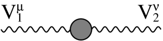
FIG. 1.: Higher-order contributions to the $V_{1}^{\mu}V_{2}^{\nu}$ two-point-functions; $V_{1}V_{2}$ denotes $\gamma\gamma$, $\gamma Z$, $ZZ$ or $WW$. Generically the ‘blob’ may represent a contact term, a ‘bubble’ or a ‘tadpole’.

projection operators

$$P_{T}^{\mu\nu}=g^{\mu\nu}-\frac{q^{\mu}q^{\nu}}{q^{2}}\;,\makebox[28.45274pt]{}P_{L}^{\mu\nu}=\frac{q^{\mu}q^{\nu}}{q^{2}}\;,$$ (1)

which possess the desirable properties

$$P_{T}^{\mu\nu}+P_{L}^{\mu\nu}=g^{\mu\nu},\makebox[14.22636pt]{}P_{T\alpha}^{\mu}P_{T}^{\alpha\nu}=P_{T}^{\mu\nu},\makebox[14.22636pt]{}P_{L\alpha}^{\mu}P_{L}^{\alpha\nu}=P_{L}^{\mu\nu},\makebox[14.22636pt]{}P_{T\alpha}^{\mu}P_{L}^{\alpha\nu}=0=P_{L\alpha}^{\mu}P_{T}^{\alpha\nu},$$ (2)

we may write the result of the calculation of Fig. 1 as

$$-i\Pi^{\mu\nu}_{V_{1}V_{2}}(q^{2})=-i\Pi^{V_{1}V_{2}}_{T}(q^{2})P_{T}^{\mu\nu}-i\Pi^{V_{1}V_{2}}_{L}(q^{2})P_{L}^{\mu\nu}\;,$$ (3)

where $q^{2}$ is the four-momentum squared of the propagating gauge bosons. Since we are considering processes where the gauge-boson propagators are coupled to massless fermion currents, we need to consider only the transverse contribution, $\Pi^{V_{1}V_{2}}_{T}(q^{2})$; the longitudinal contributions don’t contribute by the Dirac equation for massless fermions. Equivalently we can calculate $-i\Pi^{\mu\nu}_{V_{1}V_{2}}(q^{2})$ and retain only the coefficient of $-ig^{\mu\nu}$.

Next, we calculate vertex corrections as depicted in Fig. 2.

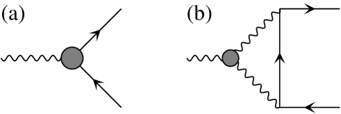
FIG. 2.: Higher-order contributions to the $Vf_{1}f_{2}$ vertex where $V=\gamma$, $Z$ or $W$. Generically the ‘blob’ in (a) denotes a large variety of graphs. However, for the new-physics contributions which we discuss, all contributions arise from graphs of type (b).

Using the pinch technique, a portion of the vertex corrections in Fig. 2(a) are combined with the two-point-function corrections. This standard technique[2, 3, 4, 5] renders propagator and vertex corrections separately gauge invariant. Furthermore, large cancellations which would occur between the propagator and vertex contributions are avoided.

For the SM contributions we use the results of Ref. [1]. For the new-physics contributions which we consider in later sections the discussion is very simple. All new-physics contributions are of the type depicted in Fig. 2(b), where the ‘blob’ denotes some nonstandard contribution to the $WW\gamma$ or $WWZ$ vertex. These corrections can be divided into two pieces. One piece, which is independent of any fermion masses, is purely pinch term; the remaining contributions, which depend on the fermion masses, will remain as part of the vertex corrections. We will discuss these latter corrections later in this section.

For the moment we neglect the contributions of fermion masses, and, following Ref. [7], we write

$$-i\Delta\Gamma_{\mu}^{\gamma f_{1}f_{2}}(q) = -i\gamma_{\mu}\frac{1}{2}(1-\gamma_{5})\hat{g}I_{3}^{f}\Delta\Gamma_{L}^{\gamma}(q^{2})\;,$$ (5)

$$-i\Delta\Gamma_{\mu}^{Zf_{1}f_{2}}(q) = -i\gamma_{\mu}\frac{1}{2}(1-\gamma_{5})\hat{g}I_{3}^{f}\Delta\Gamma_{L}^{Z}(q^{2})\;,$$ (6)

$$-i\Delta\Gamma_{\mu}^{Wf_{1}f_{2}}(q) = -i\gamma_{\mu}\frac{1}{2}(1-\gamma_{5})\frac{\hat{g}}{\sqrt{2}}\Delta\Gamma_{L}^{W}(q^{2})\;,$$ (7)

where $I_{3}^{f}=\pm\frac{1}{2}$ is the third component of weak isospin for the external fermion. The notation on the left-hand side should be clear from the superscripts. Here and through the remainder of the paper we separate various quantities according to $X=X_{\rm SM}+\Delta X$. Hence, above, $\Delta\Gamma$ is the contribution of the new physics to the vertex correction, $\Gamma$ (indices suppressed for brevity). All ‘hatted’ couplings are the $\overline{\rm MS}$ couplings, and hence they satisfy the tree-level relations $\hat{e}=\hat{g}\hat{s}=\hat{g}_{Z}\hat{s}\hat{c}$ and $\hat{e}^{2}=4\pi\hat{\alpha}$. In particular, $\hat{g}$ is the SU(2) coupling, $\hat{s}$ and $\hat{c}$ are the sine and cosine of the weak mixing angle, and the strength of the photon coupling is given by $\hat{e}$ or $\hat{\alpha}$. Finally, the U(1) coupling is given by $\hat{g}^{\prime}=\hat{g}\hat{s}/\hat{c}$.

Notice in Eqn. (2) that the corrections are purely left-handed due to the coupling of at least one $W$ boson to the fermion line, hence we have extracted a factor of $\frac{1}{2}(1-\gamma_{5})$ on the right-hand side. The appearance of the factor $I_{3}^{f}$ in Eqns. (5)-(6) may be understood as follows. For corrections to the $WW\gamma$ or $WWZ$ vertex due to the type of loop graph depicted in Figure 2(b), there are two internal $W$ bosons, one of each charge, connected to an external photon or $Z$ boson through a $WW\gamma$ or $WWZ$ vertex. If the external fermion legs are up-type quarks, then the internal fermion is a down-type quark (and vice versa). Interchanging the up-type and down-type quarks interchanges the $W^{+}$ and $W^{-}$, which, due to the properties of the $WW\gamma$ or $WWZ$ vertex, leads to an overall sign change. Of course the same argument applies if the quarks are replaced by neutrinos and charged leptons. An additional coupling factor is extracted for convenience, leaving finally the process-independent scalar form factors $\Delta\Gamma_{L}^{\gamma}(q^{2})$, $\Delta\Gamma_{L}^{Z}(q^{2})$ and $\Delta\Gamma_{L}^{W}(q^{2})$ on the right-hand side. Finally, we form the combinations

$$\Delta\overline{\Pi}_{T}^{\gamma\gamma}(q^{2}) = \Delta\Pi_{T}^{\gamma\gamma}(q^{2})-2\hat{s}q^{2}\Delta\Gamma_{L}^{\gamma}(q^{2})\;,$$ (9)

$$\Delta\overline{\Pi}_{T}^{\gamma Z}(q^{2}) = \Delta\Pi_{T}^{\gamma Z}(q^{2})-\hat{s}q^{2}\Delta\Gamma_{L}^{Z}(q^{2})-\hat{c}(q^{2}-m_{Z}^{2})\Delta\Gamma_{L}^{\gamma}(q^{2})\;,$$ (10)

$$\Delta\overline{\Pi}_{T}^{ZZ}(q^{2}) = \Delta\Pi_{T}^{ZZ}(q^{2})-2\hat{c}(q^{2}-m_{Z}^{2})\Delta\Gamma_{L}^{Z}(q^{2})\;,$$ (11)

$$\Delta\overline{\Pi}_{T}^{WW}(q^{2}) = \Delta\Pi_{T}^{WW}(q^{2})-2(q^{2}-m_{W}^{2})\Delta\Gamma_{L}^{W}(q^{2})\;,$$ (12)

where the $\overline{\Pi}_{T}^{V_{1}V_{2}}(q^{2})$’s on the left-hand side are now gauge-invariant expressions.

The contributions of these two-point-functions to four-fermion amplitudes is generally summarized by a set of parameters such as the $S$, $T$ and $U$ parameters of Ref. [8] or an equivalent set[9]. Following Ref. [1] we define

$$\alpha\Delta S = 4\hat{s}^{2}\hat{c}^{2}\bigg{\{}-\Delta\overline{\Pi}_{T,Z}^{ZZ}(0)+\frac{\hat{c}^{2}-\hat{s}^{2}}{\hat{s}\hat{c}}\Delta\overline{\Pi}_{T,\gamma}^{\gamma Z}(m_{Z}^{2})+\Delta\overline{\Pi}_{T,\gamma}^{\gamma\gamma}(m_{Z}^{2})\bigg{\}}\;,$$ (14)

$$\alpha\Delta T = \frac{\Delta\overline{\Pi}_{T}^{ZZ}(0)}{m_{Z}^{2}}-\frac{\Delta\overline{\Pi}_{T}^{WW}(0)}{m_{W}^{2}}\;,$$ (15)

$$\alpha\Delta U = 4\hat{s}^{2}\bigg{\{}\hat{c}^{2}\Delta\overline{\Pi}_{T,Z}^{ZZ}(0)-\Delta\overline{\Pi}_{T,W}^{WW}(0)+\hat{s}^{2}\Delta\overline{\Pi}_{T,\gamma}^{\gamma\gamma}(m_{Z}^{2})+2\hat{s}\hat{c}\Delta\overline{\Pi}_{T,\gamma}^{\gamma Z}(m_{Z}^{2})\bigg{\}}\;,$$ (16)

where

$$\overline{\Pi}^{V_{1}V_{2}}_{T,V_{3}}(q^{2})={\overline{\Pi}^{V_{1}V_{2}}_{T}(q^{2})-\overline{\Pi}^{V_{1}V_{2}}_{T}(m^{2}_{V_{3}})\over q^{2}-m^{2}_{V_{3}}}\;.$$ (17)

Notice the different subscripts on the left-hand and right-hand sides of Eqn. (17).

Several points concerning the usage of $\Delta S$, $\Delta T$ and $\Delta U$ should be made. First of all, we may expand the $\overline{\Pi}$ functions in a power series in $q^{2}$ according to

$$\Delta\overline{\Pi}^{V_{1}V_{2}}_{T}(q^{2})=A^{V_{1}V_{2}}+q^{2}\,B^{V_{1}V_{2}}+(q^{2})^{2}\,C^{V_{1}V_{2}}+...\;.$$ (18)

If we include only the $A$ and $B$ coefficients in our expansion, then, considering all four $\overline{\Pi}$ functions, there are a total of eight constant coefficients. By a Ward identity, $A^{\gamma\gamma}=A^{\gamma Z}=0$. Using the three physical input parameters (for which we choose $\alpha$, $m_{Z}$ and $G_{F}$) eliminates three more, leaving three parameters, i.e. $\Delta S$, $\Delta T$ and $\Delta U$. In particular we expect that all nondecoupling effects are absorbed in these three parameters.

Of course, as we go beyond the $A$ and $B$ coefficients in Eqn. (18) we expect that $\Delta S$, $\Delta T$ and $\Delta U$ are insufficient to include all possible effects. In particular, if in Eqn. (18) we include the $C$ terms, we expect an additional four parameters. With each additional new term we expect four more parameters. However, if we introduce four new form factors that run with $q^{2}$, then $S$, $T$ and $U$ plus these four are sufficient regardless of how many terms we retain in Eqn. (18).

For convenience in organizing our overall analysis we introduce four such running coefficients which may be expressed as linear combinations of the $\overline{\Pi}$ functions. While these quantities are useful as a means of organizing our calculations, we will later replace them with something else. We write

$$\alpha R_{\gamma\gamma}(q^{2}) = \frac{1}{q^{2}}\bigg{[}\overline{\Pi}_{T,\gamma}^{\gamma\gamma}(q^{2})-\overline{\Pi}_{T}^{\gamma\gamma}(0)\bigg{]}\;,$$ (20)

$$\alpha R_{\gamma Z}(q^{2}) = \frac{1}{q^{2}-m_{Z}^{2}}\bigg{[}\overline{\Pi}_{T,\gamma}^{\gamma Z}(q^{2})-\overline{\Pi}_{T,\gamma}^{\gamma Z}(m_{Z}^{2})\bigg{]}\;,$$ (21)

$$\alpha R_{ZZ}(q^{2}) = \frac{1}{q^{2}}\bigg{[}\overline{\Pi}_{T,Z}^{ZZ}(q^{2})-\overline{\Pi}_{T,Z}^{ZZ}(0)\bigg{]}\;,$$ (22)

$$\alpha R_{WW}(q^{2}) = \frac{1}{q^{2}}\bigg{[}\overline{\Pi}_{T,W}^{WW}(q^{2})-\overline{\Pi}_{T,W}^{WW}(0)\bigg{]}\;.$$ (23)

These quantities are generated directly by energy-dimension-six operators or loop effects. In Ref. [10] three parameters, $V$, $W$ and $X$, were introduced. They are equivalent to $R_{ZZ}(m_{Z}^{2})$, $R_{WW}(m_{W}^{2})$ and $R_{\gamma Z}(0)$. Because current experiments are not sensitive to the fourth parameter, the authors of that work did not introduce a parameter equivalent to $R_{\gamma\gamma}$.

Expressed in terms of the seven parameters $\Delta S$, $\Delta T$, $\Delta U$, $\Delta R_{\gamma\gamma}$, $\Delta R_{\gamma Z}$, $\Delta R_{ZZ}$ and $\Delta R_{WW}$, we introduce four effective charges[1] via

$$\Delta\overline{\alpha}(q^{2}) = -\hat{\alpha}^{2}q^{2}\Delta R_{\gamma\gamma}(q^{2})\;,$$ (25)

$$\Delta\overline{g}_{Z}^{2}(q^{2}) = \hat{\alpha}\hat{g}_{Z}^{2}\bigg{[}\Delta T-q^{2}\Delta R_{ZZ}(q^{2})\bigg{]}\;,$$ (26)

$$\Delta\overline{s}^{2}(q^{2}) = \frac{\hat{s}^{2}\hat{c}^{2}}{\hat{c}^{2}-\hat{s}^{2}}\Bigg{[}\frac{\Delta\overline{\alpha}(m_{Z}^{2})}{\hat{\alpha}}-\frac{\overline{g}_{Z}^{2}(0)}{\hat{g}_{Z}^{2}}+\frac{\hat{\alpha}\Delta S}{4\hat{s}^{2}\hat{c}^{2}}\Bigg{]}+\hat{\alpha}\hat{s}\hat{c}\,\Big{(}q^{2}-m_{Z}^{2}\Big{)}\Delta R_{\gamma Z}(q^{2})\;,$$ (27)

$$\Delta\overline{g}_{W}^{2}(q^{2}) = -\hat{g}^{2}\frac{\Delta\overline{s}^{2}(m_{Z}^{2})}{\hat{s}^{2}}+\hat{g}^{2}\frac{\Delta\overline{\alpha}(m_{Z}^{2})}{\hat{\alpha}}+\hat{\alpha}\hat{g}^{2}\frac{\Delta S+\Delta U}{4\hat{s}^{2}}-\hat{\alpha}\hat{g}^{2}q^{2}\Delta R_{WW}(q^{2})\;.$$ (28)

When going beyond effects which may be summarized by $\Delta S$, $\Delta T$ and $\Delta U$, we find that it is most pragmatic to simply use the above effective charges. This avoids a proliferation of new parameters, a subset of which must be allowed to run anyway. Furthermore, the physical interpretation of the effective charges is straightforward[11]. Notice that Eqns. (25)-(28) must be calculated sequentially as presented.

Finally, we must consider process dependent vertex and box corrections. In general there could be a large number of such corrections. However, for the current analysis, the only non-SM vertex correction with which we must be concerned is the correction to the $Zb\overline{b}$ vertex arising from the graph of Fig. 2(b) with an internal top-quark line. We introduce a form factor[1], $\overline{\delta}_{b}(q^{2})$, which changes the SM Feynman rule for the $Zb\overline{b}$ vertex to

$$-i\hat{g}_{Z}\gamma^{\mu}\bigg{\{}-\hat{s}^{2}Q_{b}P_{+}+\Big{[}\big{(}1+\overline{\delta}_{b}(q^{2})\big{)}I_{3}-\hat{s}^{2}Q_{b}\Big{]}P_{-}\bigg{\}},$$ (29)

where the projection operators are defined by $P_{\pm}=(1\pm\gamma_{5})/2$, and $Q_{b}=-1/3$ and $I_{3}=-1/2$ are the charge and weak-isospin quantum numbers of the b quark. Using the decomposition $\overline{\delta}_{b}=\overline{\delta}_{b\;\rm SM}+\Delta\overline{\delta}_{b}$, the first term contains the entire SM vertex correction (minus the pinch term) that multiplies $I_{3}$, and the ‘$\Delta$’ term is the contribution of Fig. 2(b) (also minus the pinch term).

In the next two sections we discuss possible parameterizations of new physics effects and apply the formalism developed above to these scenarios.

III The light-Higgs scenario

Assuming the existence of a physical Higgs boson new physics may be described by an SU(2)$\times$U(1) gauge-invariant effective Lagrangian of the form

$${\cal L}_{\rm eff}^{\rm linear}={\cal L}_{\rm SM}+\sum\frac{f_{i}}{\Lambda^{2}}{\cal O}_{i}+\cdots\;.$$ (30)

The first term is the usual SM Lagrangian which includes a complete set of gauge-invariant ${\cal O}(E^{4})\,$operators and explicitly includes operators involving the SM Higgs doublet, $\Phi$. The second term constitutes a complete set of ${\cal O}(E^{6})\,$operators; each ${\cal O}(E^{6})\,$operator, ${\cal O}_{i}$, is multiplied by a dimensionless numerical coefficient, $f_{i}$, and is explicitly suppressed by inverse powers of the scale of new physics, $\Lambda$, such that the overall energy dimension equals four. In general a very large number of new operators could contribute[12, 13]. However, including only those purely bosonic operators which conserve CP, only twelve C- and P-conserving operators remain[14]. The explicit expressions for these operators are relegated to Appendix A.

Four operators ${\cal O}_{DW}$, ${\cal O}_{DB}$, ${\cal O}_{BW}$ and ${\cal O}_{\Phi,1}$ (with associated coefficients $f_{DW}$, $f_{DB}$, $f_{BW}$ and $f_{\Phi,1}$ respectively) are especially important for their contributions at the tree level to the two-point-functions of the electroweak gauge bosons[14, 15, 16], although ${\cal O}_{DW}$ and ${\cal O}_{BW}$ contribute to nonstandard $WW\gamma$ and $WWZ$ couplings as well. Three operators, ${\cal O}_{W}$, ${\cal O}_{B}$ and ${\cal O}_{WWW}$ (with associated coefficients $f_{W}$, $f_{B}$, $f_{WWW}$) are significant because they contribute at the tree level to nonstandard $WW\gamma$ and $WWZ$ interactions without an associated tree-level contribution to the two-point functions. While the tree-level contributions to the gauge-boson two-point-functions of the two operators ${\cal O}_{WW}$ and ${\cal O}_{BB}$ (with respective coefficients $f_{WW}$ and $f_{BB}$) may be removed by a trivial redefinition of fields and couplings[14, 18], these operators are still interesting for their contributions to $H\gamma\gamma$ and $HZ\gamma$ vertices[17]. The operator ${\cal O}_{\Phi,4}$ makes a contribution to the $ZZ$ and $WW$ two-point-functions, but the contributions cancel in physical observables. Hence, ${\cal O}_{\Phi,2}$, ${\cal O}_{\Phi,3}$ and ${\cal O}_{\Phi,4}$ contribute only to Higgs-boson self-interactions and are of no further interest in the current context. Additional details may be found in Refs. [14, 16, 18].

We will use the effective charges calculated to the leading order in each operator. In other words, only the tree-level contributions of ${\cal O}_{DW}$, ${\cal O}_{DB}$, ${\cal O}_{BW}$ and ${\cal O}_{\Phi,1}$ will be included while ${\cal O}_{W}$, ${\cal O}_{B}$, ${\cal O}_{WWW}$, ${\cal O}_{WW}$ and ${\cal O}_{BB}$ contribute through loop diagrams. All calculations in this section were performed in $R_{\xi}$ gauge. We calculate the loop graphs in $d=4-2\epsilon$ dimensions and identify the poles at $d=4$ with logarithmic divergences and make the identification

$$\frac{1}{\epsilon}(4\pi)^{\epsilon}\Gamma(1+\epsilon)\rightarrow\log\bigg{(}\frac{\Lambda^{2}}{\mu^{2}}\bigg{)}\quad,$$ (31)

where $\mu$ is an arbitrary renormalization scale. We have retained only the logarithmic terms and terms which grow with the mass of the Higgs boson, $m_{H}$. Combining the results of Refs. [14, 16] we may write the solution as

$$\alpha\Delta S = -\hat{e}^{2}\frac{v^{2}}{\Lambda^{2}}f_{BW}-\frac{1}{6}\frac{\hat{e}^{2}}{16\pi^{2}}\Bigg{\{}3(f_{W}+f_{B})\frac{m_{H}^{2}}{\Lambda^{2}}\bigg{[}\log\bigg{(}\frac{\Lambda^{2}}{m_{H}^{2}}\bigg{)}+\frac{1}{2}\bigg{]}$$ (36)

$$\mbox{}+2\Big{[}(5\hat{c}^{2}-2)f_{W}-(5\hat{c}^{2}-3)f_{B}\Big{]}\frac{m_{Z}^{2}}{\Lambda^{2}}\log\bigg{(}\frac{\Lambda^{2}}{m_{H}^{2}}\bigg{)}$$

$$\mbox{}-\Big{[}(22\hat{c}^{2}-1)f_{W}-(30\hat{c}^{2}+1)f_{B}\Big{]}\frac{m_{Z}^{2}}{\Lambda^{2}}\log\bigg{(}\frac{\Lambda^{2}}{m_{Z}^{2}}\bigg{)}$$

$$\mbox{}-24(\hat{c}^{2}f_{WW}+\hat{s}^{2}f_{BB})\frac{m_{Z}^{2}}{\Lambda^{2}}\log\bigg{(}\frac{\Lambda^{2}}{m_{H}^{2}}\bigg{)}+36\hat{g}^{2}f_{WWW}\frac{m_{W}^{2}}{\Lambda^{2}}\log\bigg{(}\frac{\Lambda^{2}}{m_{Z}^{2}}\bigg{)}\Bigg{\}}\;,$$

$$\alpha\Delta T = -\frac{1}{2}\frac{v^{2}}{\Lambda^{2}}f_{\Phi,1}-\frac{3}{4\hat{c}^{2}}\frac{\hat{e}^{2}}{16\pi^{2}}\Bigg{\{}f_{B}\frac{m_{H}^{2}}{\Lambda^{2}}\bigg{[}\log\bigg{(}\frac{\Lambda^{2}}{m_{H}^{2}}\bigg{)}+\frac{1}{2}\bigg{]}$$ (39)

$$\mbox{}+(\hat{c}^{2}f_{W}+f_{B})\frac{m_{Z}^{2}}{\Lambda^{2}}\log\bigg{(}\frac{\Lambda^{2}}{m_{H}^{2}}\bigg{)}$$

$$\mbox{}+\Big{[}2\hat{c}^{2}f_{W}+(3\hat{c}^{2}-1)f_{B}\Big{]}\frac{m_{Z}^{2}}{\Lambda^{2}}\log\bigg{(}\frac{\Lambda^{2}}{m_{Z}^{2}}\bigg{)}\Bigg{\}}\;,$$

$$\alpha\Delta U = 8\hat{e}^{2}\hat{s}^{2}\frac{m_{Z}^{2}}{\Lambda^{2}}f_{DW}+\frac{1}{3}\frac{\hat{e}^{2}\hat{s}^{2}}{16\pi^{2}}\Bigg{\{}(-4f_{W}+5f_{B})\frac{m_{Z}^{2}}{\Lambda^{2}}\log\bigg{(}\frac{\Lambda^{2}}{m_{H}^{2}}\bigg{)}$$ (41)

$$\mbox{}+(2f_{W}-5f_{B})\frac{m_{Z}^{2}}{\Lambda^{2}}\log\bigg{(}\frac{\Lambda^{2}}{m_{Z}^{2}}\bigg{)}\Bigg{\}}\;,$$

$$\alpha\Delta R_{\gamma\gamma}(q^{2}) = \frac{2\hat{e}^{2}}{\Lambda^{2}}(f_{DW}+f_{DB})-\frac{1}{6\Lambda^{2}}\frac{\hat{e}^{2}}{16\pi^{2}}(f_{W}+f_{B})\log\bigg{(}\frac{\Lambda^{2}}{m_{Z}^{2}}\bigg{)}\;,$$ (42)

$$\alpha\Delta R_{\gamma Z}(q^{2}) = \frac{2\hat{e}\hat{g}_{Z}}{\Lambda^{2}}(\hat{c}^{2}f_{DW}-\hat{s}^{2}f_{DB})+\frac{1}{24\Lambda^{2}}\frac{\hat{e}\hat{g}_{Z}}{16\pi^{2}}\Bigg{\{}(f_{B}-f_{W})\log\bigg{(}\frac{\Lambda^{2}}{m_{H}^{2}}\bigg{)}$$ (44)

$$\mbox{}-\Big{[}(4\hat{c}^{2}-1)f_{W}+(4\hat{c}^{2}-3)f_{B}\Big{]}\log\bigg{(}\frac{\Lambda^{2}}{m_{Z}^{2}}\bigg{)}\Bigg{\}}\;,$$

$$\alpha\Delta R_{ZZ}(q^{2}) = \frac{2\hat{g}_{Z}^{2}}{\Lambda^{2}}(\hat{c}^{4}f_{DW}+\hat{s}^{4}f_{DB})-\frac{1}{12\Lambda^{2}}\frac{\hat{g}_{Z}^{2}}{16\pi^{2}}\Bigg{\{}(\hat{c}^{2}f_{W}+\hat{s}^{2}f_{B})\log\bigg{(}\frac{\Lambda^{2}}{m_{H}^{2}}\bigg{)}$$ (46)

$$\mbox{}+(\hat{c}^{2}-\hat{s}^{2})(\hat{c}^{2}f_{W}-\hat{s}^{2}f_{B})\log\bigg{(}\frac{\Lambda^{2}}{m_{Z}^{2}}\bigg{)}\Bigg{\}}\;,$$

$$\alpha\Delta R_{WW}(q^{2}) = \frac{2\hat{g}^{2}}{\Lambda^{2}}f_{DW}-\frac{1}{12\Lambda^{2}}\frac{\hat{g}^{2}}{16\pi^{2}}f_{W}\Bigg{\{}\log\bigg{(}\frac{\Lambda^{2}}{m_{H}^{2}}\bigg{)}+\log\bigg{(}\frac{\Lambda^{2}}{m_{Z}^{2}}\bigg{)}\Bigg{\}}\;,$$ (47)

where $v=246$ GeV is the vacuum expectation value of the Higgs field. From these expressions we may immediately calculate the effective charges of Eqns. (2). Everywhere we have made the assignment $\mu^{2}=m_{Z}^{2}$.

Finally, we calculate the $Zb\overline{b}$ vertex form factor,

$$\Delta\overline{\delta}_{b}(q^{2})=-\frac{\hat{\alpha}}{16\pi\hat{s}^{2}}\frac{m_{t}^{2}}{\Lambda^{2}}\Bigg{\{}\frac{q^{2}}{m_{W}^{2}}\frac{(\hat{c}^{2}f_{W}-\hat{s}^{2}f_{B})}{2}+3f_{W}\Bigg{\}}\log\bigg{(}\frac{\Lambda^{2}}{m_{Z}^{2}}\bigg{)}\;.$$ (48)

This result agrees with Ref. [20], as discussed below. Such effects have also been considered in Ref. [21]. Recall that we began with operators composed only of bosonic fields. A nonzero value for $\Delta\overline{\delta}_{b}$ indicates that mixed bosonic-fermionic operators have been radiatively generated.

IV The electroweak chiral Lagrangian

Next we address the nonlinear realization of the symmetry breaking sector. In the notation of Ref. [22, 23, 24] we present the chiral Lagrangian,

$${\cal L}_{\rm eff}^{\rm nlr}={\cal L}_{\rm SM}^{\rm nlr}+\sum{\cal L}_{i}+\cdots\;.$$ (49)

We use the superscript ‘nlr’, denoting ‘nonlinear realization’. Again the first term is the SM Lagrangian, but in this case no physical Higgs boson is included. Hence ${\cal L}_{\rm SM}^{\rm nlr}$ is nonrenormalizable. The first non-SM terms are energy ${\cal O}(E^{2})\,$and ${\cal O}(E^{4})\,$operators which are not manifestly suppressed by explicit powers of some high scale. There are twelve such operators which conserve CP; eleven of these separately conserve C and P. For explicit notation see Appendix B.

Three of the operators, ${\cal L}_{1}^{\prime}$, ${\cal L}_{1}$ and ${\cal L}_{8}$, contribute at the tree-level to the gauge-boson two-point-functions; ${\cal L}_{1}$ and ${\cal L}_{8}$ also contribute to nonstandard $WW\gamma$ and $WWZ$ couplings. Three operators, ${\cal L}_{2}$, ${\cal L}_{3}$ and ${\cal L}_{9}$, contribute to $WW\gamma$ and $WWZ$ couplings without making a tree-level contribution to the gauge-boson propagators. Unlike the light-Higgs scenario, several operators, ${\cal L}_{4}$-${\cal L}_{7}$ and ${\cal L}_{10}$, contribute only to quartic vertices. Several operators violate the custodial symmetry, SU(2)_C. They are ${\cal L}_{1}^{\prime}$, ${\cal L}_{6}$, ${\cal L}_{7}$, ${\cal L}_{8}$, ${\cal L}_{9}$ and ${\cal L}_{10}$. ${\cal L}_{1}^{\prime}$ is ${\cal O}(E^{2})\,$in the energy expansion and violates the custodial $SU(2)_{\rm C}$ symmetry even in the absence of gauge couplings. Finally, ${\cal L}_{11}$ is special in the sense that it conserves CP while it violates P. This operator contributes to the four-fermion matrix elements through a myriad of process-dependent vertex corrections. For this reason it is not easily included in the current analysis. Its contributions to low-energy and $Z$-pole data were discussed in Ref. [25].

Each operator in Eqns. (B) has a counterpart in the linear realization of SSB[18, 26]. Four of these counterparts are ${\cal O}(E^{6})\,$operators and appear in Eqns. (A). We make the correspondence,

$${\cal L}_{1}^{\prime} = -\frac{4\beta_{1}}{v^{2}}{\cal O}_{\Phi,1}\;,$$ (51)

$${\cal L}_{1} = \frac{4\alpha_{1}}{v^{2}}{\cal O}_{BW}\;,$$ (52)

$${\cal L}_{2} = \frac{8\alpha_{2}}{v^{2}}{\cal O}_{B}\;,$$ (53)

$${\cal L}_{3} = \frac{8\alpha_{3}}{v^{2}}{\cal O}_{W}\;.$$ (54)

The two-point-functions in the context of the chiral Lagrangian were calculated in the unitary gauge by the authors of Ref. [20]. Some contributions were also checked by applying Eqns. (IV) to the results of Ref. [14] and carefully removing all Higgs boson contributions. The contributions of those operators which contribute only to the quartic vertices were also obtained in Ref. [27]. We summarize our one-loop results as

$$\alpha\Delta S = \frac{\hat{\alpha}}{12\pi}\log\bigg{(}\frac{\Lambda^{2}}{\hat{\mu}^{2}}\bigg{)}-4\hat{e}^{2}\alpha_{1}$$ (57)

$$\mbox{}-\frac{\hat{g}^{2}\hat{e}^{2}}{16\pi^{2}}\bigg{[}\frac{1+30\hat{c}^{2}}{3\hat{c}^{2}}\alpha_{2}+\frac{1-22\hat{c}^{2}}{3\hat{c}^{2}}\alpha_{3}+\frac{1+6\hat{c}^{2}}{3\hat{c}^{2}}\alpha_{9}\bigg{]}\log\bigg{(}\frac{\Lambda^{2}}{m_{Z}^{2}}\bigg{)}\;,$$

$$\alpha\Delta T = \frac{3\hat{\alpha}}{16\pi\hat{c}^{2}}\log\bigg{(}\frac{\Lambda^{2}}{\hat{\mu}^{2}}\bigg{)}+2\beta_{1}$$ (60)

$$\mbox{}-\frac{\hat{g}^{2}\hat{g}_{Z}^{2}}{16\pi^{2}}\bigg{[}\frac{3\hat{s}^{2}(3\hat{c}^{2}-1)}{2\hat{c}^{2}}\alpha_{2}+3\hat{s}^{2}\alpha_{3}+\frac{15\hat{s}^{2}(\hat{c}^{2}+1)}{4\hat{c}^{2}}\alpha_{4}+\frac{3\hat{s}^{2}(\hat{c}^{2}+1)}{2\hat{c}^{2}}\alpha_{5}$$

$$\mbox{}+\frac{3(2\hat{c}^{4}+11)}{4\hat{c}^{2}}\alpha_{6}+\frac{6(\hat{c}^{4}+1)}{\hat{c}^{2}}\alpha_{7}+\frac{3\hat{s}^{2}}{2}\alpha_{9}+\frac{9}{\hat{c}^{2}}\alpha_{10}\bigg{]}\log\bigg{(}\frac{\Lambda^{2}}{m_{Z}^{2}}\bigg{)}\;,$$

$$\alpha\Delta U = -4\hat{e}^{2}\alpha_{8}+\frac{\hat{g}^{4}}{16\pi^{2}}\frac{2\hat{s}^{2}}{3\hat{c}^{2}}\bigg{[}-\hat{s}^{2}(2\hat{c}^{2}+3)\alpha_{2}$$ (62)

$$\mbox{}+2\hat{s}^{2}(2\hat{s}^{2}+\hat{c}^{2})\alpha_{3}+(2\hat{c}^{4}-15\hat{c}^{2}+1)\alpha_{9}\bigg{]}\log\bigg{(}\frac{\Lambda^{2}}{m_{Z}^{2}}\bigg{)}\;,$$

$$\alpha\Delta R_{\gamma\gamma}(q^{2}) = -\frac{\hat{e}^{2}\hat{g}^{2}}{16\pi^{2}}\frac{1}{3m_{W}^{2}}\Big{(}\alpha_{2}+\alpha_{3}+\alpha_{9}\Big{)}\log\bigg{(}\frac{\Lambda^{2}}{m_{Z}^{2}}\bigg{)}\;,$$ (63)

$$\alpha\Delta R_{\gamma Z}(q^{2}) = -\frac{\hat{e}\hat{g}_{Z}\hat{g}^{2}}{16\pi^{2}}\frac{4\hat{c}^{2}-1}{12m_{W}^{2}}\Big{(}\alpha_{2}+\alpha_{3}+\alpha_{9}\Big{)}\log\bigg{(}\frac{\Lambda^{2}}{m_{Z}^{2}}\bigg{)}\;,$$ (64)

$$\alpha\Delta R_{ZZ}(q^{2}) = -\frac{\hat{g}_{Z}^{2}\hat{g}^{2}}{16\pi^{2}}\frac{\hat{c}^{2}-\hat{s}^{2}}{6m_{W}^{2}}\Big{(}-\hat{s}^{2}\alpha_{2}+\hat{c}^{2}\alpha_{3}+\hat{c}^{2}\alpha_{9}\Big{)}\log\bigg{(}\frac{\Lambda^{2}}{m_{Z}^{2}}\bigg{)}\;,$$ (65)

$$\alpha\Delta R_{WW}(q^{2}) = -\frac{\hat{g}^{4}}{16\pi^{2}}\frac{1}{6m_{W}^{2}}\alpha_{3}\log\bigg{(}\frac{\Lambda^{2}}{m_{Z}^{2}}\bigg{)}\;.$$ (66)

As before, we have computed only the divergent contributions and replaced ${1\over\epsilon}(4\pi)^{\epsilon}\Gamma(1+\epsilon)\rightarrow\log(\Lambda^{2}/\mu^{2})$ and have dropped all nonlogarithmic terms. Furthermore we have chosen $\mu^{2}=m_{Z}^{2}$. Even when all the $\alpha_{i}$ are zero, the expressions for $\Delta S$ and $\Delta T$ are nonzero. This is because the nonlinear Lagrangian contains singularities which in the SM would be cancelled by the contributions of the Higgs boson[28]. In these terms the renormalization scale, ${\hat{\mu}}$, is appropriately taken to be the same Higgs-boson mass we use to evaluate the SM contributions.

The next step is to use Eqn. (2) to calculate the effective charges. However, the expressions become rather complicated, so we will leave them in the above form. The nonzero expressions on the right-hand sides of Eqns. (63)-(66) are a clear indication that ${\cal O}(E^{6})\,$operators have been radiatively generated.

To complete this section we present the calculation of $\Delta\overline{\delta}_{b}$ in the nonlinear model[20]:

$$\Delta\overline{\delta}_{b}(q^{2})=-\frac{\hat{\alpha}}{16\pi\hat{s}^{2}}\frac{m_{t}^{2}}{m_{Z}^{2}}\hat{g}_{Z}^{2}\Bigg{\{}(-\hat{s}^{2}\alpha_{2}+\hat{c}^{2}\alpha_{3}+\hat{c}^{2}\alpha_{9})\frac{q^{2}}{m_{W}^{2}}+6\alpha_{3}\Bigg{\}}\log\bigg{(}\frac{\Lambda^{2}}{m_{Z}^{2}}\bigg{)}\;.$$ (67)

V Non-Abelian gauge-boson vertices

Much of the literature describes nonstandard $WW\gamma$ and $WWZ$ vertices via the phenomenological effective Lagrangian[29]

$${\cal L}_{WWV}=$$ (69)

$$-ig_{WWV}\Bigg{\{}g_{1}^{V}\Big{(}W^{+}_{\mu\nu}W^{-\,\mu}V^{\nu}-W^{+}_{\mu}V_{\nu}W^{-\,\mu\nu}\Big{)}+\kappa_{V}W_{\mu}^{+}W_{\nu}^{-}V^{\mu\nu}+\frac{\lambda_{V}}{m_{W}^{2}}W^{+}_{\mu\nu}W^{-\,\nu\rho}V_{\rho}^{\;\mu}\Bigg{\}}\;,$$

where $V=Z,\gamma$, the overall coupling constants are $g_{WW\gamma}=\hat{e}$ and $g_{WWZ}=\hat{g}_{Z}\hat{c}^{2}$. The field-strength tensors include only the Abelian parts, i.e. $W^{\mu\nu}=\partial^{\mu}W^{\nu}-\partial^{\nu}W^{\mu}$ and $V^{\mu\nu}=\partial^{\mu}V^{\nu}-\partial^{\nu}V^{\mu}$. In Eqn. (69) we have retained only the terms which separately conserve C and P (since that is all that we retain in the previous sections).

In the light-Higgs scenario, if we neglect those operators which contribute to gauge-boson two-point-functions at the tree level, we may write [7]:

$$g_{1}^{Z}(q^{2}) = 1+\frac{1}{2}\frac{m_{Z}^{2}}{\Lambda^{2}}f_{W}\;,$$ (71)

$$\kappa_{\gamma}(q^{2}) = 1+\frac{1}{2}\frac{m_{W}^{2}}{\Lambda^{2}}\Big{(}f_{W}+f_{B}\Big{)}\;,$$ (72)

$$\kappa_{Z}(q^{2}) = 1+\frac{1}{2}\frac{m_{Z}^{2}}{\Lambda^{2}}\Big{(}\hat{c}^{2}f_{W}-\hat{s}^{2}f_{B}\Big{)}\;,$$ (73)

$$\lambda_{\gamma}(q^{2})=\lambda_{Z}(q^{2}) = \frac{3}{2}\hat{g}^{2}\frac{m_{W}^{2}}{\Lambda^{2}}f_{WWW}\;.$$ (74)

Hence, truncating the gauge-invariant expansion of Eqn. (30) at the level of ${\cal O}(E^{6})\,$operators produces nontrivial relationships between the nonstandard couplings. These relationships are broken by the inclusion of ${\cal O}(E^{8})\,$operators[7].

We present similar equations arising from the electroweak chiral Lagrangian to ${\cal O}(E^{4})\,$in the energy expansion[18, 25, 30]:

$$g_{1}^{Z}(q^{2}) = 1+\hat{g}_{Z}^{2}\alpha_{3}\;,$$ (76)

$$\kappa_{\gamma}(q^{2}) = 1+\hat{g}^{2}\Big{(}\alpha_{2}+\alpha_{3}+\alpha_{9}\Big{)}\;,$$ (77)

$$\kappa_{Z}(q^{2}) = 1+\hat{g}_{Z}^{2}\Big{(}-\hat{s}^{2}\alpha_{2}+\hat{c}^{2}\alpha_{3}+\hat{c}^{2}\alpha_{9}\Big{)}\;,$$ (78)

$$\lambda_{\gamma}(q^{2}) = \lambda_{Z}(q^{2})\approx 0\;.$$ (79)

If we impose the custodial SU(2)_C symmetry on the new physics, then we may neglect the $\alpha_{9}$ terms. In this case the correlations which exist in the light-Higgs scenario exist here as well. Again, these relations are violated by higher-order effects. Eqn. (79) reflects our prejudice that the $\lambda_{V}$ couplings, being generated by ${\cal O}(E^{6})\,$operators while the other couplings are generated by ${\cal O}(E^{4})\,$operators, should be relatively small.

Current data is sensitive to gauge-boson propagator effects, but measurements of $WW\gamma$ and $WWZ$ couplings are rather crude. Until the quality of the latter measurements approaches the quality of the former, the approximations of this section are valid.

VI Numerical Analysis and Discussion

We begin this section by summarizing the results of a recent global analysis[31]. For measurements on the $Z$-pole,

$$\left.\begin{array}[]{l}\overline{g}_{Z}^{2}(m_{Z}^{2})=0.55557-0.00042\frac{\alpha_{s}+1.54\overline{\delta}_{b}(m_{Z}^{2})-0.1065}{0.0038}\pm 0.00061\\ \overline{s}^{2}(m_{Z}^{2})=0.23065+0.00003\frac{\alpha_{s}+1.54\overline{\delta}_{b}(m_{Z}^{2})-0.1065}{0.0038}\pm 0.00024\end{array}\right\}\makebox[5.69046pt]{}\rho_{\rm corr}=0.24\;.$$ (80)

The correlation between the two measurements is given by $\rho_{\rm corr}$[32]. Recall $\overline{\delta}_{b}(m_{Z}^{2})=\overline{\delta}_{b\;\rm SM}(m_{Z}^{2})+\Delta\overline{\delta}_{b}(m_{Z}^{2})$. Combining the $W$-boson mass measurement ($m_{W}=80.356\pm 0.125$ GeV) with the input parameter $G_{F}$,

$$\overline{g}_{W}^{2}(0)=0.4237\pm 0.0013\;.$$ (81)

And finally, from the low-energy data,

$$\left.\begin{array}[]{l}\overline{g}_{Z}^{2}(0)=0.5441\pm 0.0029\\ \overline{s}^{2}(0)=0.2362\pm 0.0044\end{array}\right\}\makebox[5.69046pt]{}\rho_{\rm corr}=0.70\;.$$ (82)

We combine these results with the analytical results of the previous sections to perform a $\chi^{2}$ analysis and obtain limits on the coefficients of both the linear and nonlinear models.

A Results for the linear model

For those operators that contribute at the tree level the bounds which we obtain are straightforward and unambiguous. For these operators we present the fits along with the complete one-sigma errors[18]

$$\left.\begin{array}[]{lll}f_{DW}&=&-0.32+0.0088\,x_{H}-0.55\,x_{t}\pm 0.44\;,\\ f_{DB}&=&-14\pm 10\;,\\ f_{BW}&=&3.7+0.085\,x_{H}\pm 2.4\;,\\ f_{\Phi,1}&=&0.30-0.028\,x_{H}+0.32\,x_{t}\pm 0.16\;,\end{array}\right.$$ (83)

and the full correlation matrix

$$\rho_{\rm corr}=\left(\makebox[-8.5359pt]{}\begin{array}[]{lddd}\hbox to15.00005pt{\hss 1}\hbox to15.00005pt{\hfill}&\hbox to15.00005pt{\hss$-$0}\hbox to15.00005pt{.191\hss}$&\hbox to15.00005pt{\hss 0}\hbox to15.00005pt{.055\hss}$&\hbox to15.00005pt{\hss$-$0}\hbox to15.00005pt{.237\hss}$\\ &\hbox to15.00005pt{\hss 1}\hbox to15.00005pt{\hfill}$&\hbox to15.00005pt{\hss$-$0}\hbox to15.00005pt{.988\hss}$&\hbox to15.00005pt{\hss$-$0}\hbox to15.00005pt{.884\hss}$\\ &$&\hbox to15.00005pt{\hss 1}\hbox to15.00005pt{\hfill}$&\hbox to15.00005pt{\hss 0}\hbox to15.00005pt{.943\hss}$\\ &$&$&\hbox to15.00005pt{\hss 1}\hbox to15.00005pt{\hfill}$\end{array}\right)$$ (84)

where

$$x_{t}=\frac{m_{t}-175{\rm\;GeV}}{100{\rm\;GeV}}\;,\makebox[28.45274pt]{}x_{H}=\ln\frac{m_{H}}{100{\rm\;GeV}}\;,$$ (85)

and $\Lambda=1$ TeV. The parameterization of the central values is good to a few percent of the one-sigma errors in the range $150{\rm\;GeV}<m_{t}<190{\rm\;GeV}$ and $60{\rm\;GeV}<m_{H}<800{\rm\;GeV}$; for these four parameters the dependencies upon $m_{H}$ and $m_{t}$ arise from SM contributions only. These bounds will improve with the analysis of LEP II data; the process $e^{+}e^{-}\rightarrow W^{+}W^{-}$ is sensitive to $f_{BW}$ even at the level of the current constraints[18], and all of the bounds improve significantly when LEP II data for two-fermion final states are combined with the current analysis[16].

The constraints on the remaining parameters are more subject to interpretation. We make a distinction between those operators which first contribute to four-fermion amplitudes at the tree level and those which first contribute at the loop level. Without an explicit model from which to calculate, it is most natural to assume that all of the coefficients are generated with similar magnitudes[19]. Generally the contributions which first arise at one loop are suppressed by a factor of $1/16\pi^{2}$ relative to tree-level effects; hence the contributions of operators first contributing at the loop level tend to be obscured. Furthermore, outside of a particular model it is impossible to predict the interference between tree-level and loop-level diagrams as well as possible cancellations among the various loop-level contributions. For the time being we will proceed by considering the effects of only one operator at a time. The results are presented in Table I.

	$m_{H}=$ 75 GeV	$m_{H}=$ 200 GeV	$m_{H}=$ 400 GeV	$m_{H}=$ 800 GeV
$f_{WWW}$	-21$\pm$10	5$\pm$10	24$\pm$10	43$\pm$10
$f_{W}$	2.4$\pm$3.2	-5.0$\pm$3.8	-7.5$\pm$4.5	2.2$\pm$3.8
$f_{B}$	-5.0$\pm$9.8	7.1$\pm$7.5	0.78$\pm$4.2	-3.0$\pm$2.8
$f_{WW}$	12.5$\pm$6.0	-4.8$\pm$9.7	-39$\pm$17	-289$\pm$70
$f_{BB}$	42$\pm$20	-16$\pm$32	-131$\pm$57	-960$\pm$233

TABLE I.: One-sigma fits for the coefficients of ${\cal O}_{WWW}$, ${\cal O}_{W}$, ${\cal O}_{B}$, ${\cal O}_{WW}$ and ${\cal O}_{BB}$ for $\Lambda=1$ TeV. In the analysis only one coupling at a time is allowed to deviate from zero.

In general we find consistency with the SM for a relatively light, 100 GeV-200 GeV Higgs boson. For $f_{WWW}$ the central values depend upon $m_{H}$ only through SM contributions, and the one-sigma error is independent of $m_{H}$. For $f_{W}$, $f_{B}$, $f_{WW}$ and $f_{BB}$ the dependence on the Higgs-boson mass is from both SM and non-SM contributions, and both the central values and the errors are complicated functions of $m_{H}$.

It is also possible that there is a hierarchy among the coefficients, some being relatively large while others are relatively suppressed. In the current discussion it is especially interesting if all of the operators with non-negligible coefficients contribute only at the loop level. Indeed such a scenario is possible. Consider, for example, the simple model described by the Lagrangian[33]

$${\cal L}={\cal L}_{\rm SM}+\big{(}D_{\mu}\phi\big{)}^{\dagger}\big{(}D^{\mu}\phi\big{)}-m_{0}^{2}\phi^{\dagger}\phi+\lambda_{I}\big{(}\phi^{\dagger}\phi\big{)}\big{(}\Phi^{\dagger}\Phi\big{)}-\lambda^{\prime}\big{(}\phi^{\dagger}\phi\big{)}^{2},$$ (86)

where $\Phi$ is the SM Higgs doublet, $\phi$ is a new heavy scalar with isospin $I$ and hypercharge $Y$. The self-coupling of the new scalar is given by $\lambda^{\prime}$, and $\lambda_{I}$ denotes the interaction strength. The physical mass of the heavy scalar is given by $m^{2}=m_{0}^{2}-\lambda v^{2}/2$. The above Lagrangian generates the following nonzero couplings:

$$\frac{f_{DW}}{\Lambda^{2}} = \frac{1}{16\pi^{2}}\frac{1}{m^{2}}\frac{I(I+1)(2I+1)}{180}\;,$$ (88)

$$\frac{f_{DB}}{\Lambda^{2}} = \frac{1}{16\pi^{2}}\frac{1}{m^{2}}\frac{Y^{2}(2I+1)}{60}\;,$$ (89)

$$\frac{f_{WW}}{\Lambda^{2}} = \frac{1}{16\pi^{2}}\frac{1}{m^{2}}\lambda_{I}\frac{I(I+1)(2I+1)}{9}=20\lambda_{I}\frac{f_{DW}}{\Lambda^{2}}\;,$$ (90)

$$\frac{f_{BB}}{\Lambda^{2}} = \frac{1}{16\pi^{2}}\frac{1}{m^{2}}\lambda_{I}\frac{Y^{2}(2I+1)}{3}=20\lambda_{I}\frac{f_{DB}}{\Lambda^{2}}\;.$$ (91)

The remaining couplings remain explicitly zero. It is immediately apparent that, for large values of $\lambda_{I}$, the couplings $f_{WW}$ and $f_{BB}$ may be large relative to $f_{DW}$ and $f_{DB}$. (Of course for large $\lambda_{I}$ there may also be large corrections to the above relations.) Unfortunately this scenario is numerically problematic. If we are interested in the large coupling limit where $f_{DW},f_{DB}\ll f_{WW},f_{BB}$ it is impossible to obtain any constraint at all. This may be seen from Eqns. 31; the operators ${\cal O}_{WW}$ and ${\cal O}_{BB}$ contribute only through the $(\hat{c}^{2}f_{WW}+\hat{s}^{2}f_{BB})$ term in $\Delta S$ of Eqn. 36. (Notice also that $f_{WWW}$ enters only through $\Delta S$.) In Fig. 3

FIG. 3.: Constraints at the 95% confidence level in the $f_{DW}$–$f_{DB}$ plane with $f_{WW}=20\lambda_{I}f_{DW}$ and $f_{BB}=20\lambda_{I}f_{DB}$ for $\Lambda=1$ TeV, $m_{t}=175$ GeV and $m_{H}=200$ GeV. The solid, dashed and dotted curves correspond to $\lambda_{I}=$ 0.1, 1 and 5 respectively.

the solid, dashed and dotted curves represent $\lambda_{I}=$ 0.1, 1 and 5 respectively. For the weak coupling ($\lambda_{I}=$ 0.1) the contributions of $f_{WW}$ and $f_{BB}$ are completely negligible. For $\lambda_{I}=$ 1 the effects of $f_{WW}$ and $f_{BB}$ are competitive with those of $f_{DW}$ and $f_{DB}$. Finally, when $\lambda_{I}=$ 5 the fit is dominated by the strong anti-correlation of $f_{WW}$ and $f_{BB}$. In the strong-coupling limit the very eccentric ellipse approaches a line.

For studying non-Abelian gauge-boson self-interactions we are especially interested in the operators ${\cal O}_{WWW}$, ${\cal O}_{W}$ and ${\cal O}_{B}$. Without presenting an explicit model we assume that these are the only relevant couplings and that the couplings with tree-level contributions are suppressed. The results are summarised by Fig. 4.

FIG. 4.: Constraints on $f_{WWW}$, $f_{W}$ and $f_{B}$ at the 95% confidence level for $\Lambda=$ 1 TeV and $m_{t}=$ 175 GeV.

For a light $m_{H}=$ 75 GeV Higgs boson the constraints are rather weak; the graphs which contain propagating Higgs bosons tend to cancel against the remaining graphs yielding a rather large contour. The ellipsoid displays a strong correlation (anticorrelation) in the $f_{WWW}$–$f_{W}$ ($f_{WWW}$–$f_{B}$) plane. Notice also that this scenario prefers rather large deviations from the SM; the center of the ellipsoid is at $(f_{WWW},f_{W},f_{B})=(-74,-9,40)$. As we increase $m_{H}$ the contour becomes smaller and less eccentric, especially for $m_{H}=$ 200 GeV or $m_{H}=$ 400 GeV. The $m_{H}=$ 800 GeV contour shows flattening in the $f_{WWW}$–$f_{W}$ plane. The $m_{H}=$ 200 GeV and $m_{H}=$ 400 GeV contours are consistent with the SM while the $m_{H}=$ 75 GeV and $m_{H}=$ 800 GeV contours are disfavored.

Recall that, by Eqns. V, $f_{WWW}$, $f_{W}$ and $f_{B}$ are related to the standard parameters for nonstandard $WW\gamma$ and $WWZ$ couplings. The 95% confidence-level contours treating $\Delta\kappa_{\gamma}$, $\Delta\kappa_{Z}$ and $\lambda=\lambda_{\gamma}=\lambda_{Z}$ as the free parameters are presented in Fig. 5 for $m_{H}=$ 200 GeV and $m_{H}=$ 400 GeV.

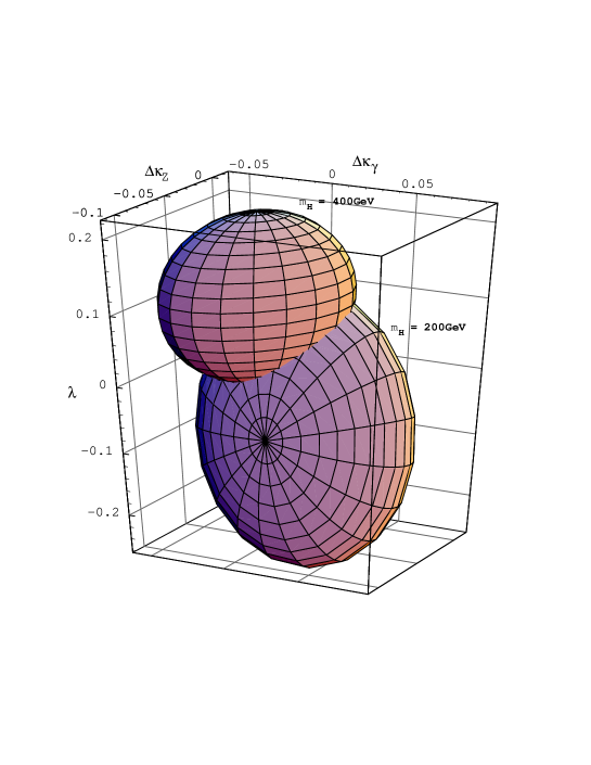
FIG. 5.: Constraints on $\Delta\kappa_{\gamma}$, $\Delta\kappa_{Z}$ and $\lambda=\lambda_{\gamma}=\lambda_{Z}$ at the 95% confidence level assuming the relations of Eqns. V with $\Lambda=$ 1 TeV and $m_{t}=$ 175 GeV.

Both contours are consistent with the SM, though the $m_{H}=$ 200 GeV contour just barely includes the SM value of $\lambda=0$. For $m_{H}=$ 200 GeV we observe a strong $\Delta\kappa_{Z}$–$\lambda$ correlation which is important when considering the measurement of these couplings at the Fermilab Tevatron. The Tevatron is sensitive to the $WW\gamma$ vertex primarily through the observation of $W\gamma$ pairs, but due to a limited center-of-mass energy $WW$ and $WZ$ events are rare. Therefore, at the Tevatron we are primarily interested in a two-dimensional plot in the $\Delta\kappa_{\gamma}$–$\lambda$ plane with a fixed value of $\Delta\kappa_{Z}$. Fig. 6(a) is a fit in the $\Delta\kappa_{\gamma}$–$\lambda$ plane for $m_{H}=$ 200 GeV, and Fig. 6(b) is the same plot for $m_{H}=$ 400 GeV. The solid, dashed and dotted contours correspond to $\Delta\kappa_{Z}=0$, $-0.1$ and $0.1$ respectively.

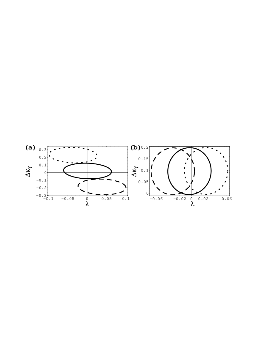
FIG. 6.: Constraints in the $\Delta\kappa_{\gamma}$–$\lambda$ plane at the 95% confidence level assuming the relations of Eqns. V with $\Lambda=$ 1 TeV and $m_{t}=$ 175 GeV. Fig. 6(a) corresponds to $m_{H}=$ 200 GeV while Fig. 6(b) corresponds to $m_{H}=$ 400 GeV. The solid, dashed and dotted contours correspond to $\Delta\kappa_{Z}=0$, $-0.1$ and $0.1$ respectively.

Notice that the $m_{H}=$ 200 GeV contour with $\Delta\kappa_{Z}=0$ is very consistent with the SM while all of the $m_{H}=$ 400 GeV contours barely cross the $\lambda=0$ axis. Clearly there is much more sensitivity to the assumed value of $\Delta\kappa_{Z}$ when the Higgs boson is light.

B Results for the nonlinear model

In order to perform the fits in the nonlinear case we calculate the SM values using $m_{H}=1$ TeV. Correspondingly we take $\hat{\mu}=1$ TeV in Eqns. (57) and (60), effectively subtracting off the Higgs-boson contributions. This method of subtracting off the SM Higgs-boson contributions is approximate, and in principle we should also subtract off all of the small finite $m_{H}$-dependent terms, or we should repeat the calculation of the higher-order effects excluding the Higgs boson from the beginning. The nonzero expressions for $R_{\gamma\gamma}$, $R_{\gamma Z}$, $R_{ZZ}$ and $R_{WW}$ in Eqns. (* ‣ IV) is a clear signal that the one-loop calculations including ${\cal O}(E^{4})\,$operators have induced ${\cal O}(E^{6})\,$effects. Therefore, to be completely consistent through ${\cal O}(E^{6})\,$, we should add to Eqns. (* ‣ IV) the two-loop contributions of the ${\cal O}(E^{2})\,$operator ${\cal L}_{1}^{\prime}$ and the tree-level contributions of a complete set of ${\cal O}(E^{6})\,$chiral operators. Excluding these effects is an approximation, and in order to proceed we must assume that the excluded effects do not significantly interfere with the contributions of ${\cal L}_{1}^{\prime}$-${\cal L}_{10}$.

First we analyze the numerical constraints on $\alpha_{1}$, $\beta_{1}$ and $\alpha_{8}$ (which correspond to $\Delta S$, $\Delta T$ and $\Delta U$, respectively), and we present the best-fit central values with one-sigma errors,

$$\left.\begin{array}[]{lll}\alpha_{1}&=&(4.7\pm 2.6)\times 10^{-3}\;,\\ \beta_{1}&=&(0.30\pm 0.57)\times 10^{-3}\;,\\ \alpha_{8}&=&(-0.9\pm 7.6)\times 10^{-3}\;,\end{array}\right.$$ (92)

and the full correlation matrix,

$$\rho_{\rm corr}=\left(\makebox[-8.5359pt]{}\begin{array}[]{ldd}\hbox to15.00005pt{\hss 1}\hbox to15.00005pt{\hfill}&\hbox to15.00005pt{\hss$-$0}\hbox to15.00005pt{.871\hss}$&\hbox to15.00005pt{\hss$-$0}\hbox to15.00005pt{.121\hss}$\\ &\hbox to15.00005pt{\hss 1}\hbox to15.00005pt{\hfill}$&\hbox to15.00005pt{\hss 0}\hbox to15.00005pt{.221\hss}$\\ &$&\hbox to15.00005pt{\hss 1}\hbox to15.00005pt{\hfill}$\end{array}\right)\;.$$ (93)

These tree-level contributions are nondecoupling effects, hence the bounds derived are insensitive to the scale $\Lambda$. These constraints are sufficiently strong that there is no sensitivity to these three parameters at LEP II[16, 18]. Observe that a positive value for $\alpha_{1}$ is favored. If we insist that either $\alpha_{1}=0$ or $\beta_{1}=0$, then the $\alpha_{1}$–$\beta_{1}$ anti-correlation forces the other parameter towards a more positive central value. Accordingly, in Table II, we present the 95% confidence-level limits where only one of $\alpha_{1}$, $\beta_{1}$ or $\alpha_{8}$ is allowed to deviate from zero.

$\beta_{1}$	$\alpha_{1}$	$\alpha_{8}$
(1.2$\pm$1.0)$\times 10^{-3}$	(6.0$\pm$4.9)$\times 10^{-3}$	(-7$\pm$28)$\times 10^{-3}$

TABLE II.: 95% confidence-level constraints on $\beta_{1}$, $\alpha_{1}$ and $\alpha_{8}$ for $m_{t}=175$ GeV. These results are independent of $\Lambda$. In this table only one coupling at a time is allowed to deviate from zero.

Indeed we see that a more positive value for both $\alpha_{1}$ and $\beta_{1}$ is preferred, and the fitted value of $\beta_{1}$ now deviates significantly from the SM.

Next we place constraints on the remaining parameters by considering the effects of only one operator at a time. The results are summarized in Table III.

	$\alpha_{2}$	$\alpha_{3}$	$\alpha_{9}$	$\frac{2}{5}\alpha_{4}+\alpha_{5}+14.9\alpha_{6}+15.6\alpha_{7}+14.7\alpha_{10}$
$\alpha_{1}=0$	0.25$\pm$0.20	-0.12$\pm$0.09	-0.27$\pm$0.61	-0.44$\pm$0.35
$\alpha_{1}=5.5\times 10^{-3}$	0.03$\pm$0.20	-0.05$\pm$0.09	-0.28$\pm$0.61	-0.09$\pm$0.37

TABLE III.: 95% confidence-level constraints on $\alpha_{2}$–$\alpha_{7}$, $\alpha_{9}$ and $\alpha_{10}$ for $m_{t}=175$ GeV and $\Lambda=1$ TeV. Only the linear combination of $\alpha_{4}$–$\alpha_{7}$ and $\alpha_{10}$ shown in the last column may be constrained. In the first row all other coefficients are set to zero. In the second row $\alpha_{1}=5.5\times 10^{-3}$ is chosen according to Eqn.(92).

First of all, notice that $\alpha_{4}$–$\alpha_{7}$ and $\alpha_{10}$ enter into the analysis only through their contribution to $\Delta T$ as shown in Eqn. (60), hence only the linear combination of these five coefficients shown in the last column may be constrained. Furthermore, $\alpha_{1}$ is anticorrelated with this linear combination in the same fashion as with $\beta_{1}$. Notice that in the first row of the table, when $\alpha_{1}=0$, only $\alpha_{9}$ is consistent with SM at the 95% confidence level. However, in the second row where we have chosen the central value of $\alpha_{1}$ according to the best-fit value of Eqn. (92), all of the central values are easily consistent with the zero. While the central values easily move around as we include additional operators in the analysis, the errors are much more robust.

Three of the coefficients, $\alpha_{2}$, $\alpha_{3}$ and $\alpha_{9}$, contribute at the tree-level to nonstandard $WW\gamma$ and $WWZ$ vertices without making a tree-level contribution to low-energy and Z-pole observables. In Fig. 7(a) we plot 95% confidence-level limits obtained

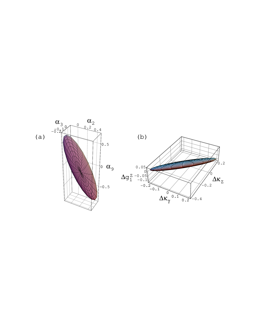
FIG. 7.: 95% confidence level contours for $\Lambda=$ 1 TeV and $m_{t}=$ 175 GeV. In (a) we show the fit in $\alpha_{2}$, $\alpha_{3}$ and $\alpha_{9}$. In (b) we have reparameterized the fit in terms of $\Delta\kappa_{\gamma}$, $\Delta\kappa_{Z}$ and $\Delta g_{1}^{Z}$ according to the relations of Eqns. (V).

by fitting $\alpha_{2}$, $\alpha_{3}$ and $\alpha_{9}$. There is a very strong $\alpha_{2}$–$\alpha_{3}$ correlation and moderately strong $\alpha_{2}$–$\alpha_{9}$ and $\alpha_{3}$–$\alpha_{9}$ anti-correlations. Then, using Eqns. (V), we may recast the fit in terms of $\Delta\kappa_{\gamma}$, $\Delta\kappa_{Z}$ and $\Delta g_{1}^{Z}$. The results are displayed in Fig. 7(b). In this basis the correlations are not as strong; there are moderately strong $\Delta\kappa_{\gamma}$–$\Delta\kappa_{Z}$ and $\Delta\kappa_{\gamma}$–$\Delta g_{1}^{Z}$ correlations. In Fig. 7(a) the point $\alpha_{3}=0$ (equivalently, in Fig. 7(b), the point $\Delta g_{1}^{Z}=0$) lies near the edge of the contour.

If we require any new physics to conserve the SU(2)_C symmetry, then $\alpha_{9}=0$. In this case there are only two free parameters, $\alpha_{2}$ and $\alpha_{3}$; equivalently we can choose any two parameters from the set $\{\Delta\kappa_{\gamma},\Delta\kappa_{Z},\Delta g_{1}^{Z}\}$, and once again we use the relations of Eqns. (V). Recalling that $\alpha_{2}$ and $\alpha_{3}$ are related to $f_{B}$ and $f_{W}$ by Eqns. (IV) we can perform the analogous fit in the linear realization of SSB which is shown in Fig. 8.

FIG. 8.: 95% confidence level contours for $\Lambda=$ 1 TeV and $m_{t}=$ 175 GeV. The solid, dashed and dotted curves correspond to $m_{H}=100$ GeV, $m_{H}=300$ GeV and $m_{H}=700$ GeV; these first three curves use Eqns. (V). The dot-dashed curve corresponds to the nonlinear realization of SSB and therefore employs Eqns. (V).

The solid, dashed and dotted curves correspond to $m_{H}=100$ GeV, $m_{H}=300$ GeV and $m_{H}=700$ GeV; these first three curves use Eqns. (V). The $m_{H}=100$ GeV is very consistent with the SM while the $m_{H}=300$ GeV and $m_{H}=700$ GeV contours prefer nonzero values for $\Delta\kappa_{Z}$; the centers and the orientations of these ellipses are complicated functions of $m_{H}$, but the contours clearly become smaller with increasing Higgs-boson mass. The dot-dashed curve corresponds to the nonlinear realization of SSB and therefore employs Eqns. (V). It clearly does not include the SM, but its center could be shifted by including nonzero central values for $\alpha_{1}$ and $\beta_{1}$ according to Eqn. (92).

In any realistic scenario there will be a set of nonzero $\alpha_{i}$, and it is possible (indeed likely) that there will be large interference between the effects of the various coefficients. In order to see the types of limits which might arise in various scenarios of SSB we consider a strongly interacting scalar and a degenerate doublet of heavy fermions, and we get an indication of the sensitivity of our results to the underlying dynamics. Using the effective-Lagrangian approach, we can estimate the coefficients in a consistent way.

We first consider a model with three Goldstone bosons corresponding to the longitudinal components of the $W^{\pm}$ and $Z$ and bosons coupled to a scalar isoscalar resonance like the Higgs boson. We assume that the $\alpha_{i}(\mu^{2})$ are dominated by tree-level exchange of the scalar boson. Integrating out the scalar and matching the coefficients at the scale $m_{H}$ gives the predictions[6, 36, 37],

$$\alpha_{4}(\mu^{2}) = \frac{1}{16\pi^{2}}\frac{1}{12}\log\bigg{(}\frac{m_{H}^{2}}{\mu^{2}}\bigg{)}$$ (95)

$$= 2\alpha_{2}(\mu^{2})=2\alpha_{3}(\mu^{2})=-\alpha_{1}(\mu^{2})$$ (96)

$$\alpha_{5}(\mu^{2}) = \frac{1}{16\pi^{2}}\Bigg{[}\frac{1}{24}\log\bigg{(}\frac{m_{H}^{2}}{\mu^{2}}\bigg{)}+\frac{64\pi^{3}}{3}\frac{\Gamma_{h}v^{4}}{m_{H}^{5}}\Bigg{]},$$ (97)

where $\Gamma_{h}$ is the width of the scalar into Goldstone bosons. All of the other $\alpha_{i}$ are zero in this scenario. It is important to note that only the logarithmic terms are uniquely specified. The constant terms depend on the renormalization scheme[37, 38]. (We use the renormalization scheme of Ref. [38].)

In Fig. 9

FIG. 9.: 95% confidence level contours for $\Lambda=$ 1 TeV and $m_{t}=$ 175 GeV in the $\alpha_{5}$–$\alpha_{1}$ plane subject to $-\alpha_{1}(\mu^{2})=2\alpha_{2}(\mu^{2})=2\alpha_{3}(\mu^{2})=\alpha_{4}(\mu^{2})$. The larger (smaller) contour corresponds to $\mu=500$ GeV ($\mu=m_{Z}$).

we plot $\alpha_{5}(\mu^{2})$ vs. $\alpha_{1}(\mu^{2})$ with the pattern typical of a theory dominated by a heavy scalar given in Eqn. (8), $-\alpha_{1}(\mu^{2})=2\alpha_{2}(\mu^{2})=2\alpha_{3}(\mu^{2})=\alpha_{4}(\mu^{2})$. First of all, notice that the contour obtained depends rather strongly upon our choice of the renormalization scale, $\mu$, especially with regard to the $\alpha_{5}$ axis. Everything to the right of $\alpha_{1}=0$ corresponds to $m_{H}<\mu$. Furthermore, since we require that $\Gamma_{h}$ be non-negative, we may approximately exclude everything below the $\alpha_{5}=0$ axis. The allowed region to the upper right of the figure corresponds to a Higgs-boson with a mass in the MeV range and an extremely narrow width; this portion of the figure is already excluded by experiment. An approximate upper bound on $m_{H}$ can be obtained from the leftmost point where both curves intersect the horizontal axis; as this figure is drawn the entire plane is excluded by LEP. We can, by changing $\Lambda$ and $\mu$, drive the upper bound above 100 GeV or greater, but the positive central value of $\alpha_{1}$ indicates that a heavy scalar resonance is disfavored.

The previous example conserves the custodial SU(2)_C symmetry. The simplest example of dynamics which violates the custodial symmetry is a heavy doublet of nondegenerate fermions. Ref. [24] considers the case of a heavy doublet with charge $\pm\frac{1}{2}$, a mass splitting $\Delta m$, and an average mass $M$ with ($\Delta m\ll M$). Then assuming the fermions are in a color triplet and retaining terms to ${\cal O}(\delta^{2})$, ($\delta\equiv{\Delta m\over 2M}$), they find

$$\beta_{1}(m_{Z}^{2}) = \frac{1}{8\pi^{2}}\frac{(\Delta m)^{2}}{m_{W}^{2}}\;,$$ (99)

$$\alpha_{1}(m_{Z}^{2}) = \alpha_{2}(m_{Z}^{2})=-\frac{1}{32\pi^{2}}\;,$$ (100)

$$\alpha_{3}(m_{Z}^{2}) = -\frac{1}{32\pi^{2}}\bigg{(}1-\frac{2}{5}\delta^{2}\bigg{)}\;,$$ (101)

$$\alpha_{8}(m_{Z}^{2}) = -\frac{1}{32\pi^{2}}\frac{16}{5}\delta^{2}\;,$$ (102)

$$\alpha_{9}(m_{Z}^{2}) = -\frac{1}{32\pi^{2}}\frac{14}{5}\delta^{2}\;,$$ (103)

$$\alpha_{11}(m_{Z}^{2}) = \frac{1}{32\pi^{2}}\delta\;,$$ (104)

Because of the heavy fermion masses in the loops, the $\alpha_{i}$ are finite and there are no logarithms of $\Lambda$ in Eqns. (9). The custodial SU(2)_C violation can be clearly seen in the terms proportional to $\delta$. As in the case of the heavy Higgs boson, we note that the coefficients are naturally ${\cal O}(1/16\pi^{2})$. (For a discussion where the mass splitting is arbitrary, see Ref. [39].)

This model generates a nonzero value for $\alpha_{11}$, but we have not included $\alpha_{11}$ in our analysis. This is not a problem since we expect the analysis to be dominated by the tree-level contributions of $\beta_{1}$, $\alpha_{1}$ and $\alpha_{8}$; we will neglect the contributions of the other coefficients. In Fig. 10 we show the 95% confidence-level limits in the $(\Delta m)^{2}$–$\delta^{2}$ plane.

FIG. 10.: 95% confidence level contours for in the $(\Delta m)^{2}$–$\delta^{2}$ using the parameters of Eqn. 9. Numerically there is an allowed region for $\delta^{2}<0$. However, $\delta^{2}<0$ is unphysical, and we do not show it. All numbers are in GeV².

We have excluded the unphysical $\delta^{2}<0$ portion of the ellipse. However, the calculation is not valid for a portion of the region shown. We have explicitly assumed that $\Delta m\ll M$. If we choose a very loose cut-off of $\Delta m<0.4M$, then we should restrict the figure to $\delta^{2}<0.04$, and only a narrow strip along the bottom of the figure is relevant. For $\delta^{2}=0$, $M\rightarrow\infty$, and we cannot obtain an upper bound on $M$. We cannot obtain a lower bound on $M$ because the contour extends into a region where our calculation is not valid. If we insist that the new fermions are heavier than approximately 200 GeV, then $\Delta M\sim{\cal O}(60-90~{}{\rm GeV})$ is the preferred region for the mass splitting.

VII Conclusions

Parameterizing the contributions of new physics at low energies with an effective Lagrangian we have studied the contributions of new physics to electroweak observables; everywhere we have treated the linear and nonlinear realizations of electroweak symmetry breaking in parallel, allowing us to make direct comparisons which had not previously been studied. The complete contributions of the new physics to low-energy and Z-pole observables may be completely summarised by expressions for the running charges $\overline{\alpha}(q^{2})$, $\overline{g}_{Z}^{2}(q^{2})$, $\overline{s}^{2}(q^{2})$ and $\overline{g}_{W}^{2}(q^{2})$ plus a form factor for the $Zbb$ vertex, $\overline{\delta}_{b}(q^{2})$. We present explicit expressions for these quantities in both realizations of symmetry breaking.

The above approach is ideally suited to performing a global analysis using all available electroweak precision data. We perform many such fits. We study the bounds which may be obtained on the various effective-Lagrangian parameters and the bounds on nonstandard $WW\gamma$ and $WWZ$ couplings. For the case of nonstandard $WW\gamma$ and $WWZ$ couplings we are able to investigate the role of the Higgs mass as compared to having no Higgs boson as all. See Fig. 8.

The coefficients of some operators in the effective Lagrangian contribute to four-fermion amplitudes at the tree level while the coefficients of others first contribute at the loop level. A topic of great interest is whether the former can be suppressed relative to the latter. We discuss one toy model where such a hierarchy is realized. If such a hierarchy could be realized among the operators that contribute to $WW\gamma$ and $WWZ$ couplings, then, even allowing for some correlations, the low-energy bounds are in some cases on par with or even superior to the bounds that can be obtained at LEP II.

We then use our global analysis to examine some explicit models. For the case of a strongly interacting model with a scalar Higgs boson, a light scalar is strongly prefered, while much of the light region has already been ruled out by LEP. We confirm that a positive value for $\alpha_{1}$ is prefered, which is known to strongly disfavor the simplest models that include a strongly interacting vector-like Higgs boson. Finally we consider the contributions of a heavy pair of new fermions. While our analysis is only valid if their masses are heavier than 200-300 GeV, we find that a mass splitting of 60-90 GeV is prefered.

A Operators in the linear realization of SSB

In this appendix we explicitly enumerate the operators of Eqn. (30), i.e. the effective Lagrangian with the linear realization of SSB. The twelve operators discussed in Section III are

$${\cal O}_{DW} = -\hat{g}^{2}{\rm Tr}\bigg{[}\Big{(}\partial_{\mu}W_{\nu\rho}\Big{)}\Big{(}\partial^{\mu}W^{\nu\rho}\Big{)}\bigg{]}\;,$$ (A2)

$${\cal O}_{DB} = -\frac{\hat{g}^{\prime\;2}}{2}\Big{(}\partial_{\mu}B_{\nu\rho}\Big{)}\Big{(}\partial^{\mu}B^{\nu\rho}\Big{)}\;,$$ (A3)

$${\cal O}_{BW} = -\frac{\hat{g}\hat{g}^{\prime}}{2}\Phi^{\dagger}B_{\mu\nu}W^{\mu\nu}\Phi\;,$$ (A4)

$${\cal O}_{\Phi,1} = \bigg{[}\Big{(}D_{\mu}\Phi\Big{)}^{\dagger}\Phi\bigg{]}\;\bigg{[}\Phi^{\dagger}\Big{(}D^{\mu}\Phi\Big{)}\bigg{]}\;,$$ (A5)

$${\cal O}_{WWW} = -i\frac{3}{2}\hat{g}^{3}W^{+}_{\mu\nu}W^{-\;\nu\rho}W^{3\;\mu}_{\rho}\;,$$ (A6)

$${\cal O}_{W} = i\hat{g}\Big{(}D_{\mu}\Phi\Big{)}^{\dagger}W^{\mu\nu}\Big{(}D_{\nu}\Phi\Big{)}\;,$$ (A7)

$${\cal O}_{B} = \frac{i}{2}\hat{g}^{\prime}\Big{(}D_{\mu}\Phi\Big{)}^{\dagger}B^{\mu\nu}\Big{(}D_{\nu}\Phi\Big{)}\;,$$ (A8)

$${\cal O}_{WW} = -\frac{\hat{g}^{2}}{4}\Big{(}\Phi^{\dagger}\Phi\Big{)}W^{I\,\mu\nu}W^{I}_{\mu\nu}\;,$$ (A9)

$${\cal O}_{BB} = -\frac{\hat{g}^{\prime\,2}}{4}\Big{(}\Phi^{\dagger}\Phi\Big{)}B^{\mu\nu}B_{\mu\nu}\;,$$ (A10)

$${\cal O}_{\Phi,2} = \frac{1}{2}\partial_{\mu}\Big{(}\Phi^{\dagger}\Phi\Big{)}\partial^{\mu}\Big{(}\Phi^{\dagger}\Phi\Big{)}\;,$$ (A11)

$${\cal O}_{\Phi,3} = \frac{1}{3}\Big{(}\Phi^{\dagger}\Phi\Big{)}^{3}\;,$$ (A12)

$${\cal O}_{\Phi,4} = \Big{(}\Phi^{\dagger}\Phi\Big{)}\bigg{[}\Big{(}D_{\mu}\Phi\Big{)}^{\dagger}\Big{(}D^{\mu}\Phi\Big{)}\bigg{]}\;,$$ (A13)

where $W_{\mu\nu}=T^{a}W^{a}_{\mu\nu}$. The field strength tensors are given by

$$B_{\mu\nu} = \partial_{\mu}B_{\nu}-\partial_{\nu}B_{\mu}\;,$$ (A15)

$$W_{\mu\nu} = \partial_{\mu}W_{\nu}-\partial_{\nu}W_{\mu}-g\epsilon_{abc}W_{\mu}^{b}W_{\nu}^{c}\;,$$ (A16)

where $\epsilon_{abc}$ is the totally antisymmetric tensor in three dimensions with $\epsilon_{123}=1$. The covariant derivative is given by

$$D_{\mu}=\partial_{\mu}+igT^{a}W^{a}_{\mu}+ig^{\prime}YB_{\mu},$$ (A17)

and $\Phi$ is the SM Higgs doublet,

$$\Phi=\frac{1}{\sqrt{2}}\left(\begin{array}[]{c}i\chi^{1}+\chi^{2}\\ v+H-i\chi^{3}\end{array}\right)\;.$$ (A18)

B Operators in the electroweak chiral Lagrangian

In this appendix we present explicitly the operators of the electroweak chiral Lagrangian. In the notation of Ref. [22, 23, 24],

$${\cal L}_{\rm eff}^{\rm nlr}={\cal L}_{\rm SM}^{\rm nlr}+\sum{\cal L}_{i}+\cdots\;.$$ (B1)

We use the superscript ‘nlr’, denoting ‘nonlinear realization’. The first term is the SM Lagrangian, but in this case no physical Higgs boson is included. Hence ${\cal L}_{\rm SM}^{\rm nlr}$ is nonrenormalizable. The first non-SM terms are energy dimension-two and -four operators which are not manifestly suppressed by explicit powers of some high scale.

While the physical Higgs boson has not been employed, the Goldstone bosons, $\chi_{i}$ for $i=1,2,3$, are included through the unitary unimodular field $U$ introduced below. Following Ref. [24],

$$U \equiv \exp\bigg{(}\frac{2i\,\chi_{i}(x)\tau_{i}}{v}\bigg{)}\longrightarrow{\bf 1}\;,$$ (B3)

$$D_{\mu}U \equiv \partial_{\mu}U+igT^{a}W_{\mu}^{a}U-ig^{\prime}UT^{3}B_{\mu}\longrightarrow igT^{a}W_{\mu}^{a}-ig^{\prime}T^{3}B_{\mu}\;,$$ (B4)

$$T \equiv 2UT^{3}U^{\dagger}\longrightarrow 2T^{3}\;,$$ (B5)

$$V_{\mu} \equiv (D_{\mu}U)U^{\dagger}\longrightarrow D_{\mu}U\;,$$ (B6)

where $\bf 1$ is the 2$\times$2 identity matrix, the Pauli matrices are denoted by $\tau_{i}$, and $T_{i}=\tau_{i}/2$ with the normalization Tr$(T_{i}T_{j})=\frac{1}{2}\delta_{ij}$. The right-pointing arrow indicates the unitary-gauge form of each expression. The lowest order effective Lagrangian for the symmetry breaking sector of the theory is

$${\cal L}_{SM}={v^{2}\over 4}Tr\biggl{[}D_{\mu}U^{\dagger}D^{\mu}U\biggr{]}\quad.$$ (B7)

The non-SM operators with four or fewer derivatives which conserve CP are[23, 24],

$${\cal L}_{1}^{\prime} = \frac{1}{4}\beta_{1}v^{2}\Big{[}{\rm Tr}(TV_{\mu})\Big{]}^{2}\;,$$ (B9)

$${\cal L}_{1} = \frac{1}{2}\alpha_{1}\hat{g}\hat{g}^{\prime}{\rm Tr}\Big{(}B_{\mu\nu}TW^{\mu\nu}\Big{)}\;,$$ (B10)

$${\cal L}_{2} = \frac{i}{2}\alpha_{2}\hat{g}^{\prime}B_{\mu\nu}{\rm Tr}\Big{(}T[V^{\mu},V^{\nu}]\Big{)}\;,$$ (B11)

$${\cal L}_{3} = i\alpha_{3}\hat{g}{\rm Tr}\Big{(}W_{\mu\nu}[V^{\mu},V^{\nu}]\Big{)}\;,$$ (B12)

$${\cal L}_{4} = \alpha_{4}\Big{[}{\rm Tr}(V_{\mu}V_{\nu})\Big{]}^{2}\;,$$ (B13)

$${\cal L}_{5} = \alpha_{5}\Big{[}{\rm Tr}(V_{\mu}V^{\mu})\Big{]}^{2}\;,$$ (B14)

$${\cal L}_{6} = \alpha_{6}{\rm Tr}\Big{(}V_{\mu}V_{\nu}\Big{)}{\rm Tr}\Big{(}TV^{\mu}\Big{)}{\rm Tr}\Big{(}TV^{\nu}\Big{)}\;,$$ (B15)

$${\cal L}_{7} = \alpha_{7}{\rm Tr}\Big{(}V_{\mu}V^{\mu}\Big{)}{\rm Tr}\Big{(}TV_{\nu}\Big{)}{\rm Tr}\Big{(}TV^{\nu}\Big{)}\;,$$ (B16)

$${\cal L}_{8} = \frac{1}{4}\alpha_{8}\hat{g}^{2}\Big{[}{\rm Tr}(TW_{\mu\nu})\Big{]}^{2}\;,$$ (B17)

$${\cal L}_{9} = \frac{i}{2}\alpha_{9}\hat{g}{\rm Tr}\Big{(}TW_{\mu\nu}\Big{)}{\rm Tr}\Big{(}T[V^{\mu},V^{\nu}]\Big{)}\;,$$ (B18)

$${\cal L}_{10} = \frac{1}{2}\alpha_{10}\Big{[}{\rm Tr}(TV_{\mu}){\rm Tr}(TV_{\nu})\Big{]}^{2}\;,$$ (B19)

$${\cal L}_{11} = \alpha_{11}\hat{g}\,\epsilon^{\mu\nu\rho\sigma}{\rm Tr}\Big{(}TV_{\mu}\Big{)}{\rm Tr}\Big{(}V_{\nu}W_{\rho\sigma}\Big{)}\;.$$ (B20)

REFERENCES

- [1] K. Hagiwara, D. Haidt, C. S. Kim and S. Matsumoto, Z. Phys. C64 (1994) 559.
- [2] D.C. Kennedy and B.W. Lynn, Nucl. Phys. B322 (1989) 1.
- [3] J.M. Cornwall and J. Papavassiliou, Phys. Rev. D40 (1989) 3474; J. Papavassiliou, Phys. Rev. D41 (1990) 3179.
- [4] G. Degrassi and A. Sirlin, Nucl. Phys. B383 (1992) 73; Phys. Rev. D46 (1992) 3104; G. Degrassi, B.A. Kniehl and A. Sirlin, Phys. Rev. D48 (1993) 3963.
- [5] J. Papavassiliou and K. Philippides, Phys. Rev. D48 (1993) 4255; J. Papavassiliou and A. Sirlin, Phys. Rev. D50 (1994) 5951; J. Papavassiliou, Phys. Rev. D50 (1994) 5958; J. Papavassiliou and K. Philippides, Phys. Rev. D52 (1995) 2355; J. Papavassiliou, (Feb. 1995) hep-ph-9504382; J. Papavassiliou and A. Pilaftsis, Phys. Rev. Lett. 75 (1995) 3060.
- [6] T. Appelquist and C. Bernard, Phys. Rev. D22 (1980) 200.
- [7] K. Hagiwara, S. Ishihara, R. Szalapski and D. Zeppenfeld, Phys. Rev. D48 (1993) 2182.
- [8] M.E. Peskin and T. Takeuchi, Phys. Rev. Lett. 65 (1990) 964; Phys. Rev. D46 (1992) 381.
- [9] G. Altarelli and R. Barbieri, Phys. Lett. B253 (1991) 161; G. Altarelli, R. Barbieri and S. Jadach, Nucl. Phys. B369 (1992) 3; W.J. Marciano and J.L. Rosner, Phys. Rev. Lett. 65 (1990) 2963; D.C. Kennedy and P. Langacker, Phys. Rev. Lett. 65 (1990) 2967; D.C. Kennedy and P. Langacker, Phys. Rev. D44 (1991) 1591.
- [10] C.P. Burgess, David London, I. Maksymyk, Phys. Rev. D50 (1994) 529; C.P. Burgess, Stephen Godfrey, Heinz Konig, David London, I. Maksymyk, Phys. Lett. B326 (1994) 276. C.P. Burgess, hep-ph/9411257 (1994).
- [11] J. Papavassiliou, E. de Rafael, N.J. Watson, CPT-96-P-3408, hep-ph/9612237.
- [12] W. Buchmüller and D. Wyler, Nucl. Phys. B268 621 (1986).
- [13] C. J. C. Burgess and H. J. Schnitzer, Nucl. Phys. B228, 464 (1983); C. N. Leung, S. T. Love, and S. Rao, Z. Phys. C31, 433 (1986).
- [14] K. Hagiwara, S. Ishihara, R. Szalapski and D. Zeppenfeld, Phys. Lett. B283 (1992) 353; K. Hagiwara, S. Ishihara, R. Szalapski and D. Zeppenfeld, Phys. Rev. D48 (1993) 2182.
- [15] B. Grinstein and M.B. Wise, Phys. Lett. B265 (1991) 326.
- [16] K. Hagiwara, S. Matsumoto and R. Szalapski, Phys. Lett. B357 (1995) 411.
- [17] K. Hagiwara, R. Szalapski and D. Zeppenfeld, Phys. Lett. B318 (1993) 155-162; G.J. Gounaris, F.M. Renard, N.D. Vlachos, Nucl. Phys. B459 (1996) 51-74; G.J. Gounaris, F.M. Renard, Z. Phys. C69 (1996) 513-518.
- [18] K. Hagiwara, T. Hatsukano, S. Ishihara and R. Szalapski, To be published in Nucl. Phys. B. KEK-TH-497, hep-ph/9612268.
- [19] A. De Rújula, M.B. Gavela, P. Hernandez and E. Massó, Nucl. Phys. B384 (1992) 3.
- [20] S. Dawson and G. Valencia, Nucl. Phys. B439 (1995) 3-22.
- [21] C.P. Burgess, S. Godfrey, H. Konig, D. London, I. Maksymyk, Phys. Rev. D49 (1994) 6115-6147.
- [22] A.C. Longhitano, Phys. Rev. D22 (1980) 1166.
- [23] A.C. Longhitano, Nucl. Phys. B188 (1981) 118.
- [24] T. Appelquist and G.H. Wu, Phys. Rev. D48 (1993) 3235.
- [25] S. Dawson and G. Valencia, Phys. Lett. B333 (1994) 207-211.
- [26] Talk by K. Hagiwara at The International Symposium on Vector Boson Self Interactions, UCLA, Feb. 1-3, 1995, KEK-TH-442.
- [27] A. Brunstein, O.J.P. Eboli, M.C. Gonzalez-Garcia, Phys. Lett. B375 (1996) 233-239.
- [28] A. Dobbado, D. Espriu, and M. Herrero, Phys. Lett. B255 (1991) 405.
- [29] K. Hagiwara, R.D. Peccei, D. Zeppenfeld and K. Hikasa, Nucl. Phys. B282 (1987) 253; T. Barklow, U. Baur, et. al., Proceedings 1996 DPF/DPB Snowmass Workshop, Snowmass, Colorado, 1996, hep-ph/9611454.
- [30] F. Feruglio, Int. Journ. of Mod. Phys. A8 (1993) 4937.
- [31] K. Hagiwara, D. Haidt and S. Matsumoto, KEK-TH-512, DESY 96-192, hep-ph/9706331, for publication in Z. Phys. C.
- [32] Particle Data Group, R.M. Barnett et al., Phys. Rev. D54 (1996) 1-720.
- [33] D. Donjerkovic and D. Zeppenfeld, private communication.
- [34] S. Dawson, A. Likhoded, G. Valencia, O. Yushchenko et. al., Proceedings 1996 DPF/DPB Snowmass Workshop, Snowmass, Colorado, 1996, hep-ph/9610299.
- [35] F. Boudjema, Proceedings of 3rd Workshop on Physics and Experiments with Linear Colliders, Iwate, Japan, Sept. 1995, hep-ph/9701409.
- [36] J. Donoghue, C. Ramirez, and G. Valencia, Phys. Rev. D39 (1989) 1947.
- [37] M. Herrero and E. Morales, Nucl. Phys. B437 (1995) 319.
- [38] J. Bagger, S. Dawson, and G. Valencia, Nucl. Phys. B399 (1993) 364.
- [39] F. Feruglio, A. Masiero, S. Rigolin and R. Strocchi, Phys. Lett. B355 (1995) 329.