Abstract

We study the various stages of the evolution of chiral condensates disoriented via the “baked-alaska” mechanism, in which the condensates are described as the products of external sources localized on the light cone. Our analysis is based on the classical equations of motion of either the linear or the nonlinear sigma model. We use the associated framework of coherent states and, especially, their source functions to make the connection to the distribution functions for the produced particles. We also compare our classical approach with a mean-field calculation which includes a certain class of quantum corrections.

Submitted to Physical Review D.

1 Introduction

Recently, in order to interpret events with a deficit or excess of neutral pions observed in cosmic ray experiments, there has been increased interest in the conjecture that it might be possible to produce in high-energy collisions disoriented chiral condensates (DCCs), i.e. correlated regions of space-time wherein the quark condensate, $\langle 0|q_{L}\bar{q}_{R}|0\rangle$, is chirally rotated from its usual orientation in isospin space.

On the theoretical side there has been great interest (see, e.g., Refs. [1]-[14]) both in the development of technical tools suitable for the description of this possible phenomenon, and in the exploration of the possibilities opened by DCCs as probes of the structure of quantum chromodynamics, most notably in relation to the chiral phase transition.

The idea that such DCCs might be produced in high energy collisions at existing or planned hadron or heavy-ion accelerators has generated some experimental interest. In particular, one of us is co-spokesman for a Fermilab experiment [15] looking for DCCs in hadron-hadron collisions. In high energy $p$-${\bar{p}}$ collisions which lead to a sizable multiplicity of produced particles, but not necessarily with high-$p_{T}$ jets in the final state, the time evolution is quasi-macroscopic, because the hadronization time can be rather large, up to 3-5 $fm$. At times $t$ before hadronization, the initial state partons, produced in a volume much smaller than a cubic fermi, may stream outward at essentially the speed of light in all directions, occupying the surface of a sphere of radius $t$ (in units such that the speed of light is 1). Most of the outgoing energy/momentum is expected to be concentrated near the light cone, i.e. on the surface of the expanding ‘fireball’.

However, the interior of the fireball is also an interesting place. If its energy density is low enough, the interior should look very similar to the vacuum, with an associated non-vanishing quark condensate. Since the energy density from the intrinsic chiral symmetry breaking is small [6, 16], and since the fireball surface isolates the interior from the exterior of the light cone, it is reasonable to consider the possibility that well inside the light cone the quark condensate might be chirally rotated from its usual orientation. At late times this disoriented vacuum would relax back to ordinary vacuum, via radiation of its collective modes, the pions. The properties of the radiated pions should be strongly affected by the semiclassical, coherent nature of the process. In particular, one may expect anomalously large event-by-event fluctuations in the ratio of the number of charged pions to neutral pions produced. Assuming that the event-by-event deviation of the quark condensate from its usual orientation be random, one finds [1, 2, 3, 4, 16, 17] that the distribution $P(f)$ of the neutral fraction

$$f\equiv{N_{\pi^{0}}\over N_{\pi^{0}}+N_{\pi^{+}}+N_{\pi^{-}}}\equiv{N_{\pi^{0}}\over N_{tot}}~{},$$ (1)

is given by

$${dP\over df}={1\over 2\,\sqrt{f}}~{},$$ (2)

at large $N_{tot}$. Most notably, this implies that for “DCC pions” the probability of finding extreme values of $f$ is very different from ordinary pion production (which is given by a binomial distribution), in which the fluctuations are expected to be peaked at $f\!=\!1/3$ and fall exponentially away from the peak.

Experimental DCC searches [15] are thus far largely based on the structure of Eq. (2). However, it is probable that this robust property will not be sufficient on its own for the identification of phenomena involving DCCs. In particular, it appears that an understanding of the geometry of the phenomena would be very useful for experimental searches.

In this paper we develop a description of “baked-alaska” (hot fireball surface with cooler and disoriented inside) DCCs which is well suited for the study of realistic geometries. Our analysis is based on the classical equations of motion of either the linear or the nonlinear sigma model and we use the associated framework of coherent states to make the connection to the distribution functions for the produced particles.

In the next section we review the coherent-state formalism with emphasis on the associated particle flux, which is seen as directly related to classical sources localized on the light cone. Sec. 3 is devoted to the sigma model description of “baked-alaska DCCs”, defined via the above-mentioned mechanism involving a hot fireball shell and its cooler (and sometimes disoriented) interior. In Sec. 4 we derive a simple solution of the classical nonlinear sigma model, and follow the evolution of the associated coherent state from beginning to end, including a derivation of the flux of pions. In Sec. 5 we discuss how our analysis can be generalized to the linear sigma model, and establish connections with a somewhat similar model studied by Lampert, Dawson, and Cooper [18]. Sec. 6 is devoted to closing remarks.

2 Particle production from classical sources

2.1 Coherent state formalism

In the following sections we will be investigating a problem which in the classical limit is described by the field equation

$$(\Box+m^{2})\phi(x) = J(x)~{},$$ (3)

for appropriate boundary conditions. The properties of the quanta associated with a field, such as $\phi$ in (3), that are produced by a classical current source $J$ can be studied using the coherent state defined by

$$|J\rangle \equiv \exp\left[-{1\over 2}\int d\tilde{k}~{}|\tilde{J}(k)|^{2}\right]\exp\left[\int d\tilde{k}~{}\tilde{J}(k)\hat{a}^{\dagger}(k)\right]|0\rangle~{},$$ (4)

where $\tilde{J}(k)$ is the Fourier transform of the source $J(x)$, $\hat{a}^{\dagger}$ is the usual creation operator, and the integral measure is given by

$$d\tilde{k} \equiv {d^{4}k\over(2\pi)^{4}}~{}2\pi\delta(k^{2}-m^{2})\theta(k^{0})~{}.$$ (5)

Note that, because of the integration measure, the actual contribution of $\tilde{J}(k)$ to the integrals in (4) comes from the mass-shell with $k^{0}\!>\!0$, and sometimes it proves convenient to introduce the notation

$$\tilde{J}(\vec{k}) \equiv \tilde{J}(k)|_{k^{0}=\omega_{k}}~{},$$ (6)

where

$$\omega_{k} \equiv \sqrt{{\vec{k}}^{2}+m^{2}}\geq 0~{}.$$ (7)

We remind the reader that the relation between the coherent state $|J\rangle$ and the source $J$ can be derived from the familiar (text-book) analysis of the $S$-matrix associated with $J$. Provided that $J$ is sufficiently well localized in space and time (so that the idea of a scattering process is well defined), this $S$-matrix is given by

$$\hat{S} = :\exp\int d^{4}y~{}\hat{\phi}_{f}(y)J(y):~{},$$ (8)

where $\hat{\phi}_{f}(y)$ is the free scalar field operator. Taking into account the normal ordering, one can rewrite $\hat{S}$ as

$$\hat{S} = \exp\left[{1\over 2}\int d\tilde{k}~{}|\tilde{J}(k)|^{2}\right]\exp\left[-i\int d^{4}y~{}J(y)\hat{\phi}_{f}^{-}(y)\right]\exp\left[-i\int d^{4}y~{}J(y)\hat{\phi}_{f}^{+}(y)\right]$$ (9)

$$= \exp\left[{1\over 2}\int d\tilde{k}~{}|\tilde{J}(k)|^{2}\right]\exp\left[-i\int d\tilde{k}~{}\tilde{J}(k)\hat{a}^{\dagger}(k)\right]\exp\left[-i\int d\tilde{k}~{}\tilde{J}(k)\hat{a}(k)\right]~{}.$$

In particular, this implies that the “out” state $\hat{S}^{-1}|0\rangle$ corresponding to a scattering process having the vacuum $|0\rangle$ as “in” state, is given by the coherent state of Eq. (4).

The most appropriate tool for the description of the particle production associated with the “out” state is the generating functional, which in the present case takes the form

$$G[z_{\phi}] = \exp\left[\int d\tilde{k}~{}|\tilde{J}(k)|^{2}(z_{\phi}(k)-1)\right]~{},$$ (10)

from which one can obtain all the inclusive and exclusive factorial moments. In particular, the inclusive spectrum of particles as a function of momentum is given by

$$2\omega_{k}{dN_{\phi}\over d^{3}\vec{k}}=2\omega_{k}\left[{\delta G[z_{\phi}]\over\delta z_{\phi}}\right]_{z_{\phi}=1}={1\over(2\pi)^{3}}|\tilde{J}(\vec{k})|^{2}~{}.$$ (11)

Note that all higher correlation functions vanish for a coherent state, as is easily shown by taking further derivatives of the generating functional. Thus, we see that the main object of interest in this description is the function $\tilde{J}(\vec{k})$.

2.2 Extracting $\tilde{J}$ from the field

Since one’s intuition is that the flux of particles depends directly on the field, it is instructive to see how the value of $\tilde{J}(\vec{k})$ can be derived from the (classical) field at late times. Assuming that the “in” state has vanishing classical field (it is the classical “vacuum” state), $\phi_{in}(x)=0$, we can write

$$\phi_{out}(x) = \int d^{4}y~{}D^{(-)}(x-y)\,J(y)~{},$$ (12)

where $D^{(-)}\equiv D_{ret}-D_{adv}$ is the difference between the retarded and advanced Green functions. Taking the Fourier transform (and using the convolution theorem) we get

$$\tilde{\phi}_{out}(k) = \tilde{D}^{(-)}(k)\,\tilde{J}(k)$$ (13)

$$= 2\pi\,\delta(k^{2}-m^{2})\,\epsilon(k^{0})~{}i\,\tilde{J}(k)~{},$$

where we have substituted for the explicit form of $\tilde{D}^{(-)}(k)$ in the last line. It is then useful to consider the three dimensional Fourier transform of $\phi_{out}(x)$. We use the following conventions

$$\tilde{f}(k) = \int d^{4}x~{}e^{ikx}f(x)~{},$$ (14)

$$\tilde{f}^{(3)}(t,\vec{k}) = \int d^{3}x~{}e^{-i\vec{k}.\vec{x}}f(t,\vec{x})~{},$$ (15)

which imply

$$\tilde{f}^{(3)}(t,\vec{k}) = \int{dk^{0}\over(2\pi)}~{}e^{-ik^{0}t}\tilde{f}(k)~{}.$$ (16)

From (13) and (16) it follows that the three dimensional Fourier transform of $\phi_{out}(x)$ is given by

$$\tilde{\phi}^{(3)}_{out}(t,\vec{k}) = \int{dk^{0}\over(2\pi)}~{}e^{-ik^{0}t}~{}2\pi\delta(k^{2}-m^{2})\epsilon(k^{0})~{}i\tilde{J}(k)$$ (17)

$$= {1\over\omega_{k}}\left\{[i\tilde{J}(\vec{k})]e^{-i\omega_{k}t}+[i\tilde{J}(\vec{k})]^{*}e^{i\omega_{k}t}\right\}~{},$$

where we have used the fact that $J(x)$ is real

$$\tilde{J}(k)^{*} = \tilde{J}(-k)~{}.$$ (18)

Upon observing that (17) also implies

$$\dot{\tilde{\phi}}{\vphantom{\phi}}^{(3)}_{out}(t,\vec{k}) = \tilde{\dot{\phi}}{\vphantom{\phi}}^{(3)}_{out}(t,\vec{k})$$ (19)

$$= -i\left\{[i\tilde{J}(\vec{k})]e^{-i\omega_{k}t}-[i\tilde{J}(\vec{k})]^{*}e^{i\omega_{k}t}\right\}~{},$$

we can solve for $\tilde{J}(\vec{k})$ in terms of $\tilde{\phi}^{(3)}_{out}$ and its time derivative

$$\tilde{J}(\vec{k}) = -ie^{i\omega_{k}t}\left[\omega_{k}\tilde{\phi}^{(3)}_{out}(t,\vec{k})+i\dot{\tilde{\phi}}{\vphantom{\phi}}^{(3)}_{out}(t,\vec{k})\right]~{}.$$ (20)

This relation is extremely useful for problems set up in such a way that what is known is encoded in the equations of motion plus the initial field configuration; in fact, (20) allows us to derive an associated current source (which in turn describes the particle flux via (11)) from the late-time field.

3 Sigma-model description of baked-alaska DCCs

The $O(4)$ sigma-model is typically used as a model of hadron dynamics in DCC studies. It is simple enough to be treatable, has the correct chiral symmetry properties, and describes the low energy phenomenology of pions. However it must be kept in mind that it is, at best, a crude approximation to the chiral effective low-energy Lagrangian of QCD.

The Lagrangian density of the linear sigma-model is

$${\cal L}={1\over 2}(\partial_{\mu}\sigma)^{2}+{1\over 2}(\partial_{\mu}\vec{\pi})^{2}-{\lambda\over 4}(\sigma^{2}+\vec{\pi}^{2}-f_{\pi}^{2})^{2}+H\sigma~{}.$$ (21)

$H\!=\!0$ in the chiral limit, $m_{\pi}\!=\!0$.

A meaningful sigma-model description can start at some small proper time, of order 0.2-0.3 $fm$, near the light cone, when the collective coordinates $\sigma$ and $\pi$ become relevant[10, 19]. At this early proper time the distribution of the chiral field

$$\Phi\equiv\sigma+i\vec{\pi}\cdot\vec{\tau}~{},$$ (22)

can be expected to be noisy, but with $\langle\Phi\rangle=0$.

As proper time increases the field $\Phi$ rolls into a minimum with $\Phi^{\dagger}\Phi\!=\!f_{\pi}^{2}$, and during this “rolling phase” the pion mass can be imaginary, leading to unstable growth of the Goldstone modes[3, 10]. Since, as mentioned in the Introduction, the energy density from the intrinsic chiral symmetry breaking is small[6, 16], and the fireball surface isolates the interior from the exterior of the light cone, it is reasonable to expect that the interior of the light cone ends up in a disoriented vacuum.

At late times such a region of disoriented vacuum with a given isospin orientation would relax back to ordinary vacuum $\langle\Phi\rangle=\langle\sigma\rangle=\!f_{\pi}$, radiating pions with the same isospin orientation.

It is also reasonable to expect that approximations based on the replacement of the full linear sigma-model by the simpler nonlinear sigma-model, with Lagrangian density given (in the chiral limit) by

$${\cal L}={1\over 2}(\partial_{\mu}\sigma)^{2}+{1\over 2}(\partial_{\mu}\vec{\pi})^{2}~{},~{}~{}~{}\rm{with}~{}\sigma^{2}+\vec{\pi}^{2}=\it{f}_{\pi}^{2}~{},$$ (23)

could be reliably used at times late enough so that the chiral field has already rolled into a minimum with $\Phi^{\dagger}\Phi\!\equiv\!\sigma^{2}+\vec{\pi}^{2}\!=\!f_{\pi}^{2}$.

In modeling these stages of evolution, the chiral limit can be safely taken as long as the proper time is small compared to $m_{\pi}^{-1}$, while at proper times of order (1 to 2)$m_{\pi}^{-1}$ the pion mass can no longer be neglected. At sufficiently large proper times, one should [10] decompose the DCC field into physical-pion normal modes and let them propagate out to infinity as free states.

Returning to the coherent state formalism reviewed in Section 2.1, we note that in the linear sigma-model we are dealing with four scalar fields. As a result, the appropriate “out” state is a coherent state characterized by four current densities

$$|\tilde{J}_{\alpha}\rangle = \exp\left[-{1\over 2}\int d\tilde{k}~{}\sum_{\alpha=0}^{3}|\tilde{J}_{\alpha}(k)|^{2}\right]\exp\left[i\int d\tilde{k}~{}\sum_{\alpha=0}^{3}\tilde{J}_{\alpha}(k)\hat{a}^{\dagger}_{\alpha}(k)\right]|0\rangle~{},$$ (24)

with the corresponding generating functional

$$G[z_{0},z_{1},z_{2},z_{3}] = \exp\left[\int d\tilde{k}~{}\sum_{\alpha=0}^{3}|\tilde{J}_{\alpha}(k)|^{2}(z_{\alpha}(k)-1)\right]~{}.$$ (25)

When not interested in observing $\sigma$ quanta (or working within the nonlinear sigma-model) one can simply set its fugacity variable $z_{0}$ to unity. This amounts to setting to zero the source associated with $\sigma$, which we choose to be $\tilde{J}_{0}$. This leaves the generating functional for the $\pi^{1}$, $\pi^{2}$ and $\pi^{3}$ fields

$$G[z_{1},z_{2},z_{3}] = \exp\left[{\int d\tilde{k}~{}\sum_{i=1}^{3}|\tilde{J}_{i}(k)|^{2}(z_{i}(k)-1)}\right]~{}.$$ (26)

The physically observed fields are $\pi^{0}$, $\pi^{+}$ and $\pi^{-}$, which are associated with the creation operators

$${\hat{a}}^{\dagger}_{0} = {\hat{a}}^{\dagger}_{3}$$ (27)

$${\hat{a}}^{\dagger}_{\pm} = {1\over\sqrt{2}}({\hat{a}}^{\dagger}_{1}\pm i{\hat{a}}^{\dagger}_{2})~{}.$$ (28)

Introducing the corresponding source currents

$$\tilde{J}_{0}(k) = \tilde{J}_{3}(k)$$ (29)

$$\tilde{J}_{\pm}(k) = {1\over\sqrt{2}}(\tilde{J}_{1}(k)\mp i\tilde{J}_{2}(k))~{},$$ (30)

one finds that

$$\sum_{i=1}^{3}\tilde{J}_{i}(k){{\hat{a}}^{\dagger}_{i}}(k) = \tilde{J}_{0}(k){{\hat{a}}^{\dagger}_{0}}(k)+\tilde{J}_{+}(k){{\hat{a}}^{\dagger}_{+}}(k)+\tilde{J}_{-}(k){{\hat{a}}^{\dagger}_{-}}(k)~{},$$ (31)

and the generating functional for the $\pi^{0}$, $\pi^{+}$, and $\pi^{-}$ fields is given by

$$G[z_{0},z_{+},z_{-}] = \exp\left[\int d\tilde{k}~{}\left(|\tilde{J}_{0}(k)|^{2}(z_{0}(k)-1)\right.\right.$$ (33)

$$\left.~{}~{}~{}~{}~{}~{}\vphantom{\int}\left.+|\tilde{J}_{+}(k)|^{2}(z_{+}(k)-1)+|\tilde{J}_{-}(k)|^{2}(z_{-}(k)-1)\right)\right]~{}.$$

For the DCC picture advocated in the following, the class of sources

$$\tilde{J}_{i}(k) = |\tilde{J}(k)|n_{i}~{},$$ (34)

where $i\!=\!1,2,3$ and the $n_{i}$ are real constants such that $\sum_{i=1}^{3}n_{i}^{2}\!=\!1$, is of particular interest. From (34) one clearly has

$$\tilde{J}_{0}(k) = |\tilde{J}(k)|n_{3}~{},$$

$$\tilde{J}_{\pm}(k) = {|\tilde{J}(k)|\over\sqrt{2}}(n_{1}\mp in_{2})~{},$$ (35)

and the generating functional takes the form

$$G[z_{0},z_{+},z_{-}] = \exp\left[\int d\tilde{k}~{}|\tilde{J}(k)|^{2}\left((n_{3})^{2}(z_{0}(k)-1)\vphantom{{(n_{1})^{2}\over 2}}\right.\right.$$ (37)

$$\left.\left.~{}~{}~{}~{}~{}~{}~{}~{}+{(n_{1})^{2}+(n_{2})^{2}\over 2}\left[(z_{+}(k)-1)+(z_{-}(k)-1)\right]\right)\right]~{}.$$

By realizing that $f=(n_{3})^{2}$, with $f$ being the neutral fraction as in the Introduction, one can rewrite this generating functional as

$$G[z_{0},z_{+},z_{-}] = \exp\left[\int d\tilde{k}~{}|\tilde{J}(k)|^{2}\left(f(z_{0}(k)-1)\vphantom{{(1-f)\over 2}}\right.\right.$$ (39)

$$\left.\left.~{}~{}~{}~{}~{}~{}~{}~{}+{(1-f)\over 2}\left[(z_{+}(k)-1)+(z_{-}(k)-1)\right]\right)\right]~{}.$$

This generating functional is appropriate for the description of events with initial conditions parametrized by a given $f$. However, for DCC production one must average over initial conditions [20] with the appropriate weights $P(f)$. In such cases one can introduce the following type of generating functional

$$\bar{G}[z_{0},z_{+},z_{-}] = \int_{0}^{1}df~{}P(f)\exp\left[\int d\tilde{k}~{}|\tilde{J}(k)|^{2}\left(f(z_{0}(k)-1)\vphantom{{(1-f)\over 2}}\right.\right.$$ (41)

$$\left.\left.~{}~{}~{}~{}~{}~{}~{}~{}+{(1-f)\over 2}\left[(z_{+}(k)-1)+(z_{-}(k)-1)\right]\right)\right]~{}.$$

In particular, assuming that the initial $n_{i}$ are distributed with equal probability over the $\sum_{i=1}^{3}n_{i}^{2}\!=\!1$ sphere, we get the characteristic form

$$P(f) = {1\over 2\sqrt{f}}~{}$$ (42)

for the distribution of $f$.

Finally, we observe that the above generating functionals with independent description of $\pi^{+}$ and $\pi^{-}$ production can be turned into generating functionals for charged particles by fixing

$$z_{ch}\equiv z_{+}=z_{-}~{}.$$ (43)

For example, for the generating functional (41) and the $P(f)$ of (42) one finds

$$\bar{G}[z_{0},z_{ch}] = \int_{0}^{1}{df\over 2\sqrt{f}}~{}\exp\left[\int d\tilde{k}~{}|\tilde{J}(k)|^{2}\left\{f(z_{0}(k)-1)\right.\right.$$

$$\left.~{}~{}~{}~{}~{}~{}\vphantom{\int}\left.+(1-f)(z_{ch}(k)-1)\right\}\right]~{}.$$

Thus far we have averaged over chiral orientations of the classical source, but not the overall shape of the source $J$. Eventually this problem must of course be faced. If the fluctuations about the mean, classical $J$ are Gaussian, there exists a well developed formalism for dealing with them [20]. Indeed the DCC average we have performed is in fact also essentially carried out in Ref. [20] by Andreev, Plümer, and Weiner.

In the case of DCC, the fluctuations will arguably go beyond the Gaussian approximation even when the DCC fluctuations are generated by a Gaussian distribution of initial condition parameters. This is a big problem, beyond the scope of this paper. We will comment on it again in the concluding section.

4 Simple nonlinear sigma-model DCCs

4.1 Setting up the problem in terms of an auxiliary field

The picture of DCC evolution given in the sections 1 and 3 can be implemented (although, at least at early times, one does not obtain an accurate quantitative description of the physical system) within the nonlinear sigma-model in the framework of the set of classical solutions[1, 4, 16], which have the form

$$\Phi=f_{\pi}\,V_{f}^{\dagger}e^{i\theta\tau_{3}}V_{f}~{},$$ (44)

where $V_{f}$ is a constant but otherwise arbitrary unitary matrix[1], which orients $\Phi$ along a direction in isospin corresponding to neutral fraction $f$, and $\theta$ is such that

$$\Box\theta=0~{}.$$ (45)

(We are for the moment specializing our analysis to the chiral limit $m_{\pi}\!=\!0$.)

For $V_{f}\!=\!1$ (which corresponds to $f\!=\!1$) these solutions describe chiral fields with $\pi_{1}\!=\!\pi_{2}\!=\!0$ and

$$\pi^{0}\!\!=f_{\pi}\sin\theta$$ (46)

$$\sigma\!\!=\sqrt{f_{\pi}^{2}-(\pi^{0})^{2}}=f_{\pi}\cos\theta ~{}.$$ (47)

Our analysis will exploit the simplicity of Eq. (45), and will be based on the relation between source and particle flux discussed in the previous section. One aspect that perhaps deserves clarification is the relation between the pion flux and the solutions of the evolution equation for the field $\theta$ in presence of a $\theta$-source

$$\Box\theta(x) = J_{\theta}(x)~{}.$$ (48)

For this, it is important to observe that when the source term $J_{\theta}$ is well localized in space and time, as it must be for the consistency of our approach, the amplitude of the field $\theta$ must (because of energy conservation) become small everywhere at sufficiently late times. Therefore the relation between the late-time asymptotic fields $\pi^{0}_{out}$ and $\theta_{out}$, which according to (46) is given by

$$\pi^{0}_{out}(x)=f_{\pi}\,\sin\theta_{out}(x)~{},$$ (49)

can be well approximated by

$$\pi^{0}_{out}(x)\approx f_{\pi}\,\theta_{out}(x)~{}.$$ (50)

Based on the analysis reported in the previous section, it is then easy to see that the corresponding pion production is described by the generating functional

$$G[z_{\pi}] = \exp\left[\int d\tilde{k}~{}f_{\pi}^{2}|\tilde{J}_{\theta}(k)|^{2}(z_{\pi}(k)-1)\right]~{},$$ (51)

and in particular, the inclusive spectrum of pions is given by

$$2\omega_{k}{dN_{\pi^{0}}\over d^{3}\vec{k}} \approx {f_{\pi}^{2}\over(2\pi)^{3}}\,|\tilde{J}_{\theta}(\vec{k})|^{2}~{}.$$ (52)

For $V_{f}\!\neq\!1$, a simple generalization of this argument holds, and the (charged and neutral) pion production is ultimately described within the generating functional formalism discussed in the preceding section.

4.2 Pion flux for a class of sources

We are finally ready to define in more precise terms a simple model which embodies the essence of the baked-alaska scenario. We start by introducing a source of the general form

$$J_{\theta}(x) = 4\pi^{2}f(t)D_{ret}(x)~{},$$ (53)

where

$$D_{ret}(x) = {1\over 4\pi r}\Theta(t)\delta(r-t)$$ (54)

is the retarded Green function for a massless scalar field, and $f(t)$ is a function of $t=x^{0}$ such that

$$f(t)\rightarrow 0 t\rightarrow\infty$$

$$f(t)\rightarrow 1 t\rightarrow 0~{},$$ (55)

i.e. the source is on at early times but eventually switches off. We are also using standard notations for $r\equiv\!|\vec{x}|$ and for the step function $\Theta$.

The physically interesting quantity, as discussed in section 2, is $\tilde{J}_{\theta}(\vec{k})$, and the Fourier transform of the current density (53) is given by

$$\tilde{J}_{\theta}(k) = \int d^{4}x~{}e^{ikx}J_{\theta}(x)$$

$$= \int dt~{}e^{ik^{0}t}~{}{4\pi\over\kappa}\int^{\infty}_{0}dr~{}r\sin\kappa r\left[f(t){\pi\over r}\Theta(t)\delta(r-t)\right]$$

$$= {4\pi^{2}\over\kappa}\int^{\infty}_{0}dt~{}f(t)e^{ik^{0}t}\int^{\infty}_{0}dr~{}\delta(r-t)\sin\kappa r$$

$$= {4\pi^{2}\over\kappa}\int^{\infty}_{0}dt~{}f(t)e^{ik^{0}t}\sin\kappa t~{},$$

where we used the notation $\kappa\!\equiv\!|\vec{k}|$. It then immediately follows that

$$\tilde{J}_{\theta}(\vec{k}) = {4\pi^{2}\over\kappa}\int^{\infty}_{0}dt~{}f(t)e^{i\sqrt{{\kappa^{2}+m^{2}}}t}\sin\kappa t~{}.$$ (57)

In particular, $\tilde{J}_{\theta}(\vec{k})$ can be approximated at large $\kappa$ as

$$\tilde{J}_{\theta}(\vec{k})\approx{2\pi^{2}i\over\kappa}\int^{\infty}_{0}dt~{}f(t)e^{i{m^{2}\over 2\kappa}t}\sim{2\pi^{2}iT\over\kappa}~{},$$ (58)

where $T\!\equiv\!\int dt~{}f(t)$. We see that the large $\kappa$ behavior is not very sensitive to the exact form of the function $f(t)$. However, this does assume that the sources are localized exactly on the light-cone. If we introduce a representation of the delta function with a finite width, the resulting field distribution is smoother and, as one might expect, the high frequency tail falls off much more rapidly.

4.3 Pion flux and field evolution for a specific source

It is interesting to consider the idealized case $f(t)=\Theta(T-t)$, where the source term switches off suddenly at some time $t\!=\!T$, to be associated with the decoupling time. In this case the source takes the form

$$J_{\theta}(x) = \Theta(T-t){\pi\over r}\Theta(t)\delta(r-t)~{},$$ (59)

and Eq. (4.2) describing $\tilde{J}$ off the mass shell reduces to

$$\tilde{J}_{\theta}(k) = {4\pi^{2}\over\kappa}\int^{T}_{0}dt~{}e^{ik^{0}t}\sin\kappa t$$ (60)

$$= -i~{}{2\pi^{2}\over\kappa}\left\{{e^{iT(k^{0}+\kappa)}-1\over i(k^{0}+\kappa)}-{e^{iT(k^{0}-\kappa)}-1\over i(k^{0}-\kappa)}\right\}~{}.$$

The value of $\tilde{J}$ on the $k^{0}\!>\!0$ mass shell is easily obtained by substituting $\omega_{k}\!=\!\sqrt{\kappa^{2}+m^{2}}$ for $k^{0}$ and, in particular, in the massless case (and the large-$\kappa$ limit of the massive case) one finds

$$\tilde{J}_{\theta}(\vec{k}) = -i~{}{2\pi^{2}\over\kappa}\left\{{e^{i2T\kappa}-1\over 2i\kappa}-T\right\}$$ (61)

$$= -i~{}{\pi^{2}\over\kappa^{2}}\left\{-2T\kappa+i(1-e^{i2T\kappa})\right\}~{}.$$

For the simple choice of source considered in this subsection it is also possible to derive explicitly the corresponding $\theta$-field. We start by observing that

$$\theta(x) = \int d^{4}{x^{\prime}}~{}D_{ret}(x-{x^{\prime}})J_{\theta}({x^{\prime}})$$ (62)

$$= \int d^{4}{x^{\prime}}\left\{{\Theta(t-{t^{\prime}})\over 4\pi|\vec{x}-\vec{x^{\prime}}|}\delta(|\vec{x}-\vec{x^{\prime}}|-(t-{t^{\prime}}))\right\}\cdot\Theta(T-{t^{\prime}})\left\{{\pi\Theta({t^{\prime}})\over{r^{\prime}}}\delta({r^{\prime}}-{t^{\prime}})\right\}$$

$$= {1\over 4}\int d^{4}y~{}\Theta(T-{t^{\prime}})\Theta({t^{\prime}})\Theta(t-{t^{\prime}})\left({1\over{r^{\prime}}|\vec{x}-\vec{y}|}\right)\delta(|\vec{x}-\vec{x^{\prime}}|-(t-{t^{\prime}}))~{}\delta({r^{\prime}}-{t^{\prime}})$$

$$= {1\over 4}\int d^{4}y~{}\Theta(T-{t^{\prime}})\Theta({t^{\prime}})\Theta(t-{t^{\prime}})\left({1\over{r^{\prime}}\rho}\right)\delta(\rho-(t-{t^{\prime}}))~{}\delta({r^{\prime}}-{t^{\prime}})~{},$$

where in the last line we have introduced the variable $\rho=|\vec{x}-\vec{x}^{\prime}|$. We now go to spherical polar coordinates, choosing the $z$-axis to lie along $\vec{x}$ so that $\rho=\sqrt{r^{2}+r^{\prime 2}-2rr^{\prime}\mu}$, and find that

$$\theta(x) = \!\!\!{\pi\over 2}\int^{T}_{0}\!d{t^{\prime}}\,\Theta(t-{t^{\prime}})\int^{\infty}_{0}\!dr^{\prime}\delta({r^{\prime}}-{t^{\prime}})\int^{1}_{-1}\!d\mu\,{r^{\prime}\over\rho}\delta(\rho-(t-{t^{\prime}}))$$ (63)

$$= \!\!\!{\pi\over 2r}\int^{T}_{0}\!d{t^{\prime}}\,\Theta(t-{t^{\prime}})\int^{\infty}_{0}\!dr^{\prime}\delta({r^{\prime}}-{t^{\prime}})\int_{|r-r^{\prime}|}^{r+r^{\prime}}\!d\rho\,\delta(\rho-(t-{t^{\prime}}))$$

$$= \!\!\!{\pi\over 2r}\int^{T}_{0}\!d{t^{\prime}}\,\Theta(t-{t^{\prime}})\int^{\infty}_{0}\!dr^{\prime}\delta({r^{\prime}}-{t^{\prime}})\Theta((t-{t^{\prime}})-|r-r^{\prime}|)\Theta(r+r^{\prime}-(t-{t^{\prime}}))$$

$$= \!\!\!{\pi\over 2r}\int^{T}_{0}\!d{t^{\prime}}\,\Theta(t-{t^{\prime}})\Theta((t-{t^{\prime}})-|r-t^{\prime}|)\Theta(2t^{\prime}-t+r)$$

$$= \!\!\!{\pi\over 2r}\int^{T}_{0}d{t^{\prime}}~{}\Theta(t-{t^{\prime}})\left\{\Theta(t-r)\Theta(2{t^{\prime}}-t+r)-\Theta(2{t^{\prime}}-t-r)\right\}~{}.$$

Here the last line (63) follows after some straightforward manipulation of the step functions in the integrand. In order to render explicit the structure of the result (63) it is convenient to examine separately the cases $t\!<\!0$, $0\!<\!t\!<\!T$, and $T\!<\!t$; this also allows us to see how the various stages of the evolution of DCC described in the sections 1 and 2 are realized within this solution. From Eq. (63) it follows that

• $\theta\!=\!0$ when $t\!<\!0$, as expected since $D_{ret}(x)$ and $J_{\theta}(x)$ vanish for $t\!<\!0$.

• For $0\!<\!t\!<\!T$

  $$\theta(t,r) = {\pi\over 2}\Theta(t-r)~{},$$ (64)

  i.e. a uniform region of DCC is present inside the light-cone during the interval when the source is on.

• Finally for times later than $T$

  $$\theta(t,r) = {\pi\over 4}\left({2T-t+r\over r}\right)\Theta(2T-t+r)\Theta(t-r)$$ (65)

  $$-{\pi\over 4}\left({2T-t-r\over r}\right)\Theta(2T-t-r)~{},$$

  which is of the form $[f(t-r)+g(t+r)]/r$ and therefore satisfies the free wave equation, as expected since in this region the current density is off. The Eq. (65) also explicitly shows that at $t\!=\!T$, when the source is turned off, the ordinary vacuum (the $\sigma$-vacuum) starts breaking into the interior of the light cone. At $t\!=\!2T$ the ordinary vacuum reaches the small-$r$ region, and for times later than $2T$ the Eq. (65) can be interpreted as describing the outward propagation, in ordinary vacuum, of a localized DCC-wave. This sequence of events can be seen in the $\pi$ and $\sigma$ fields plotted in Fig. 1.

Having obtained the nonlinear sigma-model solution corresponding to the source (59), we can use it for a consistency check for the relation between source and field discussed in section 2, i.e. we can check that using Eq. (20) one can indeed obtain the Fourier transform of the source (59) from the late-time $\theta$-field, which according to (65) is given (fot $t>2T$) by

$$\theta_{out}(t,r) = {\pi\over 4}\left({2T-t+r\over r}\right)\Theta(2T-t+r)\Theta(t-r)~{},$$ (66)

We start by evaluating the three dimensional Fourier transform of $\theta_{out}$

$${\tilde{\theta}}^{(3)}_{out}(t,\kappa) = {4\pi\over\kappa}\int^{\infty}_{0}dr~{}r\sin\kappa r~{}{\pi\over 4}\left({2T-t+r\over r}\right)\Theta(2T-t+r)\Theta(t-r)$$

$$= {\pi^{2}\over\kappa}\int^{\infty}_{0}dr~{}(2T-t+r)\sin\kappa r~{}\Theta(2T-t+r)\Theta(t-r)$$

$$= {\pi^{2}\over\kappa}\int^{t}_{t-2T}dr~{}(2T-t+r)\sin\kappa r$$

$$= {\pi^{2}\over\kappa^{2}}\left[-2T\cos\kappa t+{\sin\kappa t\over\kappa}+{\sin\kappa(2T-t)\over\kappa}\right]~{}.$$

The three dimensional Fourier transform of $\dot{\theta}$ is then given by

$$\tilde{\dot{\theta}}\vphantom{\theta}^{(3)}(t,\kappa) = {d\over dt}{\tilde{\theta}}^{(3)}(t,\kappa)$$ (68)

$$= {\pi^{2}\over\kappa}\left[2T\sin\kappa t+{1\over\kappa}(\cos\kappa t-\cos\kappa(2T-t))\right]~{}.$$

Finally, following Eq. (20) we get (also taking into account that this calculation is in the massless limit, and therefore $\omega_{k}=\kappa$)

$$\tilde{J}_{\theta}(\vec{k}) = -i~{}e^{i\kappa t}\left[\kappa\tilde{\theta}^{(3)}_{out}(t,\kappa)+i\dot{\tilde{\theta}}\vphantom{\theta}^{(3)}_{out}(t,\kappa)\right]$$

$$= -i~{}~{}e^{i\kappa t}~{}{\pi^{2}\over\kappa}\left[-2Te^{-i\kappa t}+{i\over\kappa}e^{-i\kappa t}-{i\over\kappa}e^{i\kappa(2T-t)}\right]$$

$$= -i~{}{\pi^{2}\over\kappa^{2}}\left[-2T\kappa+i\left(1-e^{i2T\kappa}\right)\right]~{},$$

in complete agreement with Eq. (61).

In Fig. 1 we show a few snapshots of the evolution of the fields for the solution (63) and the corresponding source obtained using Eq. (20), which agrees very well with the expression (61).

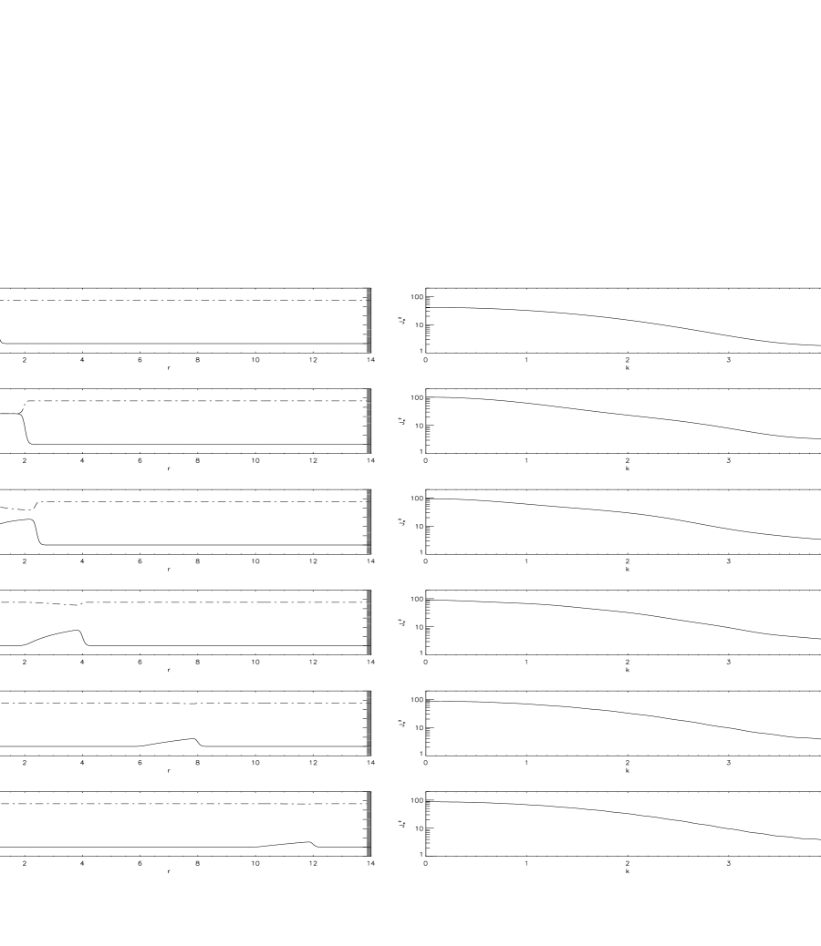
Figure 1: Evolution of the $\pi$ (continuous line) and $\sigma$ (broken line) fields according to the classical nonlinear sigma-model, starting from pure DCC $\pi=f_{\pi}$ inside the light-cone at $t=1fm$. The fields are shown in the snapshots on the left, whereas the snapshots on the right show the modulus squared of the pion source function (the $\tilde{J}$ of Eq. (20)). The horizontal scales for the left-side and right-side plots are in fermi and $($fermi$)^{-1}$ respectively.

4.4 Correlation between generic and DCC pion production

The question of correlations between generic and DCC pion production is very important for experimental DCC searches. It is quite reasonable that such correlations should exist. In our baked-alaska scenario, if the source strength on the light cone is large, i.e. lasts for a long time $T$, then the amount of DCC which is produced will, as we have seen, also be large. To be more quantitative is not easy. Here we attempt to make the connection by a simple argument based on energy densities. In the absence of the source, then there would be a surface-tension, i.e. an energy per unit area, associated with the boundary region between the sphere containing the DCC and the normal vacuum on the outside. It is contributed by the kinetic-energy term of the DCC hamiltonian, since gradients of the pion field exist in the interface region. It is reasonable to assume that when the energy per unit area of the generic partons or hadrons in the source region exceeds this surface energy, the inner DCC will be decoupled from the outer vacuum, and conversely when this energy is less than the DCC surface-tension, the source term will be inoperative. This will allow a connection between the amount of generic production and the amount of DCC produced.

In the spherically symmetric case, by assumption the DCC surface energy is contained in a shell of thickness $\Delta$, with $\Delta$ a typical hadronic scale, say $0.2fm<\Delta<0.6fm$. We can therefore write

$${E_{DCC}\over A}\sim{1\over 4\pi T^{2}}\int^{T}_{T-\Delta}dr\,4\pi r^{2}{1\over 2}f_{\pi}^{2}(\nabla\theta)^{2}\sim{f_{\pi}^{2}\over 2\Delta}~{},$$ (70)

where the last approximation on the right-hand side follows from approximating the profile at decoupling of the $\theta$-field near $r=T$ with a linear interpolation between $\theta(r=T-\Delta,t=T)=1$ and $\theta(r=T,t=T)=0$.

For the energy per unit area of the hot shell made of collision debris, one easily finds

$${E_{shell}\over A}={dE_{shell}\over dA}\sim\left[{<p_{T}>\,{dN\over d\Omega}d\Omega\over T^{2}d\Omega}\right]_{generic}=\left[{<p_{T}>\over T^{2}}{dN\over d\Omega}\right]_{generic}~{}.$$ (71)

If indeed at $t=T$ the DCC surface energy density equals the energy per unit area of the hot shell of collision debris, one finds from (70) and (71) that

$$\left[<p_{T}>{dN\over d\Omega}\right]_{generic}=T^{2}{f_{\pi}^{2}\over 2\Delta}~{}.$$ (72)

The aforementioned correlation between generic and DCC pion production is then seen upon combining (72) with (52) and (58). Specifically, one finds (in the chiral limit)

$$\left[p{dN\over d\Omega dp}\right]_{DCC}\sim{2\pi\over\Delta}\left[<p_{T}>{dN\over d\Omega}\right]_{generic}~{}.$$ (73)

We therefore see that it is possible for DCC production and generic production to be comparable in terms of the number density of produced particles.

5 Beyond the classical nonlinear sigma-model

Up to this point we have based our description of DCCs on linear, semiclassical, coherent-state solutions of a simple nonlinear sigma-model. However, there has been a considerable body of work on DCC production which goes substantially further. Not only are the nonlinear equations of the linear sigma-model (or even more complicated models [22]) considered, but also the effects of quantum fluctuations are taken into account within the mean-field [13, 23] (or large-$N$ [13, 14]) approximation. This level of calculation has become the de facto “state-of-the-art”. However, in most cases the space-time geometry is greatly simplified, or else the approach is aggressively numerical.

The closest calculation at this level to what we have presented here has been performed by Lampert, Dawson and Cooper (LDC) [18]. They consider a boost-invariant spherical expansion, such that the fields depend only upon the proper time which has elapsed since the expansion began. This is not very realistic, because the inclusive particle distribution which emerges must be the same in all reference frames, and therefore requires an infinite mean energy per particle, and an infinite formation-time for the final-state distribution.

While the LDC solutions are, as they stand, not very realistic, it is not too hard to adapt them to the baked-alaska scenario which we have described. We shall sketch in subsequent subsections how this works. The main point is that if we assume that the dynamics is as described in LDC for times $t$ less than $T$, after which time the sources on and near the light cone are turned off, then by causality the LDC solution will still be exact within the double-cone region, i.e. between the forward light-cone (vertex at $t=0$) and an inverted light cone with vertex at $t=2T$. If $T$ is large enough, one could hope that the fields inside the double-cone region and far from the light-cone be asymptotic, so that they could be matched onto the nonlinear sigma-model fields we use, and an estimate of the low-momentum portion of the particle spectrum could then be obtained using Eq. (20). The quality of this method can be tested by varying $T$ and determining which portion of the inclusive spectrum is insensitive to $T$.

For a more rigorous analysis of the spectrum, the source should be turned off at the decoupling time $T$, but the fields should be evolved according to the linear sigma-model up to times late enough for the evolution to be effectively free. At sufficiently late times one can then reliably extract the information on the inclusive spectrum using the procedure described in Sec. 4.

It is also instructive to consider the simplification achieved by neglecting the mean-field quantum corrections, in which case the LDC calculation is reduced to the solution of coupled ordinary differential equations describing the evolution of the classical fields in proper time. We have made such calculations for initial conditions chosen by LDC, and find remarkably close agreement of the time dependence of the pi and sigma fields with what is obtained from the full mean-field quantum calculation. This is encouragement that, when one goes on to consider the linear sigma-model in more difficult, less symmetric geometries, a classical calculation may well suffice to provide at least a semiquantitative picture of the dynamics which the mean-field calculation would provide. After all, only a semiquantitative description need be obtained from the linear sigma-model, because it is just a rough approximation to the complete low-energy effective chiral Lagrangian of real QCD.

In the following subsections we sketch more details of this line of argument. In subsection 5.1 we discuss the connection between the pion flux as calculated from the nonlinear sigma-model with what one would obtain from a classical solution of the linear sigma-model. In subsection 5.2 we describe in more detail the LDC analysis, especially in the classical approximation, and we numerically compare the mean-field and classical LDC-type solutions. In subsection 5.3 we match the classical versions of the LDC solutions at time $T$ onto the free asymptotic fields of the nonlinear sigma-model, thereby defining an effective source function $J$, from which the pion distributions are calculated. Finally, in subsection 5.4 we match the LDC solutions at time $T$ onto fields of the linear sigma-model, evolve according to the linear sigma-model up to some time $T^{\prime}$ say (late enough for the evolution to be effectively that of a free field) when the calculated effective source function will represent the actual pion flux.

5.1 Deriving the pion flux in more general frameworks

We start by applying our formalism to the derivation of the pion flux for the full linear sigma-model or related models, rather than for the nonlinear sigma-model considered in the previous sections. Provided one is dealing with a well-defined scattering problem, with the sources localized in space and time, the evolution of the $\pi$ and $\sigma$ degrees of freedom will eventually reach an asymptotic regime governed by free field behavior. An estimate of the associated inclusive pion spectrum can indeed be obtained by applying the formulas discussed in the previous sections.

While technically this procedure is rather straightforward, it is important to realize that the associated “sources” are somewhat different from the ones we have been discussing. In this more general case one is actually dealing with “effective sources”, useful as computational tools in the analysis of pion production, but not to be interpreted as physical external sources in the problem. From the point of view of the original model, say the linear sigma-model, these effective sources are given by the sum of a physical external source and a term from the self-interactions of the fields.

These ideas are of rather general applicability; for example, in the investigation of an interacting system described by the Lagrangian density

$${\cal L}={1\over 2}(\partial_{\mu}\Phi)(\partial^{\mu}\Phi)-{m^{2}\over 2}\Phi^{2}-V(\Phi)~{}$$ (74)

one is naturally led to the study of the evolution equation

$$(\Box+m^{2})\Phi=-V^{\prime}(\Phi)+J~{},$$ (75)

where $J$ is a physical “external” ($\Phi$-independent) source and $J_{\it eff}\equiv-V^{\prime}(\Phi)+J$ is an effective source.

The simulation reported in Fig. 2 corresponds to the linear sigma-model classical evolution from an initial configuration given by pure DCC, $\pi=f_{\pi}$, inside the light-cone and true vacuum outside (i.e. a snapshot of the solution (64) at some chosen time) and vanishing initial field velocities (except on the light cone). We simulate the classical field equations, as obtained from the Lagrangian density (21), for a spherically symmetric field configuration. Rather than simulating the $\Phi$ field directly, our program evolves $r\,\Phi(t,r)$ which simplifies the form of the d’Alambertian. The boundary conditions at the origin are set up to ensure that $\Phi(t,r)$ is an even function of $r$ at all times. The relevant classical field configuration is then evolved in time, using a simple staggered leapfrog algorithm (see for example [24]). The Fourier transforms involved in finding the source current $\tilde{J}(\vec{k})$ as defined in expression (20) are done using a straightforward (extended trapezoid) method. Fig. 2 shows a selection of output snapshots chosen to illustrate the main features of the evolution. The pictures on the left describe the evolution of the pion and sigma fields, while the pictures on the right describe the corresponding “evolution” of the Fourier-space effective source function. The emergence of a stationary Fourier-space effective source (which encodes the information on particle production) reflects the fact that at late times the evolution of the $\pi$ and $\sigma$ degrees of freedom reaches an asymptotic regime ruled by the nonlinear sigma-model. However, it should be noted that the low momentum part of the spectrum is only complete after a time scale between $4$ and $8$ fermi, and is significantly larger (a factor of $2$) than what was obtained for the nonlinear sigma-model for identical initial conditions.

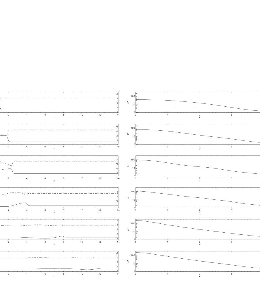
Figure 2: Evolution of the $\pi$ (continuous line) and $\sigma$ (broken line) fields, and the pion source function according to the linear sigma-model, starting from pure DCC $\pi=f_{\pi}$ inside the light-cone at $t=1fm$.

5.2 Classical version of LDC approach and reliability of coherent-state descriptions

Our description of DCCs uses the classical equations of motion to obtain an “out” field from a given “in” field. This “out” field is then mapped into a corresponding coherent state from which particle production (a quantum effect) can be derived. Some elegant recent studies [13, 14, 18] have been based on more general formalisms for the description of quantum effects and have taken into account (some of) the non-perturbative quantum effects contributing to the structure of the full propagator. One is then confronted with the solution of a genuinely non-classical evolution problem, in which “gap equations” describing the full propagators are combined with (modified) evolution equations for the fields. Seen as solutions of a variational problem, these equations result from finding an extremum of the (quantum) effective action for composites[25], just like the classical evolution equations are obtained from finding an extremum of the classical action for (local/non-composite) fields.

In Ref.[18], LDC investigated the chiral phase transition by modeling the relevant hadron dynamics with a linear sigma-model, and adopting evolution equations that take into account part of the non-perturbative quantum effects contributing to the structure of the full propagator via the familiar large-$N$ formalism. They concentrated on boost-invariant spherical expansions, such that the mean-field expectation values depend only upon the proper time $\tau\!=\!\sqrt{t^{2}-r^{2}}$. We refer the interested reader to Ref.[18] for the complete description of the LDC approach. For the purposes of the analysis presented in the remainder of this section, it is sufficient for us to consider explicitly the evolution equations corresponding to the classical version of the LDC equations, i.e. obtained from the LDC equations by dropping all contributions coming from the dressing of the propagator:

$$\left[{1\over\tau^{3}}{\partial\over\partial\tau}\left(\tau^{3}{\partial\over\partial\tau}\right)+\lambda(\sigma^{2}+{\bf\pi}^{2}-f_{\pi}^{2})\right]\sigma=f_{\pi}m_{\pi}^{2}$$ (76)

$$\left[{1\over\tau^{3}}{\partial\over\partial\tau}\left(\tau^{3}{\partial\over\partial\tau}\right)+\lambda(\sigma^{2}+{\bf\pi}^{2}-f_{\pi}^{2})\right]\pi=0~{}.$$ (77)

As a preliminary test of the reliability of our description of DCCs based on the classical evolution equations, we have compared the results for the mean-field evolution of the $\pi$ and $\sigma$ fields obtained in Ref.[18], to the corresponding results from the classical equations (76)-(77). In Fig. 3 the results of this comparative analysis are reported for the initial conditions singled out in Ref.[18] as the most “DCC-favoring” within the special family of initial conditions considered there; specifically, we integrate the fields from the initial conditions

$$\sigma=0~{}fm^{-1}~{}~{} \dot{\sigma}=-1~{}fm^{-2}$$

$$\pi=0.3~{}fm^{-1} \dot{\pi}=0~{}fm^{-2}$$ (78)

at $\tau=1~{}fm$. Since the focus of this exercise is only on the field evolution, rather than particle production, for simplicity we kept the exact (spherically-symmetric and boost-invariant) source structure adopted in Ref.[18]. Fig. 3 suggest that even at a quantitative level the description might be satisfactorily accurate. This is especially so because one is in any case using rough models of the relevant hadron dynamics (i.e. it appears to be likely that the inaccuracies introduced by using classical evolution equations might be less important than the ones resulting from modeling the relevant hadron dynamics with, say, the linear sigma-model).

Figure 3: Evolution of the pion and sigma fields as functions of proper time in the LDC setup. The continuous line corresponds to the purely classical analysis, whereas the dotted line corresponds to the quantum analysis reported in Ref. [18]. At proper time $\tau\!=1fm$ the fields and their derivatives are fixed to be $\pi=0.3fm^{-1}$, $\sigma\!=\!0fm^{-1}$, $\dot{\pi}\!=\!0fm^{-2}$, $\dot{\sigma}\!=\!-1fm^{-2}$.

5.3 Low-momentum portion of the inclusive spectrum in the LDC approach

As explained at the beginning of this section, the spherical expansion investigated in Ref.[18], which is fueled by everlasting sources, and involves fields depending upon only the proper time, is not very realistic. Still, as mentioned above one could attempt to extract the low-momentum portion of the inclusive pion spectrum associated with a baked-alaska-type modification of the LDC approach, by mapping the LDC solutions at time $T$ onto free asymptotic fields of the nonlinear sigma-model, thereby defining an effective source function $J$, from which the pion distributions are calculated. Ideally, one might find that for large enough $T$ the fields inside the double cone region be almost everywhere asymptotic, and that only the high-momentum tail of the particle spectrum could not be captured by such an approach. In practice, however, we find that not even the portion of the inclusive pion spectrum with very low momentum is well determined at times as late as $50~{}fm$.

In Fig. 4 we report the results of one such analysis, in which we integrate the fields from the initial conditions (78) at $\tau=1~{}fm$, to some later time $T$ and use the boost symmetry to reconstruct the fields everywhere on the $t=T$ surface inside the light cone. $\tilde{J}(\vec{k})$ is then extracted from this field configuration using Eq. (20) as before. The $\sigma$ and $\pi$ field configurations and the effective source function described for various choices of the above-mentioned time $T$ in Fig. 4 clearly reflect the shortcomings of the approach discussed in this subsection.

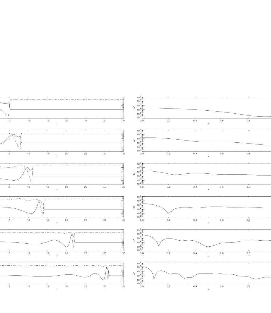
Figure 4: Evolution of the $\pi$ (continuous line) and $\sigma$ (broken line) fields, and the pion source function according to the classical linear sigma-model, in the presence of a boost-invariant and spherically invariant source considered in Ref. [18]. Again, the initial conditions are chosen according to the “DCC-favoring” scenario considered in Ref. [18].

5.4 LDC approach with truncated sources

The deficiencies of the method discussed in the previous section can be easily remedied. Evidently, after the external source is turned off at the decoupling time $T$, the fields should be evolved according to the linear sigma-model up to times late enough for the evolution to be effectively ruled by free field behavior. At such late times one can reliably extract the information on the inclusive spectrum using the procedure described in Sec. 4.

In Fig. 5 we report the results of such a simulation, again as snapshots describing the evolution of the fields and the effective source function corresponding to the initial configuration singled out as “DCC-favoring” in Ref.[18]. For illustrative purposes we chose in this simulation a large decoupling time ($5fm$). In this case the effective source does reach a stationary regime; however, by comparison with Fig. 2 we see that this asymptotic behavior only emerges at rather late times ($\sim 20-30~{}fm$). The comparison of Fig. 4 and 5 shows that the approach discussed in the preceding subsection, in which the LDC sources were never turned off, can largely overestimate (e.g. by more than a factor 10 if $T\leq 5fm$, as assumed in Fig. 5) even the low-momentum portion of the spectrum.

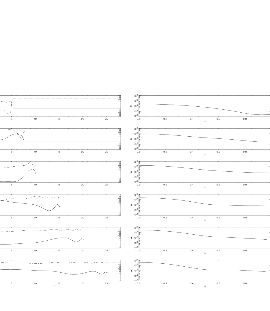
Figure 5: Evolution of the $\pi$ (continuous line) and $\sigma$ (broken line) fields, and the pion source function according to the linear sigma-model, in the presence of a truncated version (as described in the text) of the a boost-invariant and spherically invariant source considered in Ref. [18]. The source is switched off at $t\!=\ 5fm$.

6 Conclusions

In this paper we have investigated the various stages of the evolution of disoriented chiral condensates via the “baked-alaska” mechanism. Most of our analysis has been elaborated using classical equations of motion based on either the linear or nonlinear sigma model. The associated framework of coherent states was then used to make the connection with the distribution functions for the particle production. Important in this step is the identification of the source-function of the produced particles, namely the right-hand side of the usual wave equation (cf. Eq. (75)). The square of the on-shell fourier transform of this source function, as determined from the solutions of the equations, then provides directly the inclusive distribution of particles.

In general the source term consists of two parts. One is concentrated near the light cone, and is a genuine external source, not a function of the chiral fields, to be associated with the generic collision debris of partons, constituent quarks, etc. The other part consists of the nonlinear terms, built from the chiral fields themselves, which appear in the classical wave equation. We found evidence, within the nonlinear sigma-model approach, that the number of produced DCC pions is likely correlated with the number of generic hadrons produced, with this correlation local in (lego) phase-space. The number of DCC pions could be comparable with the number of generic hadrons according to this crude estimate, but the uncertainties are very large.

We also compared our very simple classical approach with a mean-field calculation which includes one class of quantum corrections, and at least in the case we studied, the quantum effects appear not to be of great importance. This is encouragement that, when attempts to go beyond the spherical symmetry assumed in this work, the simpler classical approach may suffice to reveal most of the important physics.

In all of the work in this paper (and in most of the literature), we have assumed spherical symmetry of the solutions. Regrettably, this geometry is too simple for many realistic applications. The intrinsic sources are reasonably uniform in lego variables, not spherical coordinates, and this geometry needs more detailed study. In addition, fluctuations about the mean behavior are very important. A piece of DCC with relatively large transverse velocity will look in the laboratory like a coreless minijet, with contents containing small relative momenta. So the source distributions most relevant to DCC searches in high energy hadron collisions should not only be described in lego variables, but also contain minijet clusterings.

However, in defense of what we do, each piece of DCC in momentum space is a cluster of pions of near identical momenta — a “snowball” — which has a local rest frame [2, 10]. In a snowball rest-frame, the calculations we make should be a reasonable description of the dynamics of that particular snowball. But one needs to know how the chiral orientations and probability of occurrence of snowballs which are neighboring in momentum-space are correlated. Very little work on this exists.

In addition, one should average over sources more broadly. This includes not only the properties of the intrinsic sources discussed above, but also the initial conditions imposed on the chiral fields at early proper time, i.e. at the onset of the chiral symmetry breaking. A good starting point will be to do this for the classical version of the interesting model of Lampert, Dawson, and Cooper [18], truncated at large times as described in this paper.

The final product of all this should be a generating functional for DCC particle production, which is an average over sources of a Gaussian generating functional characteristic of a coherent-state and classical solution produced by a specific source (see, for example, reference [20] for the formalism). However, even when this is attained, it still leaves open the more difficult problem of synthesizing such a generating functional with one for generic production, since there is not yet a consensus on what represents a good choice for the latter.

The emphasis we make in this paper on DCC sources makes the formalism look more and more similar to what is used to describe Bose-Einstein correlations [20]. There is certainly a close relationship [26]. What we believe special about the baked-alaska scenario, even accepting only the broad outlines, is that there is assumed to be nontrivial dynamics occurring deep within the future light cone. Irrespective of details of our modeling, the presence of such dynamics would be a new element in the description of hadron-hadron collisions at high energies.

References

- [1] A. A. Anselm, Phys. Lett. B217 (1989) 169; A. A. Anselm and M. C. Ryskin, Phys. Lett. B266 (1991) 482.
- [2] J. D. Bjorken, Int. J. Mod. Phys. A7 (1992) 4189; Acta Phys. Pol. B23 (1992) 561.
- [3] K. Rajagopal and F. Wilczek, Nucl. Phys. B379 (1993) 395; B404 (1993) 577.
- [4] J.-P. Blaizot and A. Krzywicki, Phys. Rev. D50 (1994) 442.
- [5] J. D. Bjorken, K. L. Kowalski and C. C. Taylor, SLAC-PUB-6109, in the proceedings of Les Rencontres de Physique de la Vallée D’Aoste, La Thuile (1993); hep-ph/9309235, in the proceedings of Workshop on Physics at Current Accelerators and the Supercollider, Argonne (1993).
- [6] S. Gavin, A. Gocksch and R. D. Pisarski, Phys. Rev. Lett. 72 (1994) 2143;
- [7] M. Asakawa, Z. Huang and X.-N. Wang, Phys. Rev. Lett. 74 (1995) 3126; Z. Huang and X.-N. Wang, Phys. Rev. D49, 4335, (1994); Z. Huang, I. Sarcevic, R. Thews and X.-N. Wang, Phys. Rev. D54 (1996) 750.
- [8] I.V. Andreev, Pisma v JETP 33 (1981) 384; S. Pratt, Phys. Lett. B301 (1993) 159.
- [9] I.I. Kogan, JETP Lett. 59 (1994) 307; R.D. Amado and I.I. Kogan, Phys. Rev. D51 (1995) 190.
- [10] J.D. Bjorken, SLAC-PUB-6488, in the proceedings of Workshop on Continuous Advances in QCD, Minneapolis (1994).
- [11] G. Amelino-Camelia, J.D. Bjorken, S.E. Larsson, hep-ph/9610202, in the proceedings of 10th International Conference on Problems of Quantum Field Theory, Alushta (1996).
- [12] A.A. Anselm, M.C. Ryskin and A.G. Shuvaev, Z. Phys. A354 (1996) 333.
- [13] D. Boyanovsky, H. J. de Vega and R. Holman, Phys. Rev. D51 (1995) 734.
- [14] F. Cooper, Y. Kluger, E. Mottola and J.P. Paz, Phys. Rev. D51 (1995) 2377; F. Cooper, Y. Kluger and E. Mottola, hep-ph/9604284.
- [15] Fermilab test/experiment T-864 (J. Bjorken and C. Taylor, spokesmen), “MiniMax”; for further information consult http://fnmine.fnal.gov.
- [16] K. L. Kowalski and C. C. Taylor, Disoriented Chiral Condensate: A White Paper for the Full Acceptance Detector, CWRUTH-92-6 (1992) hep-ph/9211282.
- [17] V. Karmanov and A. Kudrjavtsev, The Centauro Events as a Result of Induced Pion Emission, ITEP-88 (1983).
- [18] M.A. Lampert, J.F. Dawson, F. Cooper, Phys. Rev. D54 (1996) 2213.
- [19] H. Georgi and A. Manohar, Nucl. Phys. B234 (1984) 189.
- [20] I.V. Andreev, M. Plümer, and R.M. Weiner, Int. J. Mod. Phys. A8 (1993) 4577.
- [21] M. Birse, private communication
- [22] L.P. Csernai and I.N. Mishustin, Phys. Rev. Lett. 74 (1995) 5005; A. Abada and M.C. Birse, Phys. Rev. D55 (1997) 6887.
- [23] G. Amelino-Camelia, hep-ph/9702403, Phys. Lett. B (in press).
- [24] W.H. Press et al., Numerical Recipes in C, 2nd ed. Cambridge University Press (1992).
- [25] J.M. Cornwall, R. Jackiw, and E. Tomboulis, Phys. Rev. D10 (1974) 2428; G. Amelino-Camelia and S.-Y. Pi, Phys. Rev. D47 (1993) 2356; R. Jackiw and G. Amelino-Camelia, hep-ph/9311324, in Proceedings of the Third Workshop on Thermal Field Theories and Their Applications, Banff (1993).
- [26] I.V. Andreev, hep-ph/9612476.