Measuring Polarized Gluon and Quark Distributions with Meson Photoproduction

Abstract

We calculate polarization asymmetries in photoproduction of high transverse momentum mesons, focusing on charged pions, considering the direct, fragmentation, and resolved photon processes. The results at very high meson momentum measure the polarized quark distributions and are sensitive to differences among the existing models. The results at moderate meson momentum are sensitive to the polarized gluon distribution and can provide a good way to measure it. Suitable data may come as a by-product of deep inelastic experiments to measure $g_{1}$ or from dedicated experiments.

I Motivation

In this article, we will discuss photoproduction of high transverse momentum pions from polarized initial states. There are three motivations for doing so. One is the opportunity to learn the polarization distribution of quarks and gluons in nucleons. We will show that pion photoproduction with polarized initial states has, over a wide kinematic region of moderate transverse momentum pions, a large sensitivity to the polarized gluon distribution functions of the target. Within this wide kinematic region there are broad circumstances where the known polarized quark distributions all give similar pion photoproduction contributions, so that differences among the results are due mainly to the polarized gluon distributions. Hence data where rather ordinary mesons are produced can select among the various models for this quantity.

Another motivation, which we have written something about earlier [1], comes from the kinematic region of very high transverse momentum pions where the gluon contributions are small but the differences among the various models for the polarized quark distributions are significant. Hence examining different kinematic regions of pion photoproduction yields information about both polarized quark and polarized gluon distributions.

A third motivation, also dependent upon the highest transverse momentum pions, is the possibility of learning something about the pion distribution amplitude. In this region, ratios of cross sections determine the target’s quark distributions, but the magnitude of the cross section depends upon the same integral involving the pion distribution amplitude that enters the pion electromagnetic form factor of the $\pi^{0}\gamma\gamma^{*}$ vertex. Hence if one looks at the unpolarized case, where the target distributions are fairly well known, one has another measure of this integral. (Pion photoproduction in the unpolarized case has been well and successfully studied theoretically and experimentally [2], but not at the highest transverse momenta where the pions will be dominantly produced in a short distance process rather than via fragmentation [1, 3, 4].)

Presently, information on polarized quark distributions comes from deep inelastic electron or muon scattering with polarized beams and targets [5]. Single arm measurements of $g_{1}$ give information about a charge-squared weighted combination of polarized quark distributions. Obtaining polarized distributions of individual flavors is not possible from this data alone, but requires extra theoretical input in the analysis. Coincidence measurements of $\vec{\ell}\ \vec{p}(\vec{d})\rightarrow\ell\,\pi^{\pm}X$ give more information and have been reported [6]. This data, for a proton or deuteron target, gives different linear combinations of up and down quark polarized distributions, allowing a flavor decomposition without further theoretical input [7].

Polarized gluon distributions are not well determined at present. Something is learned from [8, 9, 10, 11] the measurements of $g_{1}$, but gluons contribute to $g_{1}$ only in higher order or through their effects upon the evolution of the polarized quark distributions. The analyses of $g_{1}$ can be abetted by perturbative QCD considerations at high $x$ [8]. Overall, however, the present constraints upon the polarized gluon distributions are not great and there is a large variance among $\Delta g(x,\mu^{2})$ models, as may be seen in Fig. 1.

The process we discuss, $\vec{\gamma}\,\vec{p}\rightarrow\pi\,X$ (where the photon is real and targets other than protons are possible), gives a complementary way to find the polarized quark distributions and is sensitive to the gluon distributions in leading order. The perturbative QCD that we use in the analysis is justified on the basis of high meson transverse momentum, rather than by high virtuality of an exchanged photon, and the experiment is a single arm experiment rather than a coincidence one. Good data can in fact come as a by-product of a $g_{1}$ experiment since the detectors that measure the final electron or muon can also pick up charged hadrons; recall that if the final lepton is not measured, the form of the cross section ensures that the virtuality of the exchanged photon will in general be rather low.

FIG. 1.: A number of polarized gluon distributions, all normalized to the unpolarized BBS gluon distribution. The sources of these distributions are given later in the text.

There are several processes that produce pions. At the highest transverse momenta, mesons are produced by short range processes illustrated in Fig. 3. We call these direct processes because the photon interacts directly with the target partons and also the pion is produced immediately. (The word “direct” was used with a similar meaning in a $\pi N\rightarrow\gamma^{*}X$ context by Brodsky and Berger long ago [12].) Direct processes are amenable to perturbative QCD calculation [3, 4] and produce mesons that are kinematically isolated in the direction they emerge. These processes possess several nice features. One is that if the pion three-momentum is measured, no integrals are needed to calculate the differential cross section. In particular, the momentum fraction $x$ of the struck quark is fixed by measurable quantities. Formulas for $x$ were given in [1] and will be repeated below, this time including mass corrections. The situation is reminiscent of deep inelastic lepton scattering, where experimentally measurable quantities, $Q^{2}$ and $\nu$, determine the quark momentum fraction by $x=Q^{2}/2m_{N}\nu$. Another nice feature is that the asymmetry for the meson production subprocess is easy to calculate and is large. Finally, mesons of a given flavor come mainly from quarks of a given flavor. Hence in the region where the direct process dominates, we can choose which flavor quark we study the polarization distribution of. Note that the high transverse momentum region involves only the high $x$ quarks and that the various models for the quark distributions separate from each other at high $x$.

At moderate pion transverse momentum, the main process is one we call the fragmentation process. The photon does interact directly with the partons of the target, but the meson is produced by fragmentation of one of the final state quarks or gluons. This time, an integration is needed to calculate the cross section, but any given model makes a definite prediction that can be compared to data. Unlike the case for $g_{1}$, interactions involving the gluons in the target contribute to the cross section in lowest order. One of the important subprocesses is photon-gluon fusion, $\gamma+g\rightarrow q+\bar{q}$. The polarization asymmetry of this process is very large. Indeed, neglecting masses, it is $-100$%: the process only goes if the photon and gluon have opposite helicity. Hence this process is even more significant for the polarization asymmetry than it is overall. There are situations where the results excluding the gluon polarization are close to the same for all the modern parton distribution function models or parameterizations. Then the differences among the results from different models are due to the polarized gluon distributions, and the differences over the spectrum of available models are large. Hence, the data will adjudicate among the different suggest polarized gluons distributions.

There is also the resolved photon process, where the photon turns into hadronic material before interacting with the target. We will discuss it in some detail below. However, for the kinematic situations we highlight, the resolved photon contributions are below both the fragmentation and direct contributions.

Calculational details are outlined in the following section. Some results and tests of the calculations are outlined in the next following section. Then, in section IV, we show results involving polarized initial states, in particular showing how sensitive the results are the the different models for the polarized parton distributions and how well they could be extracted from the data. Some conclusions will be given in section V.

II Calculations

There are three categories of processes that contribute to pion photoproduction and we call them fragmentation processes, direct processes, and resolved photon processes.

Fragmentation processes have quarks and gluons produced in short range reactions followed by fragmentation at long distances of either a quark or a gluon to produce the observed pion. The short distance part of the process is perturbatively calculated and the long distance part is parameterized as a fragmentation function for partons into pions. Direct processes, in our nomenclature, occur when the pion is produced in a short range reaction via a radiated gluon giving a quark-antiquark pair, one of which joins the initial quark to produce the pion. This process is perturbatively calculable, given the distribution of initial quarks, and produces isolated pions rather than pions as part of a jet. The direct process can dominate the fragmentation process for very high transverse momentum pions. Resolved photon processes are photons fluctuating into hadrons, most simply a quark-antiquark pair, which then interact with the partons of the target. The resolved photon processes can be important for high initial energy, especially for pions produced backward in the center of mass.

Fragmentation processes, of which one example is shown in Fig. 2, are important over a wide range of kinematics for the present paper, and we start by recording the relevant formulas [13]. In general, if the photon interacts directly with a constituent of target $N$ but the pion is produced as part of a jet,

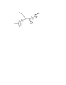
FIG. 2.: One diagram for photoproducing $\pi$ mesons via fragmentation.

$$\sigma=\sum_{a,c,d}\int G_{a/N}(x){d\hat{\sigma}\over d\hat{t}}(\gamma+a\rightarrow c+d)D_{\pi/c}(z)\,dx\,d\hat{t}\,dz.$$ (1)

Here, $x$ is the (light-cone) momentum fraction of the target carried by the struck parton $a$, $z$ is the fraction of the parton $c$’s momentum that goes into the pion, and $\hat{s}$, $\hat{t}$, and $\hat{u}$ are the Mandelstam variables for the subprocess $\gamma+a\rightarrow c+d$. The scale dependence of the parton distribution functions $G$ and the fragmentation functions $D$ will often be tacit, as it is above. As a differential cross section for the pion, one gets

$$E_{\pi}{d\sigma\over d^{3}k} = {s-m_{N}^{2}\over-\pi t}\sum_{a,c,d}\int_{z_{min}}^{1}{dz\over z}x^{2}\times$$ (3)

$$G_{a/N}(x){d\hat{\sigma}\over d\hat{t}}(\gamma+a\rightarrow c+d)D_{\pi/c}(z),$$

The Mandelstam variables for the overall process $s$, $t$, and $u$ are defined for the inclusive process by

$$s=(p+q)^{2}$$ (4)

$$t=(q-k)^{2}$$ (5)

$$u=(p-k)^{2}$$ (6)

where $q$, $p$, and $k$ are the momenta of the incoming photon, the target, and the outgoing pion, respectively. The lower integration limit is

$$z_{min}=-{t+u-m_{N}^{2}\over s-m_{N}^{2}},$$ (7)

and

$$x={-t\over z(s-m_{N}^{2})+(u-m_{N}^{2})}.$$ (8)

When the target and projectile are polarized, we define

$$\Delta\sigma={1\over 2}\left(\sigma_{R+}-\sigma_{R-}\right),$$ (9)

where $R$ and $L$ represent photon helicities and $\pm$ represent target helicities, and similarly for $\hat{\sigma}$. Also, the polarized parton distributions are defined by

$$\Delta G_{a/N}(x)=\Delta G_{a/N}(x,\mu^{2})=G_{a+/N+}(x)-G_{a-/N+}(x).$$ (10)

For quarks and gluons and proton targets we will often use the notation $q(x)\equiv G_{q/p}(x)$ and $g(x)\equiv G_{g/p}(x)$ and their polarized equivalents. The cross section is now given by

$$E_{\pi}{d\Delta\sigma\over d^{3}k} = {s-m_{N}^{2}\over-\pi t}\sum_{a,c,d}\int_{z_{min}}^{1}{dz\over z}x^{2}\times$$ (12)

$$\Delta G_{a/A}(x){d\Delta\hat{\sigma}\over d\hat{t}}(\gamma+a\rightarrow c+d)D_{\pi/c}(z).$$

The relevant subprocess cross sections are

$${d\hat{\sigma}\over d\hat{t}}(\gamma+q\rightarrow g+q) = {8\pi e_{q}^{2}\alpha\alpha_{s}\over 3\hat{s}^{2}}\left({-\hat{s}\over\hat{u}}+{\hat{u}\over-\hat{s}}\right),$$ (13)

$${d\hat{\sigma}\over d\hat{t}}(\gamma+g\rightarrow q+\bar{q}) = {\pi e_{q}^{2}\alpha\alpha_{s}\over\hat{s}^{2}}\left({\hat{u}\over\hat{t}}+{\hat{t}\over\hat{u}}\right),$$ (14)

$${d\Delta\hat{\sigma}\over d\hat{t}}(\gamma+q\rightarrow g+q) = {8\pi e_{q}^{2}\alpha\alpha_{s}\over 3\hat{s}^{2}}\left({\hat{s}\over-\hat{u}}-{\hat{u}\over-\hat{s}}\right),$$ (15)

$${d\Delta\hat{\sigma}\over d\hat{t}}(\gamma+g\rightarrow q+\bar{q}) = -{\pi e_{q}^{2}\alpha\alpha_{s}\over\hat{s}^{2}}\left({\hat{u}\over\hat{t}}+{\hat{t}\over\hat{u}}\right).$$ (16)

The cross section for $\gamma+q\rightarrow g+q$ is written for $\hat{t}$ being the momentum transfer between the photon and the gluon. The asymmetry for the quark target is positive and the asymmetry for the gluon target is $-100$%.

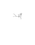
FIG. 3.: One of four lowest order perturbative diagrams for direct photoproduction of mesons from a quark. The four diagrams correspond to the four places a photon may be attached to a quark line.

For the direct process, the subprocess is shown in Fig. 3. When the incoming photon is circularly polarized and target quark is longitudinally polarized, one gets to lowest order

$${d\hat{\sigma}(\gamma q\rightarrow\pi q^{\prime})\over dt} = {128g_{F}^{2}\pi^{2}\alpha\alpha_{s}^{2}\over 27(-t)\hat{s}^{2}}I_{\pi}^{2}\left({e_{q}\over\hat{s}}+{e_{q^{\prime}}\over\hat{u}}\right)^{2}$$ (17)

$$\times \left[\hat{s}^{2}+\hat{u}^{2}+\lambda h\left(\hat{s}^{2}-\hat{u}^{2}\right)\right],$$ (18)

where $\lambda$ is the helicity of the photon, $h$ is twice the helicity of the target quark, and $g_{F}$ is a flavor factor from the overlap of the $q\bar{q}^{\prime}$ with the flavor wave function of the meson. It is unity for most mesons if the quark flavors are otherwise suitable; for example

$$g_{F}=\left\{\begin{array}[]{cc}1/\sqrt{2}&{\rm for\ }\pi^{0}\\ 1&{\rm for\ }\pi^{+}\end{array}\right..$$ (19)

The integral $I_{\pi}$ is given in terms of the distribution amplitude of the meson

$$I_{\pi}=\int{d\xi_{1}\over\xi_{1}}\phi_{\pi}(\xi,\mu^{2}).$$ (20)

It is the same integral which appears in the perturbative calculation of the $\pi^{\pm}$ electromagnetic form factor or of the $\pi^{0}\gamma\gamma$ form factor. For the asymptotic distribution amplitude, $\phi_{\pi}(\xi)=6\xi_{1}\xi_{2}\cdot f_{\pi}/2\sqrt{3}$, one gets $I_{\pi}=\sqrt{3}f_{\pi}/2$, where $f_{\pi}\approx 93MeV$. Finally, in this case

$$\hat{s}=(p_{1}+q)^{2},$$ (21)

$$\hat{u}=(p_{1}-k)^{2},$$ (22)

and $\hat{t}$ is the same as $t$.

The direct process is higher twist, nominally suppressed by a factor of scale $f_{\pi}^{2}/s$. However, for very high transverse momentum pions it is the dominant production process. When it is the dominant process, one can take advantage of the nice feature that the momentum fraction $x$ of the struck quark is completely determined by experimentally measurable quantities. With $p_{1}\simeq xp$ and estimating mass corrections with a proportional mass approximation, one has

$$\hat{s}+\hat{t}+\hat{u}=2x^{2}m_{N}^{2}.$$ (23)

Further,

$$\hat{s}=xs-x(1-x)m_{N}^{2},\quad\hat{t}=t,\quad\hat{u}=xu-x(1-x)m_{N}^{2}.$$ (24)

Hence,

$$x={-t\over s+u-2m_{N}^{2}}.$$ (25)

Thus to the overall process, the direct subprocess makes a contribution that requires no integration to evaluate. For the polarized case

$$E_{\pi}{d\Delta\sigma\over d^{3}k}={(s-m_{N}^{2})x^{2}\over-\pi t}{d\sigma(\gamma p\rightarrow\pi+X)\over dx\,dt}$$ (26)

$$\ ={(s-m_{N}^{2})x^{2}\over-\pi t}\sum_{q}\Delta G_{q/p}(x,\mu^{2}){d\Delta\hat{\sigma}(\gamma q\rightarrow\pi q^{\prime})\over dt},$$ (27)

where the helicity summations are tacit. The unpolarized case is the same with the $\Delta$’s.

We now come to the resolved photon contributions. One such contribution is illustrated in Fig. 4, where the photon turns into hadrons such as a quark-antiquark pair before interacting with the target.

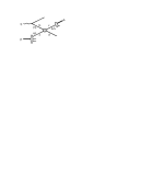
FIG. 4.: A resolved photon process.

The cross section is

$$E_{\pi}{d\Delta\sigma\over d^{3}k} = \sum_{abcd}\int_{y_{min}}^{1}dy\int_{z_{min}}^{1}dz\,{x^{2}(s-m_{N}^{2})\over-\pi zt}$$ (28)

$$\times \Delta G_{b/\gamma}(y)\,\Delta G_{a/N}(x){d\Delta\sigma\over d\hat{t}}D_{\pi/c}(z),$$ (29)

where again the scale dependence is tacit and the unpolarized case is got by removing the $\Delta$’s. Also,

$$x = {-yt\over yz(s-m_{N}^{2})+(u-m_{N}^{2})},$$ (30)

$$y_{min} = {-(u-m_{N}^{2})\over(s-m_{N}^{2})+t},$$ (31)

$$z_{min} = {-(u-m_{N}^{2})-yt\over y(s-m_{N}^{2})}.$$ (32)

For estimating the size of the resolved photon contributions, we began with the lowest order non-trivial result for the photon splitting function [13, 14],

$$G_{b/\gamma}(y)=3e_{b}^{2}{\alpha\over 2\pi}\left[y^{2}+(1-y)^{2}\right]\ln\left(Q^{2}\over Q_{0}^{2}\right)$$ (33)

and

$$\Delta G_{b/\gamma}(y)=3e_{b}^{2}{\alpha\over 2\pi}\left[y^{2}-(1-y)^{2}\right]\ln\left(Q^{2}\over Q_{0}^{2}\right),$$ (34)

with $Q_{0}=0.3$ GeV. In addition, we considered the more complete parametrizations [15] that use vector meson dominance to initialize the non-perturbative parton densities.

The subprocess cross sections, both polarized and unpolarized are available in [16]. For a quark or antiquark scattering off a gluon in the target,

$${d(\Delta)\sigma\over d\hat{t}}(qg\rightarrow qg)={\pi\alpha_{s}^{2}\over\hat{s}^{2}}\left(\hat{s}^{2}\pm\hat{u}^{2}\right)\left({1\over\hat{t}^{2}}-{4\over 9\hat{s}\hat{u}}\right),$$ (35)

where the upper and lower signs correspond to the unpolarized and polarized cases, respectively, and $\hat{t}$ is the momentum transfer from incoming to outgoing quark. For quark-quark (or antiquark-antiquark) scattering,

$${d(\Delta)\sigma\over d\hat{t}}(q_{\alpha}q_{\beta}\rightarrow q_{\alpha}q_{\beta}) = {\pi\alpha_{s}^{2}\over\hat{s}^{2}}{4\over 9}\biggl{\{}{\hat{s}^{2}\pm\hat{u}^{2}\over\hat{t}^{2}}$$ (36)

$$+ \delta_{\alpha\beta}\left[{\hat{s}^{2}\pm\hat{t}^{2}\over\hat{u}^{2}}-{2\hat{s}^{2}\over 3\hat{t}\hat{u}}\right]\biggr{\}},$$ (37)

where the coding of the $\pm$ is the same as above, the subscripts on $\delta_{\alpha\beta}$ refer to flavors of incoming quarks and $\hat{t}$ is the momentum transfer between incoming and outgoing quarks of the same flavor. (Note, of course, the $\hat{t}\leftrightarrow\hat{u}$ symmetry for the all same flavor case.) The last case is scattering of quark by antiquark,

$${d(\Delta)\sigma\over d\hat{t}}(q_{\alpha}\bar{q}_{\beta} \rightarrow q_{\delta}\bar{q}_{\gamma})={\pi\alpha_{s}^{2}\over\hat{s}^{2}}{4\over 9}\biggl{\{}\delta_{\alpha\delta}\delta_{\beta\gamma}{\hat{s}^{2}\pm\hat{u}^{2}\over\hat{t}^{2}}$$ (38)

$$\pm \delta_{\alpha\beta}\delta_{\gamma\delta}\left[{\hat{t}^{2}+\hat{u}^{2}\over\hat{s}^{2}}-\delta_{\alpha\delta}{2\hat{u}^{2}\over 3\hat{s}\hat{t}}\right]\biggr{\}},$$ (39)

where still again the upper and lower signs correlate with the unpolarized and polarized cases, $\hat{t}$ is the momentum transfer from incoming to outgoing quark, and $\alpha,\beta,\gamma$, and $\delta$ are flavor indices.

Good data can come from electroproduction experiments where only the outgoing pion is observed. Because of the $q^{-4}$ in the cross section, the photons are nearly all close to real, and the equivalent photon approximation gives the general connection between the electroproduction and photoproduction cross sections [17],

$$d\sigma(eN\rightarrow\pi X)=\int_{E_{min}}^{E_{e}}dE_{\gamma}\,N(E_{\gamma})d\sigma(\gamma N\rightarrow\pi X).$$ (40)

where $E_{\gamma}$ is the energy of the photon and

$$N(E_{\gamma}) ={\alpha\over\pi E_{\gamma}}\biggl{[}{E_{e}^{2}+{E^{\prime}_{e}}^{2}\over E_{e}^{2}}\left(\ln{E_{e}\over m_{e}}-{1\over 2}\right)+{E_{\gamma}^{2}\over 2E_{e}^{2}}\times$$ (41)

$$\times \left(\ln{2E^{\prime}_{e}\over E_{\gamma}}+1\right)+{(E_{e}+E^{\prime}_{e})^{2}\over 2E_{e}^{2}}\ln{2{E^{\prime}}_{e}\over E_{e}+E^{\prime}_{e}}\biggr{]},$$ (42)

where $E^{\prime}_{e}=E_{e}-E_{\gamma}$. The lower limit on the photon energy integral is

$$E_{min}={k\over 1-2(k/m_{N})\sin^{2}(\theta_{lab}/2)}.$$ (43)

When the electron is polarized, the polarization transfers nicely to the photon provided the photon takes most of the electron’s energy. Polarization details can be found in [18]; most usefully, if $P_{\gamma}$ and $P_{e}$ are the circular and longitudinal polarizations of the photon and electron, respectively, then

$${P_{\gamma}\over P_{e}}={y^{\prime}(4-y^{\prime})\over 4-4y^{\prime}+3y^{\prime 2}}.$$ (44)

where $y^{\prime}=E_{\gamma}/E_{e}$.

We close this section with a few comments on our procedures.

We used $\alpha_{s}(\mu^{2})$ with the renormalization scale set to the pion transverse momentum. Not all the pieces needed for are calculation are known beyond leading order and we have worked to lowest order throughout. We took $\Lambda_{QCD}=175$ MeV for four flavors. (This corresponds, to about $\pm\,6$% in $\alpha_{s}$ for $\mu=1-5$ GeV, to a four flavor $\Lambda_{QCD}$ of 295 MeV in the next to leading order formula, which matches to a five flavor $\Lambda_{QCD}$ of 209 MeV, which is the central value quoted by the Particle Data Group [19]. Uncertainties are roughly $\pm 40$ MeV on the 209 and 175 MeV numbers, and $\pm 50$ MeV on the 295 MeV.)

The fragmentation functions we use may be found in the Appendix of [3]. Briefly, the fragmentation of quarks into pions contains a part $D_{p}$ if the primary quark is a valence quark in the pion, and also a secondary part $D_{s}$ for any quark-pion combination. Three examples are

$$D_{\pi^{+}/u} = D_{p}+D_{s},\quad D_{\pi^{0}/u}={1\over 2}D_{p}+D_{s},$$ (45)

$$D_{\pi^{-}/u} = D_{s}.$$ (46)

At the benchmark scale (which we took to be 29 GeV),

$$D_{p}={5\over 6}(1-z)^{2}\quad{\rm and}\quad D_{s}={5\over 6}{(1-z)^{4}\over z}.$$ (47)

These forms lead to good fits to the $e^{+}e^{-}\rightarrow\pi+X$ data, and so we stick with them. At the time of reference [3], the known fragmentation functions were more than a decade old and no longer fit up-to-date data. Since then a number of other modern fragmentation functions have appeared [20], which also match data. The benchmark gluon fragmentation function is

$$D_{\pi/g}={2\over 3}{(1-z)^{3}\over z}.$$ (48)

The mass corrections we estimated using a proportional mass approximation. We gave the parton that came from the target a mass $xm_{N}$, and gave the final parton that did not go into the pion the same mass. The parton that did go into the pion we treated as massless (like the pion), and did the same for the parton that came from the photon in the resolved photon process. A fully defensible treatment of mass corrections would require a solution to QCD. The proportional mass approximation just described has the virtues of being simple and of giving the same kinematic limits from thresholds and energy conservation for the subprocess as for the overall process. Hence, it is an improvement over putting in no mass corrections, though we may treat it largely as a way to receive a warning to be careful when the mass corrections are big. For the situations we study, the mass corrections are not large except when the cross sections are very small.

III Results without Polarization

Our present main interest is on results obtainable for polarized beams and targets. However, both for checking the model and for intrinsic interest we will present some results with no polarization involved. First in Fig. 5 we show the relative size of the fragmentation, direct, and resolved photon contributions for some kinematics of interest, namely 50 GeV electrons with the only observed final state particle being a $\pi^{+}$ emerging at 5.5^∘ in the lab. The resolved photon curve used the simple perturbative parton densities in the photon given by eqn. (33). The resolved contributions are still small for our kinematics if one of the more realistic distributions be used. As an example, Fig. 5 also shows the resolved photon contribution using SaS 2D from the last of ref. [15]. It increases the resolved photon result by about 80% for the smallest momentum shown and then gives a smaller result for momenta above 13 GeV. In the kinematics of Fig.5, average fractions of the photon momentum carried by its partons are $<y>$=0.69 for the lowest pion momentum in Fig.5, 0.8 for momentum 15 GeV and 0.9 for momentum 24 GeV. Because of these large values of $<y>$, we neglected a possible gluon fusion process ($gg\to q\bar{q}$).

Commentary on the quark and gluon distribution models we use is put in the next section, so that we can bundle the remarks on the polarzed and unpolarized distributions into one location.

FIG. 5.: Comparing fragmentation, direct, and resolved photon processes for $e+p\rightarrow\pi^{+}+X$ with $E_{e}=50$ GeV and $\theta_{lab}=5.5^{\circ}$. These all use the GRSV parton distributions. The relative size of the contributions should not depend much on which parton distributions we use. For the resolved photon contribution, the result of both the perturbative splitting function for the photon, eqn. (33), and the more sophisticated SaS 2D are shown. Both are small for these kinematics.

One sees that the cross section falls quickly with increasing pion momentum. The fragmentation process is the main one at lower pion momenta, and the direct process takes over above about 26 GeV for this particular angle and incoming energy.

In addition, one sees that the resolved photon process is not particularly important here. At higher energies it increases in relative importance [21] and at HERA energies ($\sqrt{s}\approx 300$ GeV), the resolved photon process dominates except for very forward angles. The reason for its fast increase involves the lower average $y$ possible at higher energies, as well as the reduced kinematic constraint upon a three step (three integrals in the calculation) process as the energy increases.

The $\pi^{+}/\pi^{-}$ ratio off proton and neutron targets is shown in Fig. 6, again for 50 GeV incoming electrons. Most of the models for the parton distributions lead to the similar results except at the highest $k$, which will be discussed below. Also included in the figure are two sets of predictions for the $\pi^{+}/\pi^{-}$ ratio of isoscalar or nearly isoscalar targets.

FIG. 6.: The $\pi^{+}/\pi^{-}$ ratio for $E_{e}=50$ GeV and $\theta_{lab}=5.5^{\circ}$ for the pions. The dashed curve is for GRV and the solid curve is for CTEQ. Both have $u(x)/d(x)\sim 1/(1-x)$ for large $x$. The four pairs of curves are for, top to bottom, protons, a target which is 5/9 protons and 4/9 neutrons, an isoscalar target, and neutrons.

We detail in Fig. 7 the $\pi^{+}/\pi^{-}$ ratio for 50 GeV incident electrons on a target that is $5/9$ protons and 4/9 neutrons. (These are relevant numbers for one actual ammonia target, where the nitrogen is ¹⁵N and the hydrogens have plain proton nuclei.)

The predictions for the $\pi^{+}/\pi^{-}$ ratio are different for purely direct and purely fragmentation processes. For an isoscalar target, the ratio is not sensitive to the quark distributions, and the observed behavior of the $\pi^{+}/\pi^{-}$ ratio could be a clear signal for the direct process taking over from fragmentation with increasing pion momentum. For a proton or neutron target, there is much sensitivity to the quark distributions. The size of $d(x)$ vs. $u(x)$ at high $x$ is one of the remaining open questions for unpolarized quark distributions, and if it can be established that the high $x$—high $k$ results are mainly direct (or mainly fragmentation, if that should happen against our expectations) then the observed $\pi^{+}/\pi^{-}$ ratio becomes a direct measure of $d(x)/u(x)$.

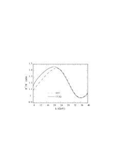
FIG. 7.: Detail of $\pi^{+}/\pi^{-}$ ratio for $E_{e}=50$ GeV and $\theta_{lab}=5.5^{\circ}$ for the pions, for a target which is $5/9$ protons and 4/9 neutrons.

To elaborate the preceeding remarks, consider what happens for $x$ approaching unity, where only valence quarks matter and $\pi^{+}$ comes from $u$ and $\pi^{-}$ comes from $d$. If fragmentation dominated, then

$$\left.{\pi^{+}\over\pi^{-}}\right|_{frag}=4\ {f_{p}u(x)+(1-f_{p})d(x)\over f_{p}d(x)+(1-f_{p})u(x)},$$ (49)

where the target is fraction $f_{p}$ proton. The “4,” of course, is $(e_{u}/e_{d})^{2}$. Also, for fragmentation, $u(x)$ and $d(x)$ must be understood as appearing inside some integrals, but only the ratio $d(x)/u(x)$ as $x\rightarrow 1$ will matter here.

For the direct case, the short distance nature of the reaction allows the photon to interact with the produced $q\bar{q}$ pair as well as with the target quark, so it makes less difference whether a $\pi^{+}$ or $\pi^{-}$ is produced. One has—see eqn. (18)—,

$$\left.{\pi^{+}\over\pi^{-}}\right|_{direct}=\left(s+2|u|\over 2s+|u|\right)^{2}{f_{p}u(x)+(1-f_{p})d(x)\over f_{p}d(x)+(1-f_{p})u(x)}.$$ (50)

The prefactor is less than one, but approaches one for small angles and maximum pion energy, when $|u|\rightarrow s$.

For isoscalar ($I_{3}=0$ suffices) or nearly isoscalar targets the $\pi^{+}/\pi^{-}$ ratio would approach 4 for maximum momentum in the fragmentation process, or approach 1 for the direct process, and be rising with momentum. One can qualitatively understand the curve shown for the near isoscalar case in Fig. 6: at low $k$, fragmentation dominates but the $\pi^{+}/\pi^{-}$ ratio is not large as there are important contributions from gluons and sea quarks in the target. As $k$ rises, the valence quark contributions become relatively more important and the ratio rises. Then the direct or short distance process takes over and the ratio falls, and finally rises a bit due to the prefactor in the last equation after the process is almost pure direct.

For a proton target, the $x\rightarrow 1$ limit of the ratio $d(x)/u(x)$ is important. Possibilities include,

$${d(x)\over u(x)}=\left\{\begin{array}[]{cl}0&\qquad{\rm many\ fits}\\ 1/5&\qquad{\rm pQCD}\\ 1/2&\qquad SU(6)\end{array}\right.$$ (54)

Both CTEQ [22] and GRV [23] have $u(x)$ and $d(x)$ falling with different powers of $(1-x)$, with $d(x)$ falling faster, and so are examples of the first category. The BBS [8] distributions, whose non-separation of $q$ and $\bar{q}$ is inconsequential at high $q$, do satisfy the pQCD constraint and so give a different $\pi^{+}/\pi^{-}$ ratio as the pion momentum reaches its maximum.

IV Results with Polarization

We have calculated the asymmetry $E$ (or $A_{LL}$) for $\pi^{\pm}$ photoproduction off both the proton and neutron. If $R$ and $L$ represent photon helicities and $\pm$ represent target helicities, then $E$ is defined by

$${E}\equiv{\sigma_{R+}-\sigma_{R-}\over\sigma_{R+}+\sigma_{R-}}.$$ (55)

The notation “$E$” comes from early pion photoproduction work (see for example [24]). We will now see how well we can achieve our goal of determining the polarized parton distributions from these experiments that measure $E$. We have direct sensitivity to the polarized gluon distribution $\Delta g(x,\mu^{2})$ since at moderate and lower momenta a reasonable fraction of the pions are produced by reactions off the gluons within the target. Other determinations of $\Delta g$ have depended upon higher order effects such as the evolution of the polarized quark distributions [11], which is driven in part by $\Delta g$.

FIG. 8.: The asymmetry $E$ for $\vec{\gamma}+\vec{n}\rightarrow\pi^{\pm}+X$, at $E_{e}=50$ GeV and $\theta_{lab}=5.5^{\circ}$. The upper six curves are for $\pi^{-}$ production and the lower six curves are for $\pi^{+}$ production. For each set of six, there are three curves with the full calculation, with the loose dotted curve using parton distributions from GRSV, the dashed curve using GS-A, and the tight dotted line using CTEQ/Soffer et al. and the BBS polarized gluon distribution. The other three curves have $\Delta g$ set to zero, with the solid line using GRSV, the dash-dot curve using GS, and the dash-triple dot curve using CTEQ/Soffer et al.

We will begin by presenting results for $\vec{\gamma}+\vec{n}\rightarrow\pi^{\pm}+X$ and for $\vec{\gamma}+\vec{p}\rightarrow\pi^{\pm}+X$ where the photon comes from radiation off an incoming electron beam of energy $E_{e}=50GeV$ and the pions are observed at lab angle $\theta_{lab}=5.5^{\circ}$. The outcome plotting asymmetry $E$ vs. the magnitude of the pion momentum is given in Figs. 8 and  9 using three differing sets of polarized parton models.

The polarized parton models are those of Gehrmann and Stirling (GS) [9], of Glück, Reya, Stratmann, and Vogelsang (GRSV) [10], and a suggestion of Soffer et al. [25]. Both the GS and GRSV polarized fits use the fits of Glück, Reya, and Vogt (GRV) [23] when they need unpolarized distributions, at least in leading order. For the first two, we have obtained the renormalization scale dependent results for the polarized parton distributions directly from the authors. The Soffer et al. suggestion relates the polarized and unpolarized distribution functions, specifically,

$$\Delta u_{V}(x) = u_{V}(x)-d_{V}(x),$$ (56)

$$\Delta d_{V}(x) = -{1\over 3}d_{V}(x),$$ (57)

and other polarized distributions are treated as small. When we use the Soffer et al. suggestion, we team it with the CTEQ [22] quark distributions and the polarized gluon distribution of Brodsky, Burkhart, and Schmidt (BBS) [8]. In addition this case requires a polarized distribution for the sea quarks, which we take as

$$\Delta s(x)=-0.667(1-x)^{7},$$ (58)

with the same sea distribution for up, down, and strange quarks. This gives $\langle\Delta s+\Delta\bar{s}\rangle=-1/6$. In all cases, we set the renormalization scale $\mu^{2}$ to $k_{T}^{2}$, where $k_{T}$ is the transverse momentum of the produced meson.

Although there are 12 different curves on Fig. 8, it is not so complicated. In all cases, $E$ is generally positive for the $\pi^{-}$ and negative for the $\pi^{+}$, so there are six curves above for the $\pi^{-}$ and six below for the $\pi^{+}$. Each of the three parton distribution models is represented twice, once with the full calculation and once with the polarized gluon distributions $\Delta g(x)$ (but not the total gluon distribution $g(x)$) set to zero.

Fig. 9, for the proton target, is similar except that $\pi^{+}$ is above and $\pi^{-}$ below.

One reaches the following conclusions from the graphs:

• At large pion momentum $k$ contributions from gluons in the target are not significant but the results for differing polarized quark distributions are quite different, allowing the data to discriminate among the various polarized quark distribution models. Note that for both the $\pi^{\pm}$ at high $k$, two of the models give quite similar results and one is different. However, for the $\pi^{-}$ it is CTEQ/Soffer et al. that is different, whereas for the $\pi^{+}$ it is GS that stands out.

• At low or moderate $k$ the results for the different model polarized quark distributions are—if evaluated with zero or the same $\Delta g$—rather similar. In the figures, we show the curves with $\Delta g=0$. The clearest case is $\pi^{-}$ production off a proton target.

• At low or moderate $k$, the differences among the models are mainly due to the differences in $\Delta g$ (even noting that the largest $\Delta g$ are not represented on these two figures), and thus the measurements can discriminate among the differing models for $\Delta g$.

FIG. 9.: The asymmetry $E$ for $\vec{\gamma}+\vec{p}\rightarrow\pi^{\pm}+X$, at $E_{e}=50$ GeV and $\theta_{lab}=5.5^{\circ}$. This time, the upper six curves are for $\pi^{+}$ production and the lower six curves are for $\pi^{-}$ production. As in Fig. 8, for each set of six, there are three curves with the full calculation, with the loose dotted curve using parton distributions from GRSV, the dashed curve using GS-A, and the tight dotted line using CTEQ/Soffer et al. and the BBS polarized gluon distribution. The other three curves have $\Delta g$ set to zero, with the solid curve using GRSV, the dash-dot curve using GS, and the dash-triple dot curve using CTEQ/Soffer et al.

We elaborate on the last point in Fig. 10, where we use only one quark distribution, but six different gluon distributions to show the differences in their effect upon this asymmetry. Two of the new polarized gluon distributions are from Ball, Forte, and Ridolfi (BFR) [11], and we use versions AR and OS. (Neither BBS nor BFR give quark distributions for each individual flavor quark and antiquark, so we can show results from their gluon distributions only in combination with other authors’s models for the quarks.) The other new polarized gluon distribution is GS version C. One can see that the available polarized gluon distributions, all inferred from $g_{1}$ data, sometimes abetted by pQCD considerations at high x [8], give distinct results in the present case.

Incidentally, the minimum $x$ that enters the calculation of the fragmentation process is the same as the unique $x$ that enters the direct process, Eqn. (25). Hence for the situation of Figs. 8 or 10, the minimum $x$ for pion momentum $k=8$ GeV is $x_{min}=0.05$ and for $k=20$ GeV, $x_{min}=0.16$. This gives some idea of the $x$ range that is probed by these experiments.

FIG. 10.: The asymmetry $E$ for $\vec{\gamma}+\vec{n}\rightarrow\pi^{\pm}+X$, at $E_{e}=50$ GeV and $\theta_{lab}=5.5^{\circ}$, with one model for the quark distributions and several models for the polarized gluon distribution. We choose to use the quark distributions of GS. The solid curve is the benchmark with $\Delta g$ set to zero. The short dashed curve uses the quark and unpolarized gluon distribution of GS but the polarized gluon distribution of GS model A. The long dashed curve uses GS model C. The dash dot curve uses GRSV. The dash triple dot curve similarly uses BBS, the tight dotted curve uses BFR model AR, and the loose dotted curve uses BFR model OS.

We continue showing results in Fig. 9 by giving the analog of Fig. 8 but for a proton target. The electron energy is still $E_{e}=50$ GeV and $\theta_{lab}=5.5^{\circ}$. The $\pi^{-}$ curves, which are the lower ones in this Figure, bunch very well at low $k$ for the three curves with $\Delta g$ set to zero, and the curves using the $\Delta g$ pertinent to each model are quite distinct. The $\pi^{+}$ curves are less distinct from each other, but it is still true that for the models chosen the curves with $\Delta g=0$ all lie, at low $k$, above the curves with gluon polarization included.

FIG. 11.: The asymmetry $E$ for $\vec{\gamma}+\vec{n}\rightarrow\pi^{\pm}+X$, at $E_{e}=27.5$ GeV and $\theta_{lab}=5.5^{\circ}$. The remainder of the caption is the same as for Fig. 8.

The next three figures show the analogs of the preceding three Figures but for an incoming electron energy of 27.5 GeV; the lab angle is still $\theta_{lab}=5.5^{\circ}$. Fig. 11 shows the asymmetry $E$ for $\pi^{\pm}$ production off a neutron target for the three models we have chosen, with and without $\Delta g$. Fig. 12 does the same for a proton target. The Figure with one quark distribution model but six polarized gluon distribution models is Fig 13. It is the analog of Fig. 10 , but for variation we have given this Figure with a proton instead of a neutron target.

V Discussion

We feel we have demonstrated that with polarized initial states, pion photoproduction at low (but still with $k_{T}$ above about 1 GeV) and moderate pion momenta can be a useful and successful way to learn about the polarized gluon distribution. In this region, the various models for the polarized quark distributions all give rather similar results when the effects of the polarized gluon distributions are removed. The effects of the polarized gluon distributions are distinct for the different models, and particularly for the BBS [8] and BFR [11] models are quite large. For the kinematics we have looked at, the resolved photon contributions are always small. In the low to moderate $k$ region, the fragmentation contribution is dominant.

At the highest allowed pion momentum the asymmetry does become sensitive to the differences among the various quark models, and so can empirically distinguish among them. What we call the direct process, i.e., pion production at short distance rather than via fragmentation, dominates in this region. In particular, the high $x$ quarks of the target give the dominant contributions and the models for the polarized quark distributions do not agree at high $x$.

FIG. 12.: The asymmetry $E$ for $\vec{\gamma}+\vec{p}\rightarrow\pi^{\pm}+X$, at $E_{e}=27.5$ GeV and $\theta_{lab}=5.5^{\circ}$. The remainder of the caption is the same as for Fig. 9.

Questions may be asked about the use of perturbative QCD, upon which our analyses depend. We are, of course, mainly considering ratios of cross sections so that many potential problems cancel out.

Also, studies of the polarized gluon distribution depend mainly upon the fragmentation process. This is a leading twist process, so using perturbation theory to calculate it should be accurate and has not generally been questioned.

Within the context of perturbation theory, one may ask how large the higher order in $\alpha_{s}$ corrections are. For the unpolarized case, the answer is that the next to leading corrections double the result [2]. We should state that we have simply doubled our lowest order calculations to obtain our results: remember we are taking ratios. We are not aware of NLO calculations of $\vec{\gamma}\vec{g}\rightarrow q\bar{q}$ or $\vec{\gamma}\vec{q}\rightarrow qg$. However, NLO calculations of $\vec{g}\vec{q}\rightarrow\gamma q$ and $\vec{q}{\vec{\bar{q}}}\rightarrow\gamma g$ and related $2\rightarrow 3$ processes have been done [26]. The $K$-factors [ratio of LO + NLO to LO cross sections] for the polarized cross section $\Delta\sigma$ always exceed unity, so that the effect of the NLO corrections upon the ratio $E$ for direct photon production is not great.

FIG. 13.: The asymmetry $E$ for $\vec{\gamma}+\vec{p}\rightarrow\pi^{\pm}+X$, at $E_{e}=27$ GeV and $\theta_{lab}=5.5^{\circ}$, with one model for the quark distributions and several models for the polarized gluon distribution. We use the quark distributions of GS. The upper set of curves is for the $\pi^{+}$ and the lower set is for the $\pi^{-}$; otherwise the caption is the same as Fig 10.

Much of our further discussion concerns the direct process, which is a higher twist contribution and using perturbative QCD has been questioned is some such cases. We can for completeness summarize some earlier arguments [1].

Our analysis requires that the “$X$” in $\gamma+p\rightarrow\pi+X$ is out of the resonance region. For the energies we have considered, this is easy to satisfy except at the highest $k$.

Another question regards further higher twist corrections, for example, corrections due to the quarks in the pion having finite momentum transverse to the pion’s overall momentum. This has been much studied in the context of the pion electromagnetic form factor [27]. In the present case, the virtual gluon in the direct process is much farther off shell [1, 3] than for the pion form factor at presently accessible kinematics. Hence higher twist effects will be less significant for measurable photoproduction of high transverse momentum mesons than for meson form factors at any currently measured momentum transfers. Similarly, we have not considered transverse momentum smearing of the incoming quarks. It has been considered in the context of pion production in $pp$ and $\bar{p}p$ collsions, and does have some effect there on the extraction of the polarized gluon distribution [28].

Perturbative corrections that are higher order in $\alpha_{s}$ have not been calculated. They may be calculated along the lines of [29] for the $\pi^{0}\gamma\gamma$ and of [30] for the $\pi^{\pm}$ electromagnetic form factors. For both of these, using the asymptotic distribution amplitude and a suitable choice of renormalization scale, the magnitude of the correction was about 20%, decreasing the $\pi^{0}\gamma\gamma$ and increasing the $\pi^{\pm}$ form factors.

Our calculations can also be applied to production of kaons and to neutral pions. For neutral pions, the fragmentation process cross section is the average of the $\pi^{+}$ and $\pi^{-}$ cross sections. However, the direct production of neutral pions is less than the direct production of either charged pion. Useful studies are also possible using single polarization asymmetries. We hope to return to these subjects in the near future.

We conclude with a summary.

• Of the three processes that contribute to high $k_{T}$ pion production, or to its single arm electron equivalent $e+N\rightarrow\pi+X$, the resolved photon process is unimportant for incoming energies of a few 10’s of GeV and small angles. The fragmentation process dominates at low or moderate momenta, the direct process dominates at high pion momenta.

• The $\pi^{+}/\pi^{-}$ ratio predictions are different for fragmentation and direct processes. For isoscalar or near isoscalar targets, with pions at high momenta, fragmentation would give about a 4:1 ratio [coming from $(e_{u}/e_{d})^{2}$] but the direct process gives about 1:1. Verification that short distance production takes over from fragmentation production lies in seeing a fall in the $\pi^{+}/\pi^{-}$ ratio (still for $I=0$ targets) as the takeover occurs.

• Where the direct process dominates, and without polarization, the rate is proportional to things that are known and the $I_{\pi}$, the same integral over the pion distribution amplitude that fixes $\gamma^{*}+\gamma\rightarrow\pi^{0}$ and $\gamma^{*}+\pi^{\pm}\rightarrow\pi^{\pm}$. Currently data for the last two processes taken at face value gives discordant values of $I_{\pi}$.

• With initial state polarization, one can form the double helicity asymmetry $A_{LL}$ or $E$. Where the direct process dominates, at high pion momentum, the asymmetry is proportional to the polarized quark distributions $\Delta u$ for the $\pi^{+}$ and $\Delta d$ for the $\pi^{-}$, times things that are known or easily calculable. Hence, one can measure the $\Delta q_{i}$ individually.

• When the fragmentation process dominates, experiments with initial state polarization are sensitive to $\Delta g$. The polarization asymmetry is 100% in magnitude for the production off a gluon target, and the current spectrum of models for $\Delta g$ leads to a wide diversity of $A_{LL}$ or $E$ predictions for pion photoproduction in the fragmentation region.

REFERENCES

- [1] A. Afanasev, C. Carlson, and C. Wahlquist, Phys. Lett. B 398, 393 (1997).
- [2] P. Aurenche et al., Phys. Lett. 135B, 164 (1984); E. Auge et al., Phys. Lett. 168B, 163 (1986).
- [3] C. E. Carlson and A. B. Wakely, Phys. Rev. D 48, 2000 (1993).
- [4] Similar processes in the context of annihilation were discussed by V. N. Baier and A. G. Grozin, Phys. Lett. 96B, 181 (1980) and by Th. Hyer, Phys. Rev. D 48, 147 (1993), ibid., 50, 4382 (1994).
- [5] D. Adams et al., Phys. Lett. B 329, 399 (1994); Phys. Lett. B 336, 125 (1994); Phys. Lett. B 357, 248 (1994); P. L. Anthony et al., Phys. Rev. Lett. 71, 959 (1993); K. Abe et al., Phys. Rev. Lett. 74, 346 (1995); Phys. Rev. Lett. 75, 25 (1995); Phys. Lett. B 364, 61 (1994).
- [6] B. Adeva et al., Phys. Lett. B369, 93 (1996).
- [7] L. L. Frankfurt et al., Phys. Lett. B 230, 141 (1989); F. E. Close and R. G. Milner, Phys. Rev. D 44, 3691 (1991).
- [8] S. J. Brodsky, M. Burkardt, and I Schmidt, Nucl. Phys. B 441, 197 (1995).
- [9] T. Gehrmann and W. J. Stirling, Phys. Rev. D 53, 6100 (1996).
- [10] M. Glück, E. Reya, M. Stratmann, and W. Vogelsang, Phys. Rev. D 53 4775 (1996).
- [11] R. D. Ball, S. Forte, and G. Ridolfi, Phys. Lett. B 378, 255 (1996).
- [12] S. J. Brodsky and E. L. Berger, Phys. Rev. D 24, 2428 (1981).
- [13] J. J. Peralta, A. P. Contogouris, B. Kamal and F. Lebessis, Phys. Rev. D 49, 3148 (1994).
- [14] See also J. A. Hassan and D. J. Pilling, Nucl. Phys. B 187, 563 (1981).
- [15] M. Glück, E. Reya, and A. Vogt, Phys. Rev. D 46, 1973 (1992); P. Aurenche, M. Fontannez, and J. P Guillet, Z. Phys. C 64, 621 (1994); G. A. Schuler and T. Sjöstrand, Z. Phys. C 68, 607 (1995).
- [16] J. Babcock, E. Monsay, and D. Sivers, Phys. Rev. D 19, 1483 (1979).
- [17] See for example the Appendix to S. J. Brodsky, T. Kinoshita, and H. Terazawa, Phys. Rev. D 4, 1532 (1971).
- [18] H. Olsen and L. C. Maximon, Phys. Rev. 110, 589 (1958).
- [19] Review of Particle Properties, R. M. Barnett et al., Phys. Rev. D 54, 1 (1996).
- [20] J. Binneweis, B. A. Kniehl, and G. Kramer, Z. Phys. C 65, 471 (1995) and Phys. Rev. D 52, 4947 (1995); R. Jakob, P. J. Mulders, and J. Rodrigues, report hep-ph/9704335, NIKHEF 97–018, VUTH 97–7.
- [21] See for example, Bernd A. Kniehl hep-ph/9709261 or D. de Florian and W. Vogelsang hep-ph/9712273.
- [22] J. Huston et al., Phys. Rev. D 51, 6139 (1995).
- [23] M. Glück, E. Reya, and A. Vogt, Z. Phys. C 67, 433 (1995).
- [24] I.S. Barker, A. Donnachie, and J.K. Storrow, Nucl. Phys. B95, 347 (1975).
- [25] F. Buccella and J. Soffer, Phys. Rev. D 48, 5416 (1993); C. Bourrely and J. Soffer, Phys. Rev. D 53, 4067 (1996).
- [26] A. P Contogouris, B. Kamal, Z. Merebashvili, and F. V. Tkachov, Phys. Rev. D 45, 4092 (1993) and Phys. Lett. B 304, 329 (1993).
- [27] H.-N. Li and G. Sterman, Nucl. Phys. B381, 129 (1992).
- [28] D. L. Adams et al., Phys. Lett. B 261, 197 (1991); W. Vogelsang and A. Weber, Phys. Rev. D 45, 4069 (1992).
- [29] E. Braaten, Phys. Rev. D 28, 524 (1983).
- [30] F.-M. Dittes and A. V. Radyushkin, Sov. J. Nucl. Phys. 34 293 (1981) [Yad. Fiz. 34, 529 (1981)]; R. D. Field, R. Gupta, S. Otto, and L. Chang, Nucl. Phys. B186, 429 (1981); M. H. Sarmadi, U. of Pittsburgh Report, Ph. D. thesis (1982); E. Braaten and S.-M. Tse, Phys. Rev. D 35, 2255 (1987).