TPI-MINN-97/21-T

UND-HEP-97-BIG 04

hep-ph/9706520

The Hadronic Recoil Mass Spectrum in Semileptonic $B$ Decays and Extracting $|V_{ub}|$ in a Model-Insensitive Way

I. Bigi ^a, R.D. Dikeman ^b, N. Uraltsev ^b,c
aDept.of Physics, Univ. of Notre Dame du Lac, Notre Dame, IN 46556, U.S.A.
^b Theoretical Physics Institute, Univ. of Minnesota, Minneapolis, MN 55455
^c St.Petersburg Nuclear Physics Institute, Gatchina, St.Petersburg 188350, Russia
Reported at 3rd BaBar Physics Workshop, Orsay 16–19 June 1997

Abstract

We present an extended discussion of the previously noted possibility to extract $|V_{ub}|$ from an analysis of the hadronic recoil mass spectrum in $B\rightarrow X_{u}\,\ell\nu$ decays. Invariant mass spectra containing perturbative as well as nonperturbative corrections are given; their shape is manifestly sensitive to the three basic quantities $\mu_{\pi}^{2}$, $m_{b}$ and $\alpha_{s}$, whereas the total integrated rate is much less so. Only a small fraction of $b\rightarrow u$ transitions generates a recoil mass $M_{X}$ of at least $M_{D}$. Moreover we find that the fraction of events with $M_{X}\leq 1.5\,\mbox{GeV}$ (to reject leakage from $b\rightarrow c$ due to measurement errors) exhibits fairly little dependence on $\mu_{\pi}^{2}$, $m_{b}$ and $\alpha_{s}$; $|V_{ub}|$ can then be extracted in a largely model-insensitive way. This conclusion is based on the applicability of the OPE to actual semileptonic $B$ decays. A direct cross-check of this assumption and a determination of the required basic parameters of the heavy quark expansion will be possible in the future with more experimental data.

1 Introduction

The KM parameters are fundamental quantities in the Standard Model. They have to be determined as reliably as possible for two reasons, one of a theoretical and one of a more phenomenological nature: (1) It is hoped that a future more complete theory will enable us to calculate these parameters. (2) CP asymmetries observable in strange and beauty decays are predicted in terms of these parameters.

Numerical precision in the extraction of these quantities is highly desirable. Theoretical schemes involving quite different dynamical scenarios at very high energies tend to yield KM parameters that do not differ very much when probed at or below the electroweak scale. Also, since some of the predictions for CP asymmetries in $B$ decays can be made with high parametric accuracy, one wants to translate this achievement into high numerical precision. Such considerations suggest a benchmark of better than $10\%$ in accuracy for $|V_{cb}|$ and $|V_{ub}|$ as a desirable goal.

With the emergence and increasing sophistication of heavy quark expansions (for a detailed evaluation, see [1]) one has been able to translate ever more precise measurements into extractions of $|V_{cb}|$ with a theoretical uncertainty of about $5\%$ and improving – something that could not have been expected a few years ago.

The situation is much less satisfactory for $|V_{ub}|$. We know certainly that $|V_{ub}|\neq 0$ holds since (i) the decays $B\rightarrow\pi\ell\nu$, $\rho\ell\nu$ have been identified and (ii) $B\rightarrow X\,\ell\nu$ has been observed with lepton energies $E_{\ell}$ that are accessible only if $X$ does not contain a charm hadron: $E_{\ell}\geq(M_{B}^{2}-M_{D}^{2})/2M_{B}=2.31\,\mbox{GeV}$. However to translate these findings into reliable numbers concerning $|V_{ub}|$ is a much more difficult task theoretically: On the one hand the exclusive decays $B\rightarrow\pi\ell\nu$, $\rho\ell\nu$ depend on bound-state effects in an essential way (heavy quark symmetry can be relied upon here to a considerably lesser degree than in $B\rightarrow D^{(*)}\ell\nu$ and although quark models have been employed, there is no reliable way for gauging their theoretical uncertainties). On the other hand in analyzing the endpoint spectrum for charged leptons in the inclusive decays $B\rightarrow X\,\ell\nu$ one encounters different sorts of systematic problems. Only a fairly small fraction of the charmless semileptonic decays $B\rightarrow X_{u}\ell\nu$, namely around $10\%$ or so, produce a charged lepton with an energy beyond that possible for $B\rightarrow X_{c}\ell\nu$; in addition, the $b\rightarrow c$ rate is so much bigger than that for $b\rightarrow u$ that leakage from it due to measurement errors becomes a serious background problem; furthermore the endpoint region is particularly sensitive to nonperturbative dynamics.

The importance of one such effect, namely the motion of the decaying heavy quark inside the hadron, was recognized a long time ago and the concept of ‘Fermi motion’ was introduced into phenomenological models, albeit in an ad-hoc fashion [2, 3]. It was later pointed out that Fermi motion emerges naturally in a dynamical treatment that is genuinely based on QCD implementing the heavy quark expansion through an operator product expansion (OPE) [4]. Conceptually it is similar to leading twist effects in deep inelastic scattering (DIS). Yet some subtle, though significant peculiarities arise making it somewhat different from the simple-minded treatment in quark models. In particular, it is not permissible to identify the basic expectation value $\mu_{\pi}^{2}$ (to be defined below) with what is usually called the average Fermi momentum $p_{F}^{2}$, extract it from a fit to $b\rightarrow c$ transitions in the most popular AC²M² model, and then apply it at face value to $b\rightarrow u$ decays. For $p_{F}^{2}$ is in general different from $\mu_{\pi}^{2}$ even in the context of the AC²M² model itself; furthermore QCD dictates using a somewhat different set of constraints than were historically used in the AC²M² model [5].

Nevertheless, we have learned more than just negative lessons. We know how to express the total width $\Gamma(B\rightarrow X_{u}\ell\nu)$ reliably in terms of $|V_{ub}|$ and we have found descriptions of the Fermi motion that are – while not unique – at least fully consistent with everything we know about QCD. The theoretical tools involved have been described before [6]. Here we want to concentrate on how they can be applied in a practical way. We will briefly discuss $\Gamma(B\rightarrow X_{u}\ell\nu)$ before analyzing in detail how to extract $|V_{ub}|$ from the hadronic recoil mass spectrum in semileptonic $B$ decays.

2 Total Semileptonic Widths

The semileptonic widths $\Gamma(B\rightarrow X\,\ell\nu)$ have been calculated through order $1/m_{b}^{3}$ [7, 4, 8]; the effect of the cubic terms is particularly small, and we neglect it in the rest of our discussion. The leading nonperturbative corrections are expressed through expectation values $\mu_{G}^{2}$ and $\mu_{\pi}^{2}$ of the chromomagnetic and kinetic heavy quark operators, respectively

$$\mu_{G}^{2}\equiv\langle B|\bar{b}\,\frac{i}{2}\sigma G\,b|B\rangle/2M_{B}\;,\qquad\qquad\mu_{\pi}^{2}\equiv\frac{1}{2M_{B}}\langle B|\bar{b}\,(i\vec{D})^{2}\,b|B\rangle\;,$$ (1)

with $\sigma G=\sigma_{\mu\nu}G_{\mu\nu}$, where $G_{\alpha\beta}$ is the gluon field strength tensor; $\vec{D}$ denotes the covariant derivative. The measurement of $\Gamma_{\rm sl}(B)$ has allowed the most reliable extraction of $|V_{cb}|$ [1]:

$$|V_{cb}|=0.0419\cdot\left(\frac{{\rm BR}(B\rightarrow X_{c}\ell\nu)}{0.105}\right)^{\frac{1}{2}}\cdot\left(\frac{1.55\,{\rm ps}}{\tau_{B}}\right)^{\frac{1}{2}}\times$$

$$\left(1-0.012\cdot\frac{\mu_{\pi}^{2}-0.5\,{\rm GeV}^{2}}{0.1\,{\rm GeV}^{2}}\right)\cdot(1\pm 0.015_{|_{pert}}\pm 0.01_{|_{m_{b}}}\pm 0.012)$$ (2)

The largest theoretical uncertainty resides in the value of $\mu_{\pi}^{2}$ as shown explicitly. For the total width depends mainly on the difference $m_{b}-m_{c}$ the error of which is controlled by $\mu_{\pi}^{2}$; the remaining uncertainty in $m_{b}$ is stated in Eq.(2). The fourth term in the last bracket represents an estimate for the unknown effects of order $1/m_{Q}^{3}$ (and higher) and of possible deviations from quark-hadron duality. The perturbative error reflects the uncertainty in the value of $\alpha_{s}$ and the weight of the higher order corrections.

$\Gamma(B\rightarrow l\nu X_{u})$ can be treated in complete analogy, and one finds [9, 1]:

$$|V_{ub}|=0.00465\cdot\left(\frac{{\rm BR}(B\rightarrow X_{u}\ell\nu)}{0.002}\right)^{\frac{1}{2}}\cdot\left(\frac{1.55\,{\rm ps}}{\tau_{B}}\right)^{\frac{1}{2}}\cdot(1\pm 0.025_{|_{pert}}\pm 0.03_{|_{m_{b}}})$$ (3)

The dependence on $\mu_{\pi}^{2}$ has practically dropped out; the uncertainty introduced by $m_{b}$ is larger than in the $b\rightarrow c$ case, but still quite small.

The real and highly nontrivial challenge is then of an experimental nature, namely how to measure $\Gamma(B\rightarrow X_{u}\ell\nu)$. The only feasible way would presumably be to find a kinematical discriminator between $b\rightarrow u$ and $b\rightarrow c$ transitions. This will be discussed next. Eq. (3) shows that the main uncertainty will be experimental rather than theoretical.

3 The Hadronic Recoil Mass Spectrum

As stated in the Introduction, phenomenological models include the motion of the heavy quark through a given ansatz. It was also recognized [10] that a measurement of the hadronic recoil spectrum in semileptonic $B$ decays

$$\frac{d}{dM_{X}}\Gamma(B\rightarrow X\,\ell\nu)$$ (4)

would offer intrinsic advantages for disentangling the $b\rightarrow u$ transitions relative to the conventional analysis of the charged lepton spectrum $d\Gamma/dE_{\ell}(B\rightarrow X\ell\nu)$ – if it could be done experimentally. In the lepton spectrum one can separate $b\rightarrow c$ and $b\rightarrow u$ kinematically only in the small slice $2.31\,\mbox{GeV}\leq E_{\ell}\leq M_{B}/2\simeq 2.64\,\mbox{GeV}$, and not surprisingly $\sim 90\%$ of $b\rightarrow u$ is hidden underneath the dominant $b\rightarrow c$ transition. In $M_{X}$, on the other hand, kinematical separation can be achieved in the much larger range $M_{\pi}\leq M_{X}\leq M_{D}$. One might expect – and simple quark model computations like those of [10] bear out the fact – that the bulk of the $b\rightarrow u$ contribution lies below that for $b\rightarrow c$ when expressed in terms of $M_{X}$. Yet a more sophisticated analysis is required to see to which degree this holds true. The phenomenological descriptions involve some ad hoc assumptions of uncertain numerical reliability, and they suffer from obvious failures or at least limitations, for example in their description of the hadronic recoil spectrum for $b\rightarrow c\;$: the observed mass spectrum dominated by the two narrow $D$ and $D^{*}$ peaks does not emerge from the quark model descriptions – instead these models yield very smooth functions for $b\rightarrow u$ and $b\rightarrow c$ channels alike. Yet the QCD-based treatment yields a different expansion in the two cases [11]. The best tool for these studies is provided by the heavy quark expansion; first we will sketch this theoretical technology as it applies here and then analyze $b\rightarrow u$ transitions in detail.

3.1 The Methodology

The theoretical treatment of inclusive semileptonic decays of $B$ mesons carries a distinct similarity to deep inelastic lepton-nucleon scattering – this analogy can be pursued at great length. One defines a hadronic tensor as the $B$ meson expectation value for the transition operator [12]

$$h_{\mu\nu}(q)=\frac{1}{2M_{B}}\langle B|\hat{T}_{\mu\nu}(q)|B\rangle$$ (5)

$$\hat{T}_{\mu\nu}(q)=i\int d^{4}x{\rm e}^{\,-iqx}T\{J^{\dagger}_{\mu}(x)\,J_{\nu}(0)\}\;,\;\;\;J_{\mu}=\bar{q}\gamma_{\mu}(1-\gamma_{5})b\;.$$ (6)

The hadronic tensor $h_{\mu\nu}$ can be decomposed into five different Lorentz covariants

$$h_{\mu\nu}(q)=-h_{1}g_{\mu\nu}(q_{0},\,q^{2})+h_{2}(q_{0},\,q^{2})v_{\mu}v_{\nu}-ih_{3}(q_{0},\,q^{2})\epsilon_{\mu\nu\alpha\beta}v_{\alpha}q_{\beta}+$$

$$+h_{4}(q_{0},\,q^{2})q_{\mu}q_{\nu}+h_{5}(q_{0},\,q^{2})(q_{\mu}v_{\nu}+q_{\nu}v_{\mu})$$ (7)

($v$ is the $4$-velocity of the decaying $B$), from which one obtains structure functions in the usual way:

$$w_{i}(q_{0},\,q^{2})=2\,{\rm Im}\,h_{i}(q_{0},\,q^{2})\;.$$ (8)

All inclusive observables can be expressed in terms of these $w_{i}$. For $l=e$ or $\mu$ with $m_{l}\simeq 0$ only $w_{1}$, $w_{2}$ and $w_{3}$ are actually relevant.

Applying the OPE to the product of currents in Eq. (6) one can express the structure functions through an infinite series of expectation values of operators of higher and higher dimension. The coefficients become singular when one approaches free-quark kinematics. Therefore, even the limit $m_{b}\rightarrow\infty$ does not allow one to evaluate the structure functions completely – it would require the resummation of infinite series of equally important nonperturbative contributions.

Nevertheless, with the large mass of the $b$ quark one can pick up the leading operators for a given type of singularity, a procedure similar to resummation of the leading-twist contribution in DIS. Their effect is combined into the heavy quark distribution function which replaces the Fermi motion wavefunction of the quark models.

For $b\rightarrow c$ transitions (i.e. for $q=c$ in Eq. (6)) we have one more tool at our disposal: heavy quark symmetry imposes certain constraints on the properties of the structure functions. It can be revealed directly in the QCD $1/m_{Q}$ expansion through studying the small velocity limit to derive SV sum rules [13], without an a priori appeal to the underlying picture of strong interactions. Thus the tools are prepared to calculate (among other things) the hadronic recoil mass spectrum for $b\rightarrow c$ in a way that is fully consistent with QCD and in agreement with the data – in contrast to what phenomenological models yield. One should keep in mind, though, that even the full power of the heavy quark symmetry still leaves large room for variations when the effects of higher order in $1/m_{c}$ and/or the recoil velocity, are addressed.

With respect to $b\rightarrow u$ the situation is a priori less favorable since heavy quark symmetry cannot be applied to the final state in $b\rightarrow u$ and a small velocity treatment would make no sense! Nonetheless, in terms of the “global” characteristics relevant for inclusive decays, the heavy quark expansion yields many constraints.

Similar to DIS, the moments of the structure functions, i.e. their integrals with integer powers of $q_{0}$ at fixed $q^{2}$, are given in terms of the expectation values of local heavy quark operators of increasing dimension. De-convoluting these moments one can determine a heavy quark distribution function $F(x)$ which encodes the effects of the Fermi motion. The dimensionless parameter $x$ plays the role of the primordial momentum of the $b$ quark normalized to $\bar{\Lambda}=M_{B}-m_{b}$; x varies between $-\infty$ and $1$. All structure functions in the leading approximation can then be expressed in terms of $F(x)$:

$$w_{i}(q_{0},q^{2})\stackrel{{\scriptstyle{\rm leading\;twist}}}{{=}}\int_{-\infty}^{1}dx\;w_{i}^{pert}\left(q_{0}-\frac{x\overline{\Lambda}}{M_{B}}\sqrt{q_{0}^{2}-q^{2}},\,q^{2}\right)\>F(x)\left(1-\frac{x\overline{\Lambda}}{M_{B}}\frac{q_{0}}{\sqrt{q_{0}^{2}-q^{2}}}\right)\,dx\,.$$ (9)

Here $w_{i}^{pert}$ is a parton structure function including perturbative corrections. The exact form of this relation is not unique as long as only the leading-twist effects are summed up. Nevertheless, this particular form has some advantages, one of them being its transparent physical meaning (although it might not be quite obvious at first glance). The limitations – both of theoretical and practical nature – due to discarding the subleading-twist contributions and neglecting the actual dependence of $F(x)$ on the velocity of the final-state hadronic system, are discussed in [14, 16].

As stated above, the moments $a_{i}$ of $F(x)$ are given by the expectation values of local heavy quark operators. In practice we know only the size of the first few moments; in the adopted normalization one finds

$$a_{0}=1\;,\;\;a_{1}=0\;,\;\;a_{2}=\frac{\mu_{\pi}^{2}}{3\bar{\Lambda}^{2}}\;\;.$$ (10)

One then chooses a specific functional form for $F(x)$ and adjust its parameters to reproduce the phenomenologically deduced moments. This procedure was performed in Refs. [14, 16] where the following ansatz was employed:

$$F(x)=\theta(1-x){\rm e}^{\,cx}(1-x)^{\alpha}[a+b(1-x)^{k}]\;\;.$$ (11)

With abundant experimental information one can in principle measure $F(x)$, for example, in the inclusive decays $b\rightarrow s+\gamma$.

Knowledge of the structure functions allows one to calculate all inclusive distributions. For example, the invariant mass squared of the hadronic final state has the following kinematic form:

$$M_{X}^{2}=M_{B}^{2}+q^{2}-2M_{B}q_{0}=[m_{b}^{2}+q^{2}-2m_{b}q_{0}]+2(m_{b}-q_{0})\bar{\Lambda}+\bar{\Lambda}^{2}$$ (12)

Note the explicit term proportional to $\overline{\Lambda}$; it manifests the $1/m_{b}$ nonperturbative effect in the average value of $M_{X}^{2}$ [17].

Eq. (9) has a very intuitive quark model interpretation [16]. Yet there are some relevant subtleties that have to be kept in mind for proper understanding as explained in detail in [13, 14]:

• The nature of $F(x)$ changes even qualitatively when going from heavy quark masses, $m_{c}^{2}\mathrel{\hbox to0.0pt{\lower 4.0pt\hbox{\hskip 1.0pt$\sim$}\hss}\raise 1.0pt\hbox{$>$}}\bar{\Lambda}m_{b}$ – to light ones – $m_{u}^{2}\mathrel{\hbox to0.0pt{\lower 3.0pt\hbox{\hskip 0.0pt$\sim$}\hss}\raise 1.0pt\hbox{$<$}}\bar{\Lambda}^{2}$. One of the advantages of the representation (9) is that the relations stated in Eq. (10) for the first three moments hold for an arbitrary quark mass in the final state; the high moments essentially depend on it (as well as on $q^{2}$, through the quark velocity).

• In the presence of gluon bremsstrahlung the hadronic recoil mass $M_{X}$ for $b\rightarrow u$ can become much larger than $\sqrt{\bar{\Lambda}m_{b}}$ which would hold in the simplest quark picture.

• We have adopted Wilson’s prescription for the OPE where an energy scale $\mu$ is introduced to separate long- and short-distance dynamics; the former are lumped into the matrix elements of the local operators while the latter are incorporated into their coefficients. No observable can depend on $\mu$; yet as a practical matter it has to be chosen such that perturbative as well as nonperturbative corrections can be brought under theoretical control. More specifically, the moments $a_{i}$, the dimensionful parameter $\overline{\Lambda}$ as well as the distribution function $F(x)$ itself depend on $\mu$. Some care has to be applied in keeping track of the $\mu$ dependence.

While the second point is completely obvious, the first one is not and is actually quite mysterious from the perspective of a quark model description.

Putting everything together we arrive at

$$\frac{d\Gamma}{dM_{X}^{2}}=\frac{1}{2M_{B}}\int dq^{2}\int dxF(x)\left[1-\frac{x\bar{\Lambda}}{M_{B}}\left(1-\frac{4q^{2}M_{B}^{2}}{(M_{B}^{2}+q^{2}-M_{X}^{2})^{2}}\right)^{-1/2}\right]\times$$

$$\times\frac{d^{2}\Gamma^{\rm pert}}{dq_{0}\,dq^{2}}\left(\frac{M_{B}^{2}+q^{2}-M_{X}^{2}}{2M_{B}}-\frac{x\overline{\Lambda}}{M_{B}}\sqrt{\left(\frac{M_{B}^{2}+q^{2}-M_{X}^{2}}{2M_{B}}\right)^{2}-q^{2}}\,,\;q^{2}\right)\;.$$ (13)

A few more notes are in order on how the perturbative corrections are treated. We follow here Ref. [16] and include the exponentiated one-loop corrections at a given $q^{2}$, evaluated with a fixed rather than a running $\alpha_{s}$, without an explicit infrared cutoff [18]. The reasons behind this approach are given in [16]. To be consistent, we then employ the $b$ quark pole mass computed to one-loop accuracy with the same (frozen) coupling:

$$\tilde{m}_{b}\simeq m_{b}(\mu)+\frac{16}{9}\frac{\alpha_{s}}{\pi}\mu$$ (14)

and likewise for the kinetic term

$$\tilde{\mu}_{\pi}^{2}\simeq\mu_{\pi}^{2}(\mu)-\frac{4}{3}\frac{\alpha_{s}}{\pi}\mu^{2}\;.$$ (15)

In principle, the complete perturbative coefficient functions and the distribution function separately do not allow considering the limit $\mu\rightarrow 0$ whereas only the convolution (13) is $\mu$-independent. Within the accuracy of our calculations, however, it does not pose problems. In particular, discarding the running of $\alpha_{s}$ allows one to perform integration over gluon momenta down to zero. In respect to the moments of $F(x)$ we considered above – as pointed out in Ref. [13] – this corresponds to subtracting the would-be perturbative contribution to the expectation values of local operators from the domain below $\mu$. This contribution must be evaluated in the theory with frozen coupling. This subtraction is performed in the equations above.

The approximations we made in the treatment of the perturbative corrections are not expected to produce significant distortion. Even in $b\rightarrow s+\gamma$ decays for the actual $b$ quark mass the major impact was found to be due to the soft primordial distribution [14]. Moreover, even including the effects of $\alpha_{s}$ running the resulting photon spectrum (which measures the recoil mass spectrum) changed only a little upon variation of $\mu$ and upon incorporating the running of $\alpha_{s}$ – while short-distance and long-distance parts separately changed radically. The stability in the case of semileptonic decays must be even better, since due to the sizable average value of $q^{2}$, the effective energy release is much smaller and logarithms of the ratios of the momentum scales encountered in the perturbative calculations become rather insignificant.

To summarize our brief review of the relevant methodology:

• The observable distributions are described in terms of structure functions which in turn are expressed – to leading approximation – through the convolution of a short distance rate and the heavy quark distribution function $F(x)$.

• $F(x)$ encodes the main impact of nonperturbative dynamics conventionally referred to as Fermi motion. In principle, it can be reconstructed from its moments. In practice, only the first few moments are known. One then chooses some reasonable ansatz for $F(x)$; its parameters are adjusted so as to reproduce its known moments. While one cannot claim that this specific form for $F(x)$ is derived from QCD in a unique manner, it represents a dynamical and self-consistent realization of QCD and its known constraints. Once more constraints become available, they can in turn be implemented; i.e., the ansatz can be refined step by step.

• While many results or expectations previously inferred from phenomenological models re-emerge, it would be quite inappropriate to say they were ‘reproduced’. Deriving them from QCD proper represents significant conceptual progress; it has also warned us against various potential pitfalls and sharpened our vision regarding various subtleties that are quite significant even quantitatively, yet had escaped notice before.

• The shape of the $b\rightarrow u$ distributions in practical implementation of this program is controlled by three quantities, namely

  • $m_{b}$, the $b$ quark mass ;

  • $\mu_{\pi}^{2}$, the kinetic operator for the $b$ quark;

  • the strong coupling, $\alpha_{s}$.

3.2 Analysis of $b\rightarrow u$ Recoil Mass Spectrum

The tools appearing above are now applied. We use as central values for the basic parameters

$$\tilde{m}_{b}=4.82\,\mbox{GeV}\,,\qquad\tilde{\mu}_{\pi}^{2}=0.4\,\mbox{GeV}^{2}\,,\qquad\alpha_{s}=0.3$$ (16)

corresponding to the parameters of $F(x)$

$$[\alpha,\,b/a,\,c]=[0.5,\,0.39,\,1.75]$$ (17)

in Eq. (11); $k=1$ has been preset. The resulting shape of the hadronic recoil spectrum is shown in the solid curve in Fig. 1. Adopting $\alpha_{s}=0.1$ and $\alpha_{s}=0.5$ instead produces the dashed and dotted curves which do not differ radically. The fact that $d\Gamma/dM_{X}$ shows such low sensitivity to the value of $\alpha_{s}$ provides us with an a posteriori justification for our usage of a fixed coupling. This fact was expected. The main effect of the running of $\alpha_{s}$ can come from the low-scale part of the bremsstrahlung. The exponentiation of the soft corrections, however, suppresses the domain where they are most pronounced.

With fixed $\alpha_{s}$ the effect of the exponentiation of the soft contributions is not very strong. For example, in the purely perturbative calculation of the hadronic mass distributions it shifts the value $M_{X}$, below which $60\%$ of decay events are expected, from $0.55\,\mbox{GeV}$ down to $0.4\,\mbox{GeV}$. This effect of softening the $M_{X}$-distribution must be more prominent if one uses larger or running $\alpha_{s}$.

As anticipated, the mass spectrum is very broad and extends even beyond $M_{D}$ – yet only a small fraction does so, namely $\sim 10\%$. Due to measurement errors there will be a tail from $b\rightarrow c$ transitions below $M_{D}$. To avoid this leakage one can concentrate on recoil masses below a certain value $M_{\rm max}<M_{D}$. The actual choice of $M_{\rm max}$ is driven by competing considerations: the lower $M_{\rm max}$, the less leakage from $b\rightarrow c$ will occur – yet the smaller the relevant statistics, as expressed through $\Phi(M_{\rm max})$, the fraction of $b\rightarrow u$ events with $M_{X}$ below $M_{\rm max}$:

$$\Phi(M_{\rm max})=\frac{1}{\Gamma(b\rightarrow u)}\int_{0}^{M_{\rm max}}dM_{X}\frac{d\Gamma}{dM_{X}}$$ (18)

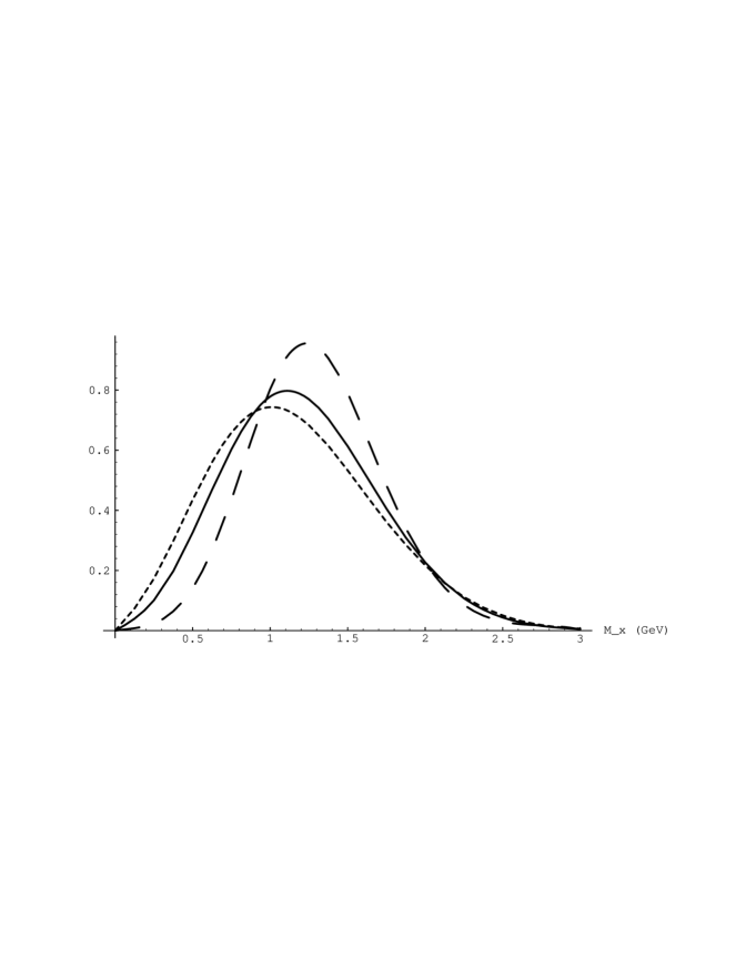
Figure 3: Dependence of $d\Gamma/dM_{x}$ on $\mu_{\pi}^{2}$: long-dashed, solid, and short-dashed lines correspond to $\tilde{\mu}_{\pi}^{2}=0.2\,\mbox{GeV}^{2}$, $0.4\,\mbox{GeV}^{2}$ and $0.6\,\mbox{GeV}^{2}$. The $b$-quark mass $\tilde{m}_{b}=4.82\,\mbox{GeV}$, $\alpha_{s}=0.3$. All distributions are normalized to the same total width.

There is a third consideration to be elaborated now. Since the recoil spectrum is shaped by nonperturbative dynamics, it is sensitive to the values of $\tilde{m}_{b}$ and $\tilde{\mu}_{\pi}^{2}$. Varying $\tilde{\mu}_{\pi}^{2}$ between $0.2$ and $0.6\,\mbox{GeV}^{2}$ while keeping $\alpha_{s}=0.3$ and $\tilde{m}_{b}=4.82\,\mbox{GeV}$ fixed one obtains the three curves of Figs. 3 and 4. Changing $\tilde{m}_{b}$ between $4.77$ and $4.87\,\mbox{GeV}$, one obtains a somewhat larger difference in the spectrum – as shown in Figs. 5 and 6. With abundant statistics one can, in principle, distinguish the different curves and try to extract $m_{b}$ and $\mu_{\pi}^{2}$ – in addition to $|V_{ub}|$. Yet it will take some time before such statistics become available. Realistically, we expect here only a cross-check of the consistency with other, dedicated experimental evaluations of these parameters.

In the meantime one can quite profitably concentrate on analyzing $\Phi(M_{\rm max})$, with the primary goal placed on determining $|V_{ub}|$. Since the theoretical uncertainty in the total width $\Gamma_{\rm sl}(b\rightarrow u)$ or in the ratio $\Gamma_{\rm sl}(b\rightarrow u)/\Gamma_{\rm sl}(b\rightarrow c)$ is small and depends on different type of effects, we dwell now on the uncertainty of predicting the rate in the kinematics where $b\rightarrow u$ decays can be experimentally disentangled from the KM-allowed transitions. In other words, we must understand how accurately one can calculate theoretically $\Phi(M_{\rm max})$ for realistic values of the cutoff mass $M_{\rm max}$. The first step is clearly to analyze its dependence on not yet precisely known parameters of the heavy quark expansion.

In Fig. 4 the predictions are plotted as a function of $M_{\rm max}$ for the three values $\tilde{\mu}_{\pi}^{2}=0.2,\;0.4,\;0.6\,\mbox{GeV}^{2}$ with $\tilde{m}_{b}=4.82\,\mbox{GeV}$ fixed and in Fig. 6 for $\tilde{m}_{b}=4.78\,\mbox{GeV},\;4.82\,\mbox{GeV}$ and $4.87\,\mbox{GeV}$ with $\tilde{\mu}_{\pi}^{2}=0.4\,\mbox{GeV}^{2}$ fixed. We see immediately that the lower $M_{\rm max}$ is chosen, the higher the sensitivity to long-distance dynamics becomes. This is not surprising qualitatively since for a lower $M_{\rm max}$ a smaller fraction of the overall rate is included.

The intervals of variation for $m_{b}$ and $\mu_{\pi}^{2}$ we consider are quite conservative. The actual existing uncertainty in the latter seems to be $1.5$–$2$ times smaller [1]; it is hardly possible that the $b$ quark mass entering our calculations can vary in a wider interval. Taking for orientation $M_{\rm max}=1.5$ to $1.6\,\mbox{GeV}$ we observe that the dependence of the fraction of the events $\Phi\left(M_{\rm max}\right)$ on $m_{b}$ is more pronounced. To illustrate this dependence more clearly, we give the exploded version of Figs. 5 and 6 in Figs. 7 and 8 where we vary $m_{b}$ by twice larger amount $\pm 100\,\mbox{MeV}$. The variation in the fraction of the events remains reasonably small for $M_{\rm max}\mathrel{\hbox to0.0pt{\lower 4.0pt\hbox{\hskip 1.0pt$\sim$}\hss}\raise 1.0pt\hbox{$>$}}1.6\,\mbox{GeV}$.

The stability deteriorates when one descends already a few hundred  MeV below. One not only loses statistics, the fraction $\Phi$ becomes essentially dependent on the nonperturbative parameters.

Thus we see that the goals of larger statistics and smaller sensitivity to nonperturbative effects favor the selection of as high a value for $M_{\rm max}$ as experimentally feasible, considering leakage from $b\rightarrow c$.

To be more specific: taking the plots literally, about $70\%$ of all $b\rightarrow u$ events lie below $M_{\rm max}=1.5\,\mbox{GeV}$ with a spread of $\pm 8$%; for $M_{\rm max}=1.3\,\mbox{GeV}$ and $1.0\,\mbox{GeV}$ these numbers read $\simeq 60\%$ and $\simeq 35\%$, respectively, with a spread of $\pm 12\%$ and $\pm 15\%$, respectively. These are uncertainties on top of those for the total $B\rightarrow l\nu X_{u}$ width listed in Eq. (3) which are encountered in converting the semileptonic width into $|V_{ub}|$. For $M_{\rm max}\mathrel{\hbox to0.0pt{\lower 3.0pt\hbox{\hskip 0.0pt$\sim$}\hss}\raise 1.0pt\hbox{$<$}}1.5\,\mbox{GeV}$ the uncertainties in the width pale in comparison to those due to the shape of spectrum.

In reality, one must allow for additional uncertainties associated with other approximations made in the analysis; most profoundly, the effect of the subleading nonperturbative effects in the structure functions not captured by naive Fermi motion is quite non-negligible for the actual $b$ quark mass. Their theoretical discussion and the estimate of related uncertainty can be found in [14, 16]. As long as one does not aim for an absolute precision in $\Phi(M_{\rm max})$ below $\sim 10\%$, they are not expected to be important. Nonetheless, additional work toward better control of remaining uncertainties is clearly needed. Without a doubt, it will receive necessary theoretical attention as soon as the experimental feasibility of such measurements will be established and their ultimate precision is understood.

4 Summary and Outlook

We have shown here that if one succeeds in measuring the hadronic recoil mass spectrum in semileptonic $B$ decays, one can extract $|V_{ub}|$ in a theoretically clean and accurate way. In our theoretical analysis we split the problem into two parts – one is calculating the overall semileptonic $b\rightarrow u$ width of $B$ mesons, and the second is determining the fraction of $b\rightarrow u$ events that can be discriminated kinematically against $b\rightarrow c$ processes. A good theoretical control over the first theoretical ingredient allowed us to concentrate on the more subtle second aspect.

Perturbative as well as nonperturbative QCD dynamics have a large impact on the mass spectrum – they broaden it considerably. Yet the numerical analysis suggests that they do not change very much one basic feature, namely that only a small tail distribution extends beyond $M_{D}$. Furthermore, while the shape of the spectrum is sensitive to long-distance dynamics, its integrated weight, say below $1.5\,\mbox{GeV}$ is much less so. There is nothing magic about the value of $1.5\,\mbox{GeV}$. What is important is that one selects a cut-off that is high enough for most of the $b\rightarrow u$ transitions to contribute below and low enough for almost all $b\rightarrow c$ leakage to occur above. Nevertheless, not only statistics, but also the issue of theoretical reliability calls for attempts to set as high a cut-off as possible.

Thus the following scenario emerges: measuring the semileptonic decay rate below, say, $M_{\rm max}=1.5\,\mbox{GeV}$ will enable us to extract $|V_{ub}|$ with a theoretical uncertainty that does not exceed $10\>$–$\>20$ percent. An overall uncertainty of below $10\%$ appears achievable or at least not impossible since with $10^{7}-10^{8}$ $B$ decays and ${\rm BR}(B\rightarrow l\nu X_{u})\simeq 0.0015$ one estimates that a statistical accuracy level $\sim{\cal O}(1\%)$ would be available, provided a large fraction of the decay events can be successfully utilized. As described above, a particular premium above and beyond statistics has to be placed on achieving a high value for $M_{\rm max}$, not below $1.5\,\mbox{GeV}$.

Meanwhile, if the studies will demonstrate the feasibility of such experimental measurements, the theoretical description can be improved. The feasible method of obtaining accurate perturbative corrections to the decay structure functions was suggested in [14], the so-called APS which combined advantages of exact one loop-expressions, exponentiation of soft infrared/collinear effects and incorporating of the running of the coupling. It intrinsically includes the normalization point and thus is free of problems associated with using the pole mass of $b$ quark encountered in the “practical” OPE. Yet for the reasons elucidated above we do not anticipate qualitative changes in our predictions. In particular, the resummation of next-to-leading logs does not seem very promising in the semileptonic decays due to a limited gap in the momentum scales. Without a cutoff, however, the resummation of leading logs seems technically necessary not to violate unitarity for soft emissions. It is important to check that the sensitivity to the exact treatment of the perturbative corrections is not high, since application of the perturbative expansion at a precise level for the soft gluons with $M_{x}\mathrel{\hbox to0.0pt{\lower 3.0pt\hbox{\hskip 0.0pt$\sim$}\hss}\raise 1.0pt\hbox{$<$}}1\,\mbox{GeV}$ seems problematic.

In the near future one will presumably determine $m_{b}$ and $\mu_{\pi}^{2}$ from $b\rightarrow c$ transitions with even better accuracy than stated above. Lastly, with increasing statistics one can measure the $b\rightarrow u$ recoil mass spectrum with good accuracy, rather than its integral as a function of $M_{\rm max}$. This in turn will allow us to independently place bounds on $m_{b}$ and $\mu_{\pi}^{2}$ in a systematic way. Comparing these bounds with other determinations of these basic quantities will serve as an essential quality check on systematic uncertainties and the quantitative applicability of the heavy quark expansion.

If accurate measurements of the recoil mass spectrum are feasible at all, it is advantageous to perform such studies separately for charged and neutral $B$. In the KM-suppressed semileptonic decays one can observe the effects of Weak Annihilation as the difference in the decay characteristics for charged and neutral $B$. Moreover, in the decays to massless leptons one is sensitive to the nonfactorizable parts of the expectation values of the four-quark operators responsible for the effects of Weak Annihilation [17]. On the other hand, it is just the theoretical expectations for nonfactorizable parts which are a subject of some controversy in the literature at the moment. Gaining direct experimental information not only can put theoretical predictions of beauty lifetimes on more solid grounds, but also has an independent theoretical interest. Ultimately, Weak Annihilation can even introduce an element of theoretical uncertainty in the extraction of $|V_{ub}|$ in the discussed way unless its effect is controlled through such studies.

At the same time, theoretically, the effects of Weak Annihilation are expected to come from small $M_{X}$ (or even from small hadronic recoil energy $E_{h}$) [17]; singling out this domain can amplify the effect and make it detectable even if its overall scale is insignificant.
Acknowledgments:    After publication of paper [16] where the QCD-based analysis of the recoil mass distribution was first reported, along with other decay distributions, a paper by Falk, Ligeti and Wise appeared [19] which discussed the similar issue of extracting $|V_{ub}|$ from the recoil mass spectrum. R. Dikeman would like to thank B. Urbanski for her generous hospitality during the completion of this work. Our work was supported in part by the National Science Foundation under the grant number PHY 92-13313 and by DOE under the grant number DE-FG02-94ER40823.

Figure 1: Effect of radiative corrections on $d\Gamma/dM_{x}$: solid line shows $\alpha_{s}=0.3$, dashed and dotted lines are $\alpha_{s}=0.1$ and $\alpha_{s}=0.5\,$, respectively. $\tilde{m}_{b}=4.82\,\mbox{GeV}$ and $\tilde{\mu}_{\pi}^{2}=0.4\,\mbox{GeV}^{2}$.

Figure 2: The integrated fraction of the events $\Phi(M_{x})$.

Figure 4: $\Phi(M_{x})$ for $\tilde{\mu}_{\pi}^{2}=0.2\,\mbox{GeV}^{2}$, $0.4\,\mbox{GeV}^{2}$ and $0.6\,\mbox{GeV}^{2}$.

Figure 5: Dependence of $d\Gamma/dM_{x}$ on $m_{b}$: long-dashed, solid, and short-dashed lines are $\tilde{m}_{b}=4.77\,\mbox{GeV}$, $4.82\,\mbox{GeV}$ and $4.87\,\mbox{GeV}$. $\tilde{\mu}_{\pi}^{2}=0.4\,\mbox{GeV}^{2}$, $\alpha_{s}=0.3$.

Figure 6: $\Phi(M_{x})$ in the same setting as in Fig. 5.

Figure 7: $d\Gamma/dM_{x}$ for $\tilde{m}_{b}=4.72\,\mbox{GeV}$, $4.82\,\mbox{GeV}$ and $4.92\,\mbox{GeV}$. $\tilde{\mu}_{\pi}^{2}=0.4\,\mbox{GeV}^{2}$, $\alpha_{s}=0.3$.

Figure 8: $\Phi(M_{x})$ in the same setting as in Fig. 7.

References

- [1] I.I. Bigi, M.Shifman, N. Uraltsev, preprint hep-ph/9703290, with references to earlier works.
- [2] A. Ali, E. Pietarinen Nucl. Phys. B154 (1979) 519.
- [3] G. Altarelli et al., Nucl. Phys. B208 (1982) 365.
- [4] I. Bigi, M. Shifman, N.G. Uraltsev, A. Vainshtein, Phys. Rev. Lett. 71 (1993) 496.
- [5] I. Bigi, M. Shifman, N.G. Uraltsev and A. Vainshtein, Phys. Lett. B328 (1994) 431.
- [6] For a recent review see [1]; the details of the QCD descriptions of the “Fermi motion” in beauty decays can be found in the dedicated papers [11, 14] and other publications [15] referred to there.
- [7] I. Bigi, N.G. Uraltsev and A. Vainshtein, Phys. Lett. B293 (1992) 430; (E) B297 (1993) 477.
-
[8]
B. Blok, R. Dikeman and M. Shifman, Phys. Rev. D51
(1995) 6167;
M. Gremm and A. Kapustin, hep-ph/9603448. - [9] N.G. Uraltsev, Int. Journ. Mod. Phys. A11 (1996) 515.
- [10] V. Barger, C.S. Kim, G.J.N. Phillips, Phys. Lett. B251 (1990) 629.
- [11] I. Bigi, M. Shifman, N. Uraltsev, A. Vainshtein, Int. Journ. Mod. Phys. A9 (1994) 2467.
- [12] B. Blok, L. Koyrakh, M. Shifman, A. Vainshtein, Phys. Rev. D49 (1994) 3356.
- [13] I. Bigi, M. Shifman, N. Uraltsev, A. Vainshtein, Phys. Rev. D52 (1995) 196.
- [14] R.D. Dikeman, M. Shifman and N.G. Uraltsev, Int. Journ. Mod. Phys., A11 (1996) 571.
-
[15]
R. Jaffe and L. Randall, Nucl. Phys. B412 (1994) 79
A. Falk, E. Jenkins, A. Manohar and M. Wise, Phys. Rev. D49 (1994) 4553;
M. Neubert, Phys. Rev. D49 (1994) 4623. - [16] R.D. Dikeman and N.G. Uraltsev, preprint hep-ph/9703437.
- [17] I. Bigi and N. Uraltsev, Nucl. Phys. B423 (1994) 33.
- [18] C. Greub, S.-J. Rey, Preprint SLAC-PUB-7245 [hep-ph 9608247], Eq. (17).
- [19] A. Falk, Z. Ligeti and M. Wise, preprint hep-ph/9705235.