MPI-Ph/97-015 DESY 97-119
TUM-HEP-274/97 hep-ph/9706501

Penguin Diagrams, Charmless B-Decays and the
“Missing Charm Puzzle”
Alexander Lenz,
Max-Planck-Institut für Physik — Werner-Heisenberg-Institut,
Föhringer Ring 6, D-80805 München, Germany,
Ulrich Nierste,
DESY - Theory group, Notkestrasse 85, D-22607 Hamburg, Germany,
and
Gaby Ostermaier
Physik-Department, TU München, D-85747 Garching, Germany

Abstract

We calculate the contributions of penguin diagrams with internal $u$ or $c$ quarks to various inclusive charmless B-decay rates. Further we analyze the influence of the chromomagnetic dipole operator $Q_{8}$ on these rates. We find that the rates corresponding to $\overline{B}\rightarrow X_{u\overline{u}s}$, $\overline{B}\rightarrow X_{d\overline{d}s}$, $\overline{B}\rightarrow X_{s\overline{s}s}$, $\overline{B}\rightarrow X_{s\overline{s}d}$ and $\overline{B}\rightarrow X_{d\overline{d}d}$ are dominated by the new penguin contributions. The contributions of $Q_{8}$ sizably diminish these rates. Despite of an increase of the total charmless decay rate by 36 % the new contributions are not large enough to explain the charm deficit observed by ARGUS and CLEO. We predict $n_{c}=1.33\pm 0.06$ for the average number of charmed particles per B-decay in the Standard Model. Then the hypothesis of an enhancement of the chromomagnetic dipole coefficient $C_{8}$ by new physics contributions is analyzed. We perform a model independent fit of $C_{8}$ to the experimental data. If the CKM structure of the new physics contribution is the same as in the Standard Model, $|C_{8}(M_{W})|$ must be enhanced by a factor of 9 to 16 in order to explain the observed charm deficit.

1 Introduction

Precision measurements performed at the $\Upsilon(4S)$ resonance find less charmed particles in the final states of B meson decays than theoretically expected. The CLEO 1.5, CLEO II and ARGUS data give [1]

$$n^{\mathit{exp}}_{c}\;=\;1.15\pm 0.05$$ (1)

for the average number of charm (anti-)quarks per B⁺/B⁰-decay. Complementary information on inclusive B decays can be obtained from the semileptonic branching ratio. The CLEO and ARGUS groups [1, 2] have measured

$$B^{\mathit{exp}}_{SL} = 10.23\pm 0.39\%.$$ (2)

The increasing experimental precision achieved in the current decade has been paralleled by a substantial progress in the theoretical understanding of the inclusive decay rates entering $B_{SL}$ and $n_{c}$. Here the calculational key is the heavy quark expansion (HQE) [3, 4] of the decay rate in question: The leading term of the HQE reproduces the decay rate of a b-quark in the QCD-corrected parton model. The first non-perturbative corrections are suppressed by a factor of $(\Lambda_{QCD}/m_{b})^{2}$ and affect the rates by at most a few percent. Theoretically spectator effects of order $16\pi^{2}(\Lambda_{QCD}/m_{b})^{3}$ [5, 6] could be larger [6], but for the decay rates of B^± and B⁰ entering (2) and (1) they are experimentally known to be at the percent level as well [7]. The apparent smallness of these non-perturbative terms has shifted the focus towards the perturbative corrections to the free quark decay. The calculation of such short distance effects starts from an effective hamiltonian, whose generic form reads

$$H = \frac{G_{F}}{\sqrt{2}}\left[V_{\mathit{CKM}}\sum_{j=1}^{2}C_{j}Q_{j}-V_{\mathit{CKM}}^{\prime}\left(\sum_{k=3}^{6}C_{j}Q_{j}+C_{8}Q_{8}\right)\right].$$ (3)

Here $G_{F}$ is the Fermi constant and $V_{\mathit{CKM}}$ and $V_{\mathit{CKM}}^{\prime}$ are products of elements of the Cabibbo-Kobayashi-Maskawa (CKM) matrix. The Wilson coefficients $C_{j}$ encode the physics connected to the weak scale and play the rôle of effective coupling constants of the local interactions described by the operators $Q_{j}$. Their precise form depends on the flavour structure of the decay and will be given below in (14).

Decays with three different flavours in the final state such as $b\rightarrow c\overline{u}d$ can only proceed through the current-current operators $Q_{1}$ and $Q_{2}$. $\Gamma(b\rightarrow c\overline{u}d)$ has been calculated to order $\alpha_{s}$, which is the next-to-leading order (NLO), in [8]. The generic Feynman diagram for these corrections are depicted in Fig. 3. In [9] the same diagrams have been calculated for $\Gamma(b\rightarrow c\overline{c}s)+\Gamma(b\rightarrow c\overline{c}d)$. The latter decays and the charmless nonleptonic decays, however, also involve penguin effects. Diagrams with insertions of the penguin operators $Q_{3-6}$ have been taken into account only in the leading order (LO) [10, 9, 11], because their coefficients $C_{3-6}$ are much smaller than $C_{1,2}$ (cf. Tab. 1). The results for $B_{SL}$ and $n_{c}$ read

$$B_{SL}=\left(11.7\pm 1.4\pm 1.0\right)\%,\qquad n_{c}=1.34\mp 0.06.$$ (4)

Here the result for $B_{SL}$ has been obtained in [10, 12] with the analytical input from [8, 10, 9]. The second error bar has been added to account for the spectator effects estimated in [6]. Apparently there is no spectacular discrepancy between (2) and (4). The result for $n_{c}$ in (4) does not involve the calculation of $\Gamma(b\rightarrow c\overline{c}d)+\Gamma(b\rightarrow c\overline{c}s)$, but instead uses the experimental information on $B_{SL}$ in (2) as proposed in [13, 14]. We discuss this in more detail in sect. 2.

The discrepancy between (1) and (4) constitutes the “missing charm puzzle”. The search for a theoretical explanation has recently focused on new positive contributions to the yet unmeasured charmless decay modes entering (4). Indeed, in a recent analysis [14] $\Gamma(b\rightarrow\textit{no charm})$ has been estimated indirectly in two different ways: First the experimental information on final states with hadrons containing a $c$ quark has been used and second data on decay products involving a $\overline{c}$ quark have been analyzed. For the CLEO data both methods consistently indicate an enhancement of $\Gamma(b\rightarrow\textit{no charm})$ by roughly a factor of 14 compared to the theoretical prediction in [11].

Next we briefly discuss the LEP results for $B_{SL}$ and $n_{c}$ [15]. The LEP Z-peak experiments encounter a mixture of b-flavoured hadrons. In order to allow for a comparison with (2) one must correct the LEP result $B^{\mathit{Z,exp}}_{SL}=10.95\pm 0.42\%$ [1] for the different lifetimes [7] of the hadrons in the mixture [16]:

$$B^{\mathit{Z,corr,exp}}_{SL} = 11.13\pm 0.42\%,\qquad\qquad\qquad n_{c}^{\mathit{Z,exp}}\;=\;1.22\pm 0.08.$$ (5)

These data are consistent with the theory (cf. (9) below), but the analysis in [14] has found evidence for an enhanced $\Gamma(b\rightarrow\textit{no charm})$ also from the LEP data. Further the two methods used in [14] have given less consistent results for the LEP data than for the CLEO data. In addition the LEP measurements involve the $\Lambda_{b}$ baryon, whose lifetime is either not properly understood theoretically or incorrectly measured. (If the latter is the case, $B^{\mathit{Z,corr,exp}}_{SL}$ in (5) must be replaced by the uncorrected $B^{\mathit{Z,exp}}_{SL}$, which reduces the $2\sigma$ discrepancy between (2) and (5).) Hence in our analysis we will mainly use (2) and (1).

Now two possible sources of an enhanced $\Gamma(b\rightarrow\textit{no charm})$ are currently discussed: The authors of [17] stress the possibility that the Wilson coefficient $C_{8}$ of the chromomagnetic dipole operator $Q_{8}$ is enhanced by new physics contributions. On the other hand in [14, 18] an explanation within QCD dynamics is suggested: An originally produced $(c,\overline{c})$-pair can annihilate and thereby lead to a charmless final state.

The calculation of matrix elements involving $Q_{3-6}$ and $Q_{8}$ does not exhaust all possible penguin effects. In this paper we calculate the contributions of penguin diagrams with insertions of the current-current operator $Q_{2}$ to the decay rates into charmless final states (see Fig. 3). Such a penguin diagram with a $(c,\overline{c})$-pair in the intermediate state involves the large coefficient $C_{2}$ and the CKM factor $V_{cb}\gg|V_{ub}|$. It is precisely the short distance analogue of the mechanism proposed in [14, 18] and surprisingly has not been considered in the perturbative calculations [9, 10, 11, 20] of the decay rates entering $B_{SL}$ and $n_{c}$.

Further we calculate the diagrams involving the interference of the tree diagram with $Q_{8}$ in Fig. 3 with $Q_{1-6}$, which belongs to the order $\alpha_{s}$ as well. The consideration of these diagrams is mandatory, if one wants to estimate the effect of an enhanced coefficient $C_{8}$ on $\Gamma(b\rightarrow\textit{no charm})$ proposed in [17].

The paper is organized as follows: In the following section we set up our notations and collect results from earlier work. The calculation of the penguin diagram contributions and the $Q_{1-6}$–$Q_{8}$ interference terms is presented in sect. 3. The phenomenologically interested reader is refered to sect. 4, in which we discuss our numerical results. In sect. 4 we also comment on the mechanism proposed in [18]. Further a potential enhancement of $C_{8}$ is analyzed by a model independent fit of $C_{8}$ to the experimental data. Finally we conclude.

 

Figure 1: Example of a current-current diagram. The cross denotes the inserted operator. $d^{\prime}$ equals $d$ or $s$.

Figure 2: Penguin diagram involving $Q_{2}$. The internal quark $q^{\prime}$ can be $u$ or $c$. The corresponding diagram with $Q_{1}$ vanishes.

Figure 3: Tree diagram contribution of $Q_{8}$ to $\Gamma(b\rightarrow q\overline{q}d^{\prime})$.

 

2 Preliminaries

2.1 $\mathbf{B_{SL}}$ and $\mathbf{n_{c}}$

For the theoretical description of the various decay rates it is advantageous to normalize them to the well-understood semileptonic decay rate [13, 14]:

$$\!\!\!r_{q\ell}=\frac{\Gamma\left(\overline{B}\rightarrow X_{q}\ell\overline{\nu}_{\ell}\right)}{\Gamma\left(\overline{B}\rightarrow X_{c}e\overline{\nu}_{e}\right)},\qquad r_{q_{1}\overline{q_{2}}q_{3}}\! = \!\frac{\Gamma\left(\overline{B}\rightarrow X_{q_{1}\overline{q_{2}}q_{3}}\right)}{\Gamma\left(\overline{B}\rightarrow X_{c}e\overline{\nu}_{e}\right)},\qquad r_{qg}=\frac{\Gamma\left(\overline{B}\rightarrow X_{qg}\right)}{\Gamma\left(\overline{B}\rightarrow X_{c}e\overline{\nu}_{e}\right)}.$$ (6)

This eliminates the factor of $m_{b}^{5}$ common to all decay rates. For the charmless decays we will further use

$$r_{c/} = \sum_{\scriptstyle q=d,s\atop\scriptstyle q^{\prime}=u,d,s}\left[r_{q^{\prime}\overline{q}^{\prime}q}+r_{qg}\right]+2r_{ue}.$$ (7)

The semileptonic branching ratio reads

$$B_{SL} = \frac{1}{2+r_{c\tau}+r_{c/}+\sum_{q=d,s}\left[r_{c\overline{u}q}+r_{c\overline{c}q}\right]}.$$ (8)

Small contributions such as $r_{u\tau}=0.004$ and radiative decay modes have been omitted in (7). In (8) also $r_{u\overline{c}s}=0.05$ [11] has been neglected. The numerical value for $B_{SL}$ in (4) is the average of the two results given in [10] corresponding to two different renormalization schemes (on-shell vs. $\overline{\rm MS}$ [21] quark masses). In the corresponding expression for $n_{c}$ the term $r_{c\overline{c}s}+r_{c\overline{c}d}$, which suffers from sizeable theoretical uncertainties, is eliminated in favour of $B_{SL}$ [13, 14]:

$$n_{c} = 2-\left(2+r_{c\tau}+r_{c\overline{u}d}+r_{c\overline{u}s}+2r_{c/}\right)B_{SL}.$$ (9)

Yet with [8, 22]

$$r_{c\overline{u}s}+r_{c\overline{u}d}\;=\;4.0\pm 0.4, \qquad r_{c\tau}\;=\;0.25$$ (10)

and $B^{\mathit{exp}}_{SL}$ in (2) one obtains

$$n_{c} = 1.36\mp 0.04\,-\,0.205\cdot r_{c/}.$$ (11)

Now the current-current type radiative corrections to $r_{c/}$ (cf. Fig. 3) have been calculated in [20, 23, 8] using different renormalization schemes. The penguin operators $Q_{3-6}$ have been included within the LO in [11]. With up-to-date values for $B_{SL}$ and the CKM elements the calculation of [11] yields $r_{c/}=0.11\pm 0.08$. Inserting this result into (11) yields the numerical value in (4). In contrast the indirect experimental determination in [14] has found $r_{c/}=1.6\pm 0.4$. In order to reproduce the experimental value of $n_{c}$ in (1) one needs $r_{c/}=1.0\pm 0.4$.

So far the penguin diagrams of Fig. 3 have not been calculated for all possible charmless B decay modes. Yet for the pure penguin induced decays of a $b$-quark into three down-type (anti)-quarks the contribution of the diagram of Fig. 3 has been obtained in terms of a twofold integral representation in [19]. Likewise the effect of penguin diagrams on the analysis of CP asymmetries has been studied in [19, 24] and in [25] penguin effects on exclusive decays have been studied.

2.2 Decay rates to order $\alpha_{s}$

In order to describe decays of the type $b\rightarrow q\overline{q}d$ one needs the following hamiltonian:

$$H = \frac{G_{F}}{\sqrt{2}}\left\{\sum_{j=1}^{2}C_{j}\left(\xi_{c}^{*}Q_{j}^{c}+\xi_{u}^{*}Q_{j}^{u}\right)-\xi_{t}^{*}\sum_{j\in\mathcal{P}}C_{j}Q_{j}\right\}\;,\qquad\qquad\xi_{q^{\prime}}\;=\;V_{q^{\prime}b}^{*}V_{q^{\prime}d}\;.$$ (12)

Here $\xi_{u}+\xi_{c}+\xi_{t}=0$ due to the unitarity of the CKM matrix and $\mathcal{P}=\{3,\ldots 6,8\}$. $H$ in (12) comprises the following operator basis:

$$\left.\begin{array}[]{@{\hspace{-14em}}rcl}Q_{1}^{q}&=&(\bar{d}q)_{V-A}\cdot(\bar{q}b)_{V-A}\cdot\widetilde{\leavevmode\hbox{\small 1\kern-3.8pt\normalsize 1}}\\[2.84526pt] Q_{2}^{q}&=&(\bar{d}q)_{V-A}\cdot(\bar{q}b)_{V-A}\cdot\leavevmode\hbox{\small 1\kern-3.8pt\normalsize 1}\\ \end{array}\right\}\quad\textrm{with $q=u$ or $q=c$,}$$

$$Q_{3}^{q}\;=\;(\bar{d}b)_{V-A}\cdot(\bar{q}q)_{V-A}\cdot\leavevmode\hbox{\small 1\kern-3.8pt\normalsize 1}, \qquad Q_{4}^{q}\;=\;(\bar{d}b)_{V-A}\cdot(\bar{q}q)_{V-A}\cdot\widetilde{\leavevmode\hbox{\small 1\kern-3.8pt\normalsize 1}}$$

$$Q_{5}^{q}\;=\;(\bar{d}b)_{V-A}\cdot(\bar{q}q)_{V+A}\cdot\leavevmode\hbox{\small 1\kern-3.8pt\normalsize 1}, \qquad Q_{6}^{q}\;=\;(\bar{d}b)_{V-A}\cdot(\bar{q}q)_{V+A}\cdot\widetilde{\leavevmode\hbox{\small 1\kern-3.8pt\normalsize 1}}$$

$$Q_{j}\;=\;\sum_{q=u,d,s,c,b}Q_{j}^{q}\hskip 60.00009pt 3\leq j\leq 6$$ for ,

$$Q_{8}\;=\;-\frac{g}{8\pi^{2}}\,\bar{d}\sigma^{\mu\nu}\left[m_{d}L+m_{b}R\right]T^{a}b\cdot G^{a}_{\mu\nu}\;.$$ (14)

The colour singlet and non-singlet structure are indicated by 11 and $\widetilde{\leavevmode\hbox{\small 1\kern-3.8pt\normalsize 1}}$ and $V\pm A$ is the Dirac structure, i.e.

$$\left(\bar{d}q\right)_{V-A}\cdot\left(\bar{q}b\right)_{V-A}\cdot\widetilde{\leavevmode\hbox{\small 1\kern-3.8pt\normalsize 1}} = \bar{d}_{\alpha}\gamma_{\mu}\left(1-\gamma_{5}\right)q_{\beta}\cdot\bar{q}_{\beta}\gamma^{\mu}\left(1-\gamma_{5}\right)b_{\alpha}.$$

Next it is useful to expand the renormalized matrix elements in $\alpha_{s}$ and to separate the result from current-current diagrams (see Fig. 3) and penguin diagrams (see Fig. 3):

$$\langle\,q\overline{q}d\,|Q_{j}^{q^{\prime}}|\,b\,\rangle = \langle\,Q_{j}^{q^{\prime}}\,\rangle^{(0)}+\frac{\alpha_{s}}{4\pi}\left[\langle\,Q_{j}^{q^{\prime}}\,\rangle^{(1)}_{\mathit{cc}}+\langle\,Q_{j}^{q^{\prime}}\,\rangle^{(1)}_{\mathit{peng}}\right]+O(\alpha_{s}^{2}),\qquad j=1,2,$$ (15)

$$\langle\,Q_{j}^{q^{\prime}}\,\rangle^{(1)}_{\mathit{peng}} = \sum_{k\in\mathcal{P}}r^{q^{\prime}}_{jk}\left(p^{2},m_{q^{\prime}},\mu\right)\langle Q_{k}\rangle^{(0)},\qquad\qquad\qquad p=p_{b}-p_{d}\;.$$ (16)

Of course $\langle\,Q_{j}^{q^{\prime}}\,\rangle^{(0)}$ and $\langle\,Q_{j}^{q^{\prime}}\,\rangle^{(1)}_{\mathit{cc}}$ are non-zero only for $q=q^{\prime}=u$, recall that we do not consider $q=c$ in this work. In (16) we have expressed the result of the penguin diagram in terms of the tree-level matrix elements. There $\mu$ is the renormalization scale. For the momentum flow cf. Fig. 3.

The quark decay rate is related to the matrix element of $H$ via

$$\Gamma\left(b\rightarrow q\overline{q}d\right) = \frac{1}{2m_{b}}\!\int\!\!\frac{d^{3}\vec{p}_{q}d^{3}\vec{p}_{\bar{q}}d^{3}\vec{p}_{d}}{(2\pi)^{5}8|E_{q}E_{\bar{q}}E_{d}|}\delta^{(4)}\left(p_{b}+p_{\bar{q}}-p_{q}-p_{d}\right)\overline{\langle\,q\overline{q}d\,|H|\,b\,\rangle\langle\,q\overline{q}d\,|H|\,b\,\rangle^{*}}.$$

The bar over $\langle\,q\overline{q}d\,|H|\,b\,\rangle\langle\,q\overline{q}d\,|H|\,b\,\rangle^{*}$ denotes the average over initial state polarizations and the sum over final state polarizations. Next we expand the decay rate to order $\alpha_{s}$:

$$\Gamma\left(b\rightarrow q\overline{q}d\right) = \Gamma^{(0)}+\frac{\alpha_{s}(\mu)}{4\pi}\left[\Delta\Gamma_{\mathit{cc}}+\Delta\Gamma_{\mathit{peng}}+\Delta\Gamma_{8}+\Delta\Gamma_{\mathit{W}}\right]+O(\alpha_{s}^{2}).$$ (17)

For $b\rightarrow q\overline{q}s$ decays one simply substitutes $d$ by $s$ in (14-17). Now the first two terms of the NLO correction in (17) describe the effect of current-current and penguin diagrams involving $Q_{1}$ or $Q_{2}$. $\Delta\Gamma_{8}$ likewise contains the matrix elements of $Q_{8}$. The remaining part $\Delta\Gamma_{W}$ of the NLO contribution is made of the corrections to the Wilson coefficients [20, 28] multiplying the tree-level amplitudes in $\Gamma^{(0)}$. We write

$$C_{j}(\mu) = C_{j}^{(0)}(\mu)+\frac{\alpha_{s}(\mu)}{4\pi}\Delta C_{j}(\mu),\qquad\qquad j=1,\ldots 6.$$ (18)

Here $\Delta C_{j}$ is the NLO correction to the Wilson coefficient. $\Delta C_{j}$ depends on the renormalization scheme chosen. This scheme dependence cancels with a corresponding one in the results of the loop diagrams contained in $\Delta\Gamma_{cc}$ and $\Delta\Gamma_{peng}$. For example the scheme dependence of $\Delta C_{1,2}$ cancels in combination with the current-current type corrections to $Q_{1}$ and $Q_{2}$ of Fig. 3. Since we do not include the unknown radiative corrections to the penguin operators $Q_{3-6}$ in (17), we must likewise leave out terms in $\Delta C_{j}$ related to the NLO penguin-penguin mixing in order to render $\Gamma$ in (17) scheme independent. We ban these technical details into the appendix. The values of the Wilson coefficients needed for the numerical evaluation of the various decay rates are listed in Tab. 1.

 

j	1	2	3	4	5	6	8
$C_{j}^{(0)}(\mu=m_{b})$	-0.2493	1.1077	0.0111	-0.0256	0.0075	-0.0315	-0.1495
$C_{j}^{NDR}(\mu=m_{b})$	-0.1739	1.0731	0.0113	-0.0326	0.0110	-0.0384
$C_{j}^{(0)}(\mu=m_{b}/2)$	-0.3611	1.1694	0.0170	-0.0359	0.0100	-0.0484	-0.1663
$C_{j}^{NDR}(\mu=m_{b}/2)$	-0.2720	1.1246	0.0174	-0.0461	0.0149	-0.0587
$C_{j}^{(0)}(\mu=2\,m_{b})$	-0.1669	1.0671	0.0071	-0.0176	0.0054	-0.0202	-0.1355
$C_{j}^{NDR}(\mu=2\,m_{b})$	-0.1001	1.0389	0.0073	-0.0227	0.0079	-0.0251
$\Delta\overline{C}_{j}(\mu=m_{b})$	2.719	-1.744	0.380	-0.1050	-0.223	0.384

Table 1: Wilson coefficients used in our analysis. $C_{j}^{(0)}$ is the LO expression, $C_{j}^{NDR}$ is the NLO coefficient in the NDR scheme. In $C_{j}^{NDR}$ above the NLO corrections to penguin-penguin mixing have been omitted in order to render $\Gamma$ in (33) scheme independent as described in the text. For $\mu=m_{b}$ this affects $C_{3}$ and $C_{5}$ by 12 % and 25 %, but is negligible for the other coefficients. $C_{j}^{(0)}$ and $C_{j}^{NDR}$ are needed for the numerical evaluation of the decay rate in (33). $\Delta\overline{C}_{j}$ in the last line is defined in (56). The top and bottom mass are chosen as $m_{t}=m_{t}^{\overline{\mathrm{MS}}}(m_{t})=168$ GeV and $m_{b}=4.8$ GeV. Further $\alpha_{s}(M_{Z})=0.118$ [29], which corresponds to $\alpha_{s}(4.8\mathrm{GeV})=0.216$. In the table $C_{8}^{(0)}=C_{8}^{(0),eff}$ is the scheme independent coefficient mentioned in the appendix.

 

In the LO the decays $b\rightarrow s\overline{s}s$, $b\rightarrow s\overline{s}d$, $b\rightarrow d\overline{d}s$ and $b\rightarrow d\overline{d}d$ can only proceed via $Q_{3-6}$ and $Q_{8}$, while $b\rightarrow u\overline{u}d$ and $b\rightarrow u\overline{u}s$ also receive contributions from $Q_{1}$ and $Q_{2}$. We combine both cases in

$$\Gamma^{(0)} = \frac{G_{F}^{2}m_{b}^{5}}{64\pi^{3}}\left[\,t\sum_{i,j=1}^{2}\left|\xi_{u}\right|^{2}C_{i}^{(0)}C_{j}^{(0)}b_{ij}+\sum_{i,j=3}^{6}\left|\xi_{t}\right|^{2}C_{i}^{(0)}C_{j}^{(0)}b_{ij}\right.$$ (19)

$$\phantom{\frac{G_{F}^{2}m_{b}^{5}}{192\pi^{3}}\big{[}}\;\left.-2\,t\sum_{\scriptstyle i=1,2\atop\scriptstyle j=3,\ldots 6}C_{i}^{(0)}C_{j}^{(0)}\,{\rm Re}\,\left(\xi_{u}^{*}\xi_{t}\right)\,b_{ij}\right]$$

with $t=1$ for $q=u$ and $t=0$ for $q=d,s$. The $b_{ij}$’s read

$$b_{ij} = \frac{16\pi^{3}}{m_{b}^{6}}\int\frac{d^{3}\vec{p}_{q}d^{3}\vec{p}_{\bar{q}}d^{3}\vec{p}_{d}}{(2\pi)^{5}8|E_{q}E_{\bar{q}}E_{d}|}\delta^{(4)}\left(p_{b}+p_{\bar{q}}-p_{q}-p_{d}\right)\overline{\langle Q_{i}\rangle^{(0)}\langle Q_{j}\rangle^{(0)\,*}}\;=\;b_{ji}$$ (20)

with $Q_{1,2}=Q_{1,2}^{u}$ here. Setting the final state quark masses to zero one finds

$$b_{ij} = \left\{\begin{array}[]{ll}1+r/3&\mbox{ for }i,j\leq 4,\mbox{ and }i+j\mbox{ even }\\ 1/3+r&\mbox{ for }i,j\leq 4,\mbox{ and }i+j\mbox{ odd }\end{array}\right\},\qquad\qquad\begin{array}[]{l}b_{55}\;=\;b_{66}\;=\;1\;,\\ b_{56}\;=\;b_{65}\;=\;1/3\;.\end{array}$$ (25)

Here $r=1$ for the decays $b\rightarrow d\overline{d}d$ and $b\rightarrow s\overline{s}s$, in which the final state contains two identical particles, and $r=0$ otherwise. The remaining $b_{ij}$’s are zero. Clearly for the $q\neq u$ the $b_{ij}$’s as defined in (20) vanish, if $i\leq 2$ or $j\leq 2$. Yet in the formulae for the decay rate we prefer to stress this fact by keeping the parameter $t$, which switches the current-current effects off in the penguin induced decays. Our results in (25) agree with the zero mass limit of [10, 9]. The $b_{ij}$’s of (20) are visualized in Fig. 4.

 

Figure 4: The two diagrams contributing to $\Gamma^{(0)}$ in (19). The crosses represent any of $Q_{1-6}$.

 

$\Delta\Gamma_{W}$ simply reads

$$\Delta\Gamma_{W} = \frac{G_{F}^{2}m_{b}^{5}}{64\pi^{3}}\,2\left[t\sum_{i,j=1}^{2}\left|\xi_{u}\right|^{2}\left[C_{i}^{(0)}\Delta C_{j}\right]b_{ij}+\sum_{i,j=3}^{6}\left|\xi_{t}\right|^{2}\left[C_{i}^{(0)}\Delta C_{j}\right]b_{ij}\right.$$ (26)

$$\phantom{2\,\frac{G_{F}^{2}m_{b}^{5}}{192\pi^{3}}\big{[}}\;\left.-\,t\sum_{\scriptstyle i=1,2\atop\scriptstyle j=3,\ldots 6}\left[C_{i}^{(0)}\Delta C_{j}+\Delta C_{i}C_{j}^{(0)}\right]{\rm Re}\,\left(\xi_{u}^{*}\xi_{t}\right)\,b_{ij}\right].$$

The current-current type corrections proportional to $C_{1,2}^{(0)}\cdot C_{1,2}^{(0)}$ are [20, 23, 8]

$$\Delta\Gamma_{cc} = t\,\frac{G_{F}^{2}m_{b}^{5}}{64\pi^{3}}\,2\,\left|\xi_{u}\right|^{2}\sum_{i,j=1}^{2}C_{i}^{(0)}C_{j}^{(0)}h_{ij}$$ (27)

with $t$ defined after (19). In the NDR scheme with the standard definition of the evanescent operators [30] the diagrams of Fig. 3, the bremsstrahlung diagrams and the subsequent phase space integrations yield [8]:

$$\!\!h^{\mathit{NDR}}_{11}=h^{\mathit{NDR}}_{22}=\frac{31}{3}-\frac{4}{3}\pi^{2}, \quad h^{\mathit{NDR}}_{12}\left(\frac{\mu}{m_{b}}\right)=h^{\mathit{NDR}}_{21}\left(\frac{\mu}{m_{b}}\right)=\frac{8}{3}\ln\frac{m_{b}^{2}}{\mu^{2}}-\frac{17}{3}-\frac{4}{9}\pi^{2}.$$ (28)

The inclusion of $\Delta\Gamma_{cc}$ is necessary to fix the definiton of the b-quark mass entering $\Gamma^{(0)}$ in (19). The values quoted in (28) correspond to the use of the (one-loop) pole quark mass in (19).

In the same way we write

$$\Delta\Gamma_{\mathit{peng}} = \frac{G_{F}^{2}m_{b}^{5}}{64\pi^{3}}\,2\,{\rm Re}\,\left[\,t\sum_{i,j=1,2}C_{i}^{(0)}C_{j}^{(0)}\,\xi_{u}\left[\xi_{c}^{*}g_{ij}(x_{c})+\xi_{u}^{*}g_{ij}(0)\right]\right.$$ (29)

$$\phantom{\frac{G_{F}^{2}m_{b}^{5}}{64\pi^{3}}\,2\,{\rm Re}\,}\left.\;\;-\!\sum_{\scriptstyle i=1,2\atop\scriptstyle j=3,\ldots 6}\!C_{i}^{(0)}C_{j}^{(0)}\xi_{t}\left[\xi_{c}^{*}g_{ij}(x_{c})+\xi_{u}^{*}g_{ij}(0)\right]\right].$$

Here $g_{ij}$ is visualized in Fig. 5 and defined by

$$\!g_{ij}\left(x_{q^{\prime}},\frac{\mu}{m_{b}}\right)\!\! = \!\!\frac{16\pi^{3}}{m_{b}^{6}}\int\frac{d^{3}\vec{p}_{q}d^{3}\vec{p}_{\bar{q}}d^{3}\vec{p}_{d}}{(2\pi)^{5}8|E_{q}E_{\bar{q}}E_{d}|}\delta^{(4)}\left(p_{b}+p_{\bar{q}}-p_{q}-p_{d}\right)\cdot\overline{\langle\,Q_{i}^{q^{\prime}}\,\rangle^{(1)}_{\mathit{peng}}\langle Q_{j}\rangle^{(0)\,*}}$$ (30)

with $x_{q^{\prime}}=m_{q^{\prime}}/m_{b}$. We do not display the $\mu$-dependence of the $C_{j}$’s, $h_{ij}$’s and $g_{ij}$’s in formulae for the decay rate such as (27) or (29) to simplify the notation. Now $\Delta\Gamma_{\mathit{peng}}$ in (29) is more complicated than $\Delta\Gamma_{\mathit{cc}}$ in (27) for two reasons: First interference terms of different CKM structures appear and second the internal quark in the penguin graph of Fig. 3 can be $q^{\prime}=c$ or $q^{\prime}=u$. Further the charm quark mass enters $g_{ij}$ with $x_{c}=m_{c}/m_{b}$.

 

Figure 5: The diagrams contributing to $\Delta\Gamma_{\mathit{peng}}$ in (29). The left cross denotes $Q_{1}^{q^{\prime}}$ or $Q_{2}^{q^{\prime}}$ with $q^{\prime}=u,c$ and the right cross represents any of $Q_{1-6}$. The dashed line indicates the final state with $q$ being $u,d$ or $s$.

 

Finally $\Delta\Gamma_{8}$ in (17) is given by

$$\Delta\Gamma_{8} = \frac{G_{F}^{2}m_{b}^{5}}{64\pi^{3}}\,2\,{\rm Re}\,\!\left[-t\,\xi_{u}^{*}\xi_{t}C^{(0)}_{8}\sum_{j=1}^{2}C^{(0)}_{j}b_{j8}+\left|\xi_{t}\right|^{2}C^{(0)}_{8}\sum_{j=3}^{6}C^{(0)}_{j}b_{j8}\right].$$ (31)

Here the tree-level diagrams with $Q_{8}$ already contribute to order $\alpha_{s}$.

The phase space integrations are contained in the coefficients $b_{j8}$ in (31). They are depicted in Fig. 6 and are defined as

$$b_{j8} = \frac{16\pi^{3}}{m_{b}^{6}}\frac{4\pi}{\alpha_{s}}\int\frac{d^{3}\vec{p}_{q}d^{3}\vec{p}_{\bar{q}}d^{3}\vec{p}_{d}}{(2\pi)^{5}8|E_{q}E_{\bar{q}}E_{d}|}\delta^{(4)}\left(p_{b}+p_{\bar{q}}-p_{q}-p_{d}\right)\overline{\langle Q_{j}\rangle^{(0)}\langle Q_{8}\rangle^{(0)\,*}}\;=\;b_{8j}.$$ (32)

 

Figure 6: The diagrams contributing to $\Delta\Gamma_{8}$ in (31). The left cross denotes $Q_{8}$ and the right cross represents any of $Q_{1-6}$.

 

It is instructive to insert the above expressions for $\Delta\Gamma_{cc}$, $\Delta\Gamma_{peng}$ and $\Delta\Gamma_{8}$ into (17). The decay rate then reads

$$\Gamma = \frac{G_{F}^{2}m_{b}^{5}}{64\pi^{3}}\,{\rm Re}\,\left\{t\,\sum_{i,j=1}^{2}C_{i}C_{j}\left[\left|\xi_{u}\right|^{2}b_{ij}+\frac{\alpha_{s}\left(\mu\right)}{4\pi}\left|\xi_{u}\right|^{2}\,2\,\left[h_{ij}+g_{ij}(0)-g_{ij}(x_{c})\right]\right.\right.$$ (33)

$$\phantom{\frac{G_{F}^{2}m_{b}^{5}}{64\pi^{3}}\,2\,{\rm Re}\,\{t\,\sum_{i,j=1}^{2}C_{i}C_{j}[\left|\xi_{u}\right|^{2}b_{ij}}\;\left.-\frac{\alpha_{s}\left(\mu\right)}{4\pi}\xi_{u}\xi_{t}^{*}\,2\,g_{ij}(x_{c})\right]$$

$$\phantom{\frac{G_{F}^{2}m_{b}^{5}}{64\pi^{3}}}-2\!\sum_{\scriptstyle i=1,2\atop\scriptstyle j=3,\ldots 6}\!C_{i}C_{j}\left[t\,\xi_{u}^{*}\xi_{t}\,b_{ij}+\frac{\alpha_{s}\left(\mu\right)}{4\pi}\xi_{u}^{*}\xi_{t}\left[g_{ij}(0)-g_{ij}(x_{c})\right]-\frac{\alpha_{s}\left(\mu\right)}{4\pi}\left|\xi_{t}\right|^{2}g_{ij}(x_{c})\right]$$

$$\phantom{\frac{G_{F}^{2}m_{b}^{5}}{64\pi^{3}}}\;+\sum_{i,j=3}^{6}C_{i}C_{j}\,\left|\xi_{t}\right|^{2}\,b_{ij}$$

$$\phantom{\frac{G_{F}^{2}m_{b}^{5}}{64\pi^{3}}}\;\left.+\frac{\alpha_{s}\left(\mu\right)}{4\pi}C_{8}\left[-t\,\xi_{u}^{*}\xi_{t}\sum_{j=1}^{2}C_{j}\,2\,b_{j8}+\left|\xi_{t}\right|^{2}\sum_{j=3}^{6}C_{j}\,2\,b_{j8}\right]\right\}.$$

Here the $C_{j}$’s are the Wilson coefficients of (18) including NLO corrections. $C_{j}^{(0)}$ rather than $C_{j}^{NDR}$ should be used in the terms of order $\alpha_{s}$ in (33) for consistency. The unitarity of the CKM matrix has been used to eliminate $\xi_{c}$ from (33).

From (29) or (33) one notices that penguin induced decays with $t=0$ receive radiative corrections proportional to the large coefficient $C_{2}$, which does not enter the tree-level decay rate in (19). Further $\Delta\Gamma_{peng}$ depends on the CKM phase $\delta$, because $\xi_{u}$, $\xi_{t}$ and the loop functions $g_{ij}$ are complex. Decay rates and CP asymmetries for these penguin induced decays have been derived in [19] in terms of a two-fold integral representation taking into account the interference of the penguin diagram involving $Q_{2}$ with $Q_{1-6}$. In sect. 3 we derive analytical results for the decay rates and also include $\Delta\Gamma_{8}$.

In the decays $b\rightarrow u\overline{u}d$ and $b\rightarrow u\overline{u}s$ the main focus is on the first sum in $\Delta\Gamma_{peng}$ in (29) containing products of two of the large coefficients $C_{1}$ and $C_{2}$. We also keep the second sum in (29), but remark here that these terms are not the full set of one-loop radiative corrections involving one large coefficient $C_{1,2}$ and one small coefficient $C_{3-6}$: In addition to the radiative corrections calculated in this paper there are also current-current diagrams (see Fig. 3) and penguin diagrams (see Fig. 3) with penguin operators $Q_{3-6}$. In decays with a $(u,\overline{u})$-pair in the final state these matrix elements interfere with those of $Q_{1}^{u}$ and $Q_{2}^{u}$ and therefore also yield a term proportional to $C_{1,2}\cdot C_{3-6}$.

The terms proportional to $C_{j}\cdot C_{8}$ comprised in $\Delta\Gamma_{8}$ are interesting in order to confirm or falsify the mechanism proposed in [17]. If new physics indeed dominates $C_{8}$, then $\Gamma(b\rightarrow s+g)\propto|C_{8}|^{2}$ considered in [17] is enhanced. Yet $\Delta\Gamma_{8}$ is linear in $C_{8}$, so that the sign of the new physics contribution may determine whether $\Gamma(b\rightarrow\textit{no charm})$ is enhanced or diminished. A calculation similar to ours has been partly done in [31]. Yet in [31] some questionable approximations have been made: For example the operator mixing has been neglected and the top quark has not been integrated out but instead formally treated as a light particle. In some cases the results of [31] differ substantially from those in [19].

We close this section with the formula relating $\Gamma$ in (33) to the $r_{q_{1}\overline{q_{2}}q_{3}}$’s defined in (6). To this end we need the semileptonic decay rate to order $\alpha_{s}$ [32]:

$$\Gamma\left(b\rightarrow ce\overline{\nu}_{e}\right) = \frac{G_{F}^{2}m_{b}^{5}}{192\pi^{3}}\left|V_{cb}\right|^{2}f_{1}\left(x_{c}^{2}\right)\left[1+\frac{\alpha_{s}(\mu)}{2\pi}\,h_{SL}(x_{c})+O\left(\alpha_{s}^{2}\right)\right].$$

The tree-level phase space function is

$$f_{1}(a) = 1-8a-12a^{2}\ln a+8a^{3}-a^{4}.$$

The analytic expression for $h_{SL}(x_{c})$ can be found in [8, 32]. The approximation

$$h_{SL}\left(x_{c}\right) = -3.341+4.05\left(x_{c}-0.3\right)-4.3\left(x_{c}-0.3\right)^{2}$$

holds to an accuracy of 1 permille in the range $0.2\leq x_{c}\leq 0.4$. Here $x_{c}=m_{c}/m_{b}$ is the ratio of the one-loop pole masses. We further include the hadronic corrections to the free quark decay of order $1/m_{b}^{2}$ obtained from the HQE [3]. This yields

$$\!\!\!\!\!\!r_{q\overline{q}d} = \frac{192\pi^{3}}{G_{F}^{2}\,m_{b}^{5}\,\left|V_{cb}\right|^{2}f_{1}\left(x_{c}^{2}\right)}\left\{\Gamma+\Gamma^{(0)}\!\left[6\left(\frac{\left(1-x_{c}^{2}\right)^{4}}{f_{1}\left(x_{c}^{2}\right)}-1\right)\frac{\lambda_{2}}{m_{b}^{2}}-\frac{\alpha_{s}(\mu)}{2\pi}h_{SL}\left(x_{c}\right)\right]\!+\delta\Gamma\right\}\!\!.$$ (34)

Here $\lambda_{2}=0.12$ GeV² encodes the chromomagnetic interaction of the b-quark with the light degrees of freedom. Further corrections are contained in $\delta\Gamma$. It is obtained from $\Gamma^{(0)}$ by substituting $b_{ij}$ with $\delta b_{ij}$ in the definition (19). One finds from [3]:

$$\delta b_{12}=\delta b_{14}=\delta b_{21}=\delta b_{23}=\delta b_{32}=\delta b_{34}=\delta b_{41}=\delta b_{43}\;=\;-8\,\frac{\lambda_{2}}{m_{b}^{2}} = -0.042$$

$$\mbox{for $m_{b}=4.8$ GeV},$$

while $\delta b_{56}=\delta b_{65}$ is unknown yet. If there are no identical quarks in the final state, the remaining $\delta b_{ij}$’s vanish. Otherwise

$$\delta b_{33}\;=\;\delta b_{44}\;=\;\delta b_{34}, \delta b_{55}\;=\;\delta b_{66}\;\neq\;0\qquad\quad\mbox{for $b\rightarrow d\overline{d}d$\/ and $b\rightarrow s\overline{s}s$}$$ (35)

with $\delta b_{66}$ unknown. The dependence on $\lambda_{1}$ parameterizing the effect of the b-quark’s Fermi motion on the decay rates cancels in the ratio in (34).

For the calculation of $r_{c/}$ in (7) we also need $r_{ue}$ and $r_{sg}$. The corresponding expressions are [3, 27]:

$$r_{ue} = \left|\frac{V_{ub}}{V_{cb}}\right|^{2}\frac{1}{f_{1}(x_{c}^{2})}\left[1+\frac{\alpha_{s}(\mu)}{2\pi}\left[h_{SL}(0)-h_{SL}(x_{c})\right]+6\left[\frac{(1-x_{c}^{2})^{4}}{f_{1}(x_{c}^{2})}-1\right]\frac{\lambda_{2}}{m_{b}^{2}}\right],$$

$$r_{sg} = \left|\frac{V_{tb}^{*}V_{ts}}{V_{cb}}\right|^{2}\frac{8\,\alpha_{s}(\mu)}{\pi\,f_{1}(x_{c}^{2})}\left[C_{8}(\mu)\right]^{2}.$$

3 Calculation

This section is devoted to the calculation of the $g_{ij}$’s and $b_{j8}$’s entering (29,31,33). All results correspond to the NDR scheme.

The first step is the same for all b-decays under consideration: The penguin diagram of Fig. 3 must be calculated to obtain the $r_{ij}$’s in (16):

$$r_{24}\left(p^{2},m,\mu\right) = \frac{1}{3}\log\frac{m^{2}}{\mu^{2}}-\frac{2}{9}-\frac{4m^{2}}{3p^{2}}$$

$$-\frac{1}{3}\left(1+\frac{2m^{2}}{p^{2}}\right)\sqrt{1-\frac{4m^{2}}{p^{2}}+i\delta}\,\log\frac{\sqrt{1-\frac{4m^{2}}{p^{2}}+i\delta}-1}{\sqrt{1-\frac{4m^{2}}{p^{2}}+i\delta}+1}\;,$$

$$r_{24}\left(p^{2},0,\mu\right) = \frac{1}{3}\left[\log\frac{p^{2}}{\mu^{2}}-i\pi\right]-\frac{2}{9}\;,$$ (36)

$$r_{26} = r_{24},\qquad\qquad\qquad r_{23}\;=\;r_{25}\;=\;-\frac{1}{3}r_{24}.$$ (37)

Here $p=p_{b}-p_{d}$ is the momentum flowing through the gluon leg and $m$ is the internal quark mass. The infinitesimal “$i\delta$”-prescription yields the correct sign of the imaginary part of the logarithm in the case $p^{2}>4m^{2}$ and likewise regulates the square root for $p^{2}<4m^{2}$. The $r_{1j}$’s and $r_{28}$ are zero.

Next we combine (30) and (16) to obtain the coefficients $g_{ij}$ in (29) and (33):

$$g_{ij}\left(x_{c},\frac{\mu}{m_{b}}\right) = \frac{16\pi^{3}}{m_{b}^{6}}\int\frac{d^{3}\vec{p}_{q}d^{3}\vec{p}_{\bar{q}}d^{3}\vec{p}_{d}}{(2\pi)^{5}8|E_{q}E_{\bar{q}}E_{d}|}\delta^{(4)}\left(p_{b}+p_{\bar{q}}-p_{q}-p_{d}\right)\cdot$$ (38)

$$\hskip 73.19421pt\sum_{k=1}^{6}r^{c}_{ik}\left((p_{b}-p_{d})^{2},x_{c}m_{b},\mu\right)\overline{\langle Q_{k}\rangle^{(0)}\langle Q_{j}\rangle^{(0)\,*}}.$$

The corresponding expression for an internal $u$-quark is obtained by substituting $c$ with $u$ in (38). For the decays $b\rightarrow u\overline{u}d$, $b\rightarrow u\overline{u}s$, $b\rightarrow s\overline{s}d$ and $b\rightarrow d\overline{d}s$ one finds:

$$g_{22}\left(x_{c},\frac{\mu}{m_{b}}\right) = g_{24}\left(x_{c},\frac{\mu}{m_{b}}\right)\;=\;g_{26}\left(x_{c},\frac{\mu}{m_{b}}\right)\;=$$

$$\frac{16}{27}\ln\frac{x_{c}m_{b}}{\mu}-\frac{16}{27}\left(1-10x_{c}^{2}+18x_{c}^{4}-36x_{c}^{6}\right)\sqrt{1-4x_{c}^{2}}\,\ln\frac{1-\sqrt{1-4x_{c}^{2}}}{2x_{c}}$$

$$+\frac{4}{9}\left[-\frac{3}{2}+16x_{c}^{2}-14x_{c}^{4}+24x_{c}^{6}+32x_{c}^{6}\left(2-3x_{c}^{2}\right)\left(\ln^{2}\frac{1-\sqrt{1-4x_{c}^{2}}}{2x_{c}}-\frac{\pi^{2}}{4}\right)\right]$$

$$-i\,\pi\frac{4}{9}\left[\frac{2}{3}\sqrt{1-4x_{c}^{2}}\left(1-10x_{c}^{2}+18x_{c}^{4}-36x_{c}^{6}\right)-32x_{c}^{6}\left(2-3x_{c}^{2}\right)\ln\frac{1-\sqrt{1-4x_{c}^{2}}}{2x_{c}}\right]$$

$$g_{22}\left(0,\frac{\mu}{m_{b}}\right) = g_{24}\left(0,\frac{\mu}{m_{b}}\right)\;=\;g_{26}\left(0,\frac{\mu}{m_{b}}\right)\;=\;\frac{4}{9}\left[-\frac{3}{2}+\frac{4}{3}\ln\frac{m_{b}}{\mu}-\frac{2}{3}i\pi\right]$$

$$g_{21}\left(x,\frac{\mu}{m_{b}}\right) = g_{23}\left(x,\frac{\mu}{m_{b}}\right)\;=\;g_{25}\left(x,\frac{\mu}{m_{b}}\right)\;=\;g_{1j}\left(x,\frac{\mu}{m_{b}}\right)\;=\;0,\qquad j=1,\ldots 6,$$ (39)

where $x_{c}=m_{c}/m_{b}$. Numerically one finds for actual quark masses:

$$g_{22}\left(0,1\right) = -0.67-0.93\,i\,,\qquad\qquad g_{22}\left(0.3,1\right)\;=\;-0.69-0.23\,i\,.$$ (40)

The near equality of the real parts in (40) is a numerical accident.

In the case of two identical particles in the final state both diagrams of Fig. 5 contribute. Then $g_{23}$ is no more zero, but

$$g_{23}\left(x,\frac{\mu}{m_{b}}\right) = g_{22}\left(x,\frac{\mu}{m_{b}}\right)\qquad\qquad\mbox{for $b\rightarrow d\overline{d}d$\/ and $b\rightarrow s\overline{s}s$.}$$ (41)

The remaining $g_{ij}$’s are as in (39). As an analytical check we have confirmed that the $\mu$-dependence in (39) and (41) cancels with the $\mu$-dependence in the Wilson coefficients in (19) to order $\alpha_{s}$.

We now turn to the calculation of $\Delta\Gamma_{8}$ in (31). Performing the phase space integration in (32) yields

$$b_{28} = b_{48}\;=\;b_{68}\;=\;-\frac{16}{9}\;,$$

$$b_{18} = b_{38}\;=\;b_{58}\;=0$$ (42)

for $b\rightarrow u\overline{u}d$, $b\rightarrow u\overline{u}s$, $b\rightarrow s\overline{s}d$ and $b\rightarrow d\overline{d}s$. If identical particles are present, $b_{38}$ is no more zero, but instead reads

$$b_{38} = -\frac{16}{9}\qquad\qquad\mbox{for $b\rightarrow d\overline{d}d$\/ and $b\rightarrow s\overline{s}s$.}$$ (43)

The remaining $b_{j8}$’s are as in (42).

4 Charmless decay rates

4.1 Standard Model

In this section we discuss our numerical results for the various decay rates. We use the following set of input parameters:

$$\begin{array}[b]{llll}\displaystyle\left|\frac{V_{ub}}{V_{cb}}\right|=0.08\pm 0.02,&\displaystyle\delta=90^{\circ}\pm 30^{\circ},&\displaystyle x_{c}=0.29\pm 0.04,&\displaystyle\mu=m_{b}=4.8~{}\mbox{GeV},\\[11.38109pt] \displaystyle\alpha_{s}\left(M_{Z}\right)=0.118,&\displaystyle\left|V_{cb}\right|=0.038,&\displaystyle m_{t}\left(m_{t}\right)=168~{}\mbox{GeV}.&\end{array}$$ (46)

The $r_{q\overline{q}q^{\prime}}$’s sizeably depend on $|V_{ub}/V_{cb}|$, $\delta$, $x_{c}$ and especially on the renormalization scale, which will be varied in the range $m_{b}/2\leq\mu\leq 2m_{b}$. The quark masses in (46) are taken from [33], the values for $|V_{ub}/V_{cb}|$ and $|V_{cb}|$ have been presented in [34]. The range for the CKM phase $\delta$ has been obtained from the NLO analysis of $\epsilon_{K}$ and $\Delta m_{B}$ in [35]. The dependence on $\alpha_{s}\left(M_{Z}\right)$ in the range $0.112\leq\alpha_{s}\left(M_{Z}\right)\leq 0.124$ [29] is weaker than the $\mu$-dependence. Our results are listed in Tab. 2.

 

$$\begin{array}[]{r||c|l|l|l|l|l|l|l}&&\lx@intercol\hfil\rule[-8.53581pt]{0.0pt}{17.07164pt}\mbox{final state}\hfil\lx@intercol\\ \rule[-8.53581pt]{0.0pt}{22.76219pt}&\mbox{input}&u\overline{u}d&u\overline{u}s&d\overline{d}s&s\overline{s}s&s\overline{s}d&d\overline{d}d&\mbox{no charm}\\ \hline\cr\hline\cr\rule[-8.53581pt]{0.0pt}{22.76219pt}\displaystyle r_{q\overline{q}q^{\prime}}&\mbox{as in (\ref{inp})}&0.040&0.021&0.018&0.015&8.9\cdot 10^{-4}&7.2\cdot 10^{-4}&0.14\\ \cline{2-9}\cr\rule[-8.53581pt]{0.0pt}{22.76219pt}&\mu=m_{b}/2&0.044&0.033&0.029&0.024&14.0\cdot 10^{-4}&11.4\cdot 10^{-4}&0.19\\ \cline{2-9}\cr\rule[-8.53581pt]{0.0pt}{22.76219pt}&\mu=2\,m_{b}&0.037&0.014&0.011&0.009&5.5\cdot 10^{-4}&4.6\cdot 10^{-4}&0.11\\ \cline{2-9}\cr\rule[-8.53581pt]{0.0pt}{22.76219pt}&\left|\frac{V_{ub}}{V_{cb}}\right|=0.06&0.023&0.020&0.018&0.015&8.7\cdot 10^{-4}&7.1\cdot 10^{-4}&0.11\\ \cline{2-9}\cr\rule[-8.53581pt]{0.0pt}{22.76219pt}&\left|\frac{V_{ub}}{V_{cb}}\right|=0.10&0.062&0.023&0.018&0.015&9.1\cdot 10^{-4}&7.5\cdot 10^{-4}&0.18\\ \cline{2-9}\cr\rule[-8.53581pt]{0.0pt}{22.76219pt}&\delta=60^{\circ}&0.044&0.017&0.018&0.015&5.9\cdot 10^{-4}&4.8\cdot 10^{-4}&0.14\\ \cline{2-9}\cr\rule[-8.53581pt]{0.0pt}{22.76219pt}&\delta=120^{\circ}&0.036&0.025&0.018&0.014&12.2\cdot 10^{-4}&10.0\cdot 10^{-4}&0.14\\ \cline{2-9}\cr\rule[-8.53581pt]{0.0pt}{22.76219pt}&x_{c}=0.25&0.034&0.019&0.016&0.013&8.1\cdot 10^{-4}&6.7\cdot 10^{-4}&0.12\\ \cline{2-9}\cr\rule[-8.53581pt]{0.0pt}{22.76219pt}&x_{c}=0.33&0.048&0.023&0.020&0.017&9.7\cdot 10^{-4}&7.9\cdot 10^{-4}&0.16\\ \hline\cr\hline\cr\rule[-8.53581pt]{0.0pt}{28.45274pt}\displaystyle Br&\mbox{as in (\ref{inp})}&0.41\%&0.22\%&0.18\%&0.15\%&9.1\cdot 10^{-3}\%&7.4\cdot 10^{-3}\%&1.4\%\end{array}$$

Table 2: The values of $r_{q\overline{q}q^{\prime}}$ for the various final states as defined in (6). The input parameters are chosen as in (46) except for the quantity listed in the second column. The last column lists $r_{c/}$ defined in (7). $Br$ in the last row is the branching ratio for $B\rightarrow X_{q\overline{q}q^{\prime}}$ obtained by multiplying $r_{q\overline{q}q^{\prime}}$ with $B_{SL}=10.23\%$.

 

Keeping the physical input parameters as in (46) and varying the scale in the range $m_{b}/2\leq\mu\leq 2m_{b}$ the charmless decay modes sum to

$$r_{c/} = 0.15\pm 0.04.$$

The values for $r_{sg}$ and $r_{ue}$ entering this result are

$$r_{sg}\;=\;0.02\pm 0.01,\qquad \qquad r_{ue}\;=\;0.01\pm 0.00.$$

Incorporating also the uncertainties in $|V_{ub}/V_{cb}|$ and $x_{c}$ one finds

$$r_{c/} = 0.15\pm 0.08.$$ (47)

To discuss the results for the individual charmless decay modes it is instructive to look at the separate scheme-independent contributions from $\Gamma^{(0)}$, $\Delta\overline{\Gamma}_{\mathit{cc}}$, $\Delta\overline{\Gamma}_{\mathit{peng}}$, $\Delta\overline{\Gamma}_{8}$ and $\Delta\overline{\Gamma}_{\mathit{W}}$ (cf. the appendix) to the decay rate. These contributions are listed in Tab. 3, in which also the contributions from penguin operators to $\Gamma^{(0)}$ are shown.

 

$$\begin{array}[]{r||r|r|r|r|r|r}\rule[-8.53581pt]{0.0pt}{22.76219pt}\mbox{final state}&\propto C_{1,2}^{(0)}\cdot C_{1,2}^{(0)}&\propto C_{3-6}^{(0)}\cdot C_{1-6}^{(0)}&\propto\Delta\overline{\Gamma}_{\mathit{W}}&\propto\Delta\overline{\Gamma}_{\mathit{cc}}&\propto\Delta\overline{\Gamma}_{\mathit{peng}}&\propto\Delta\overline{\Gamma}_{8}\\ \hline\cr\hline\cr\rule[-8.53581pt]{0.0pt}{22.76219pt}u\overline{u}d&107&-4&-5&6&-5&1\\ \hline\cr\hline\cr\rule[-8.53581pt]{0.0pt}{22.76219pt}u\overline{u}s&10&39&-7&1&72&-14\\ \hline\cr\hline\cr\rule[-8.53581pt]{0.0pt}{22.76219pt}d\overline{d}s&0&46&-8&0&78&-16\\ \hline\cr\hline\cr\rule[-8.53581pt]{0.0pt}{22.76219pt}s\overline{s}s&0&44&-20&0&92&-16\\ \hline\cr\hline\cr\rule[-8.53581pt]{0.0pt}{22.76219pt}s\overline{s}d&0&54&-9&0&74&-19\\ \hline\cr\hline\cr\rule[-8.53581pt]{0.0pt}{22.76219pt}d\overline{d}d&0&52&-24&0&91&-19\\ \hline\cr\hline\cr\rule[-8.53581pt]{0.0pt}{22.76219pt}sg&0&0&0&0&0&100\\ \hline\cr\hline\cr\rule[-8.53581pt]{0.0pt}{22.76219pt}\mbox{no charm}&46&17&-6&2&31&11\end{array}$$

Table 3: Separate contributions to $\Gamma(b\rightarrow q\overline{q}q^{\prime})$ in percent of the total rate for the input parameters of (46). In the third column the contribution from the LO matrix elements of penguin operators and their interference with matrix elements of $Q_{1,2}$ is shown. In the last row $\Gamma(b\rightarrow ue\overline{\nu}_{e})$ entering $r_{c/}$ has been assigned to the second column listing the current-current part.

 

All decays except for $B\rightarrow X_{u\overline{u}d}$ are dominated by penguin effects. The sizeable $\mu$-dependence in these decays can be reduced by calculating the current-current type radiative corrections to penguin operators. Note that all these decay rates are even dominated by the penguin diagrams calculated in this work. On the other hand the terms stemming from $Q_{8}$ lower the penguin induced rates. In $B\rightarrow\textit{no charm}$, however, the net effect of $Q_{8}$ is positive because of the two-body decay $b\rightarrow sg$ proportional to $C_{8}^{2}$.

The calculation of $r_{c/}$ in [11] has included $\Gamma^{(0)}$, $\Delta\overline{\Gamma}_{\mathit{W}}$, and $\Delta\overline{\Gamma}_{\mathit{cc}}$. Taking into account that in [11] a high (theoretical) value for $B_{SL}$ has been used, the result of [11] translates into

$$r_{c/} = 0.14\qquad\mbox{for }\left|\frac{V_{ub}}{V_{cb}}\right|=0.10.$$

The corresponding value in Tab. 2 is $r_{c/}=0.18$ showing the increase due to $\Delta\overline{\Gamma}_{\mathit{peng}}+\Delta\overline{\Gamma}_{8}$.

Despite of the 36 % increase in $r_{c/}$ in (47) the value is still much below $r_{c/}=1.0\pm 0.4$ needed to solve the missing charm puzzle. The new theoretical prediction for $n_{c}$ is

$$n_{c} = 1.33\mp 0.06,$$

which is only marginally lower than the old result in (4). Still an enhancement of $r_{c/}$ by a factor between 2.6 and 20 is required. Yet with the result in (39) for the penguin diagram of Fig. 5 at hand we can estimate the non-perturbative enhancement of the $(c,\overline{c})$ intermediate state necessary to reproduce the experimental result. The mechanism proposed in [14, 18] corresponds to a violation of quark-hadron duality, which we may parametrize by multiplying the $(c,\overline{c})$-penguin function $g_{ij}\left(x_{c},\mu/m_{b}\right)$ in (33) by an arbitrary factor $d$. We find that $d$ must be chosen as large as 20 in order to reach the lowest desired value $r_{c/}=0.6$ for the central set of the input parameters in (46). Yet in this case one must also include the double-penguin diagram obtained by squaring the result of Fig. 3. Taking this into account non-perturbative effects must still increase the $(c,\overline{c})$-penguin diagram by roughly a factor of 9 over its short distance result in the NDR scheme. Having in mind that the phase space integration contained in $g_{ij}\left(x_{c},\mu/m_{b}\right)$ implies a smearing of the invariant hadronic mass of the $(c,\overline{c})$-pair such a large deviation of quark-hadron duality seems unlikely.

Our results for the branching fractions of $b\rightarrow d\overline{d}s$ and $b\rightarrow s\overline{s}s$ differ by roughly a factor of 1/2 from the results in [19]. The main source of the discrepancy is the different calculation of the total rate $\Gamma_{tot}$ entering the theoretical definition of the branching fraction. Our predictions for the branching ratios in Tab. 2 contain the total rate via $\Gamma_{tot}=\Gamma_{SL}/B^{\mathit{exp}}_{SL}$, while in [19] $\Gamma_{tot}=G_{F}^{2}m_{b}^{5}|V_{cb}|^{2}/(64\pi^{3})$ has been used. This approximation neglecting the RG effects appears to be too crude and is responsible for 50 % of the discrepancy. The remaining difference is due to the effect of $\Delta\Gamma_{8}$ not considered in [19] and the use of different values of the Wilson coefficients. Our predictions for $Br(b\rightarrow s\overline{s}d)$ and $Br(b\rightarrow d\overline{d}d)$ are even smaller by a factor of 5 than the results of [19]. This is due to the fact that in addition the value of $|V_{td}/V_{cb}|^{2}$ used in [19] is more than twice as large as the present day value used in our analysis. We remark that with our new results the number of B-mesons to be produced in order to detect the inclusive CP asymmetries corresponding to these decays is substantially larger than estimated in [19].

4.2 New physics

In the Standard Model the initial conditions for $C_{3-6}$ and $C_{8}$ are generated at a scale $\mu=O(M_{W})$ by the one-loop $bsg$-vertex function with a $W$-boson and a top quark as internal particles. Due to the helicity structure of the couplings positive powers of $m_{t}$ are absent in the $bsg$-vertex. In many extensions of the Standard model such a helicity suppression does not occur [17]. Further in supersymmetric extensions flavour changing transitions can be mediated by gluinos, whose coupling to (s)quarks involves the strong rather the weak coupling constant. Recently a possible enhancement of $C_{8}$ affecting $r_{sg}$ and thereby $r_{c/}$ has attracted much attention [17]. In the following we will perform a model independent analysis of this hypothesis.

New physics affects the initial condition of the Wilson coefficients calculated at the scale of the masses mediating the flavour-changing transition of interest. We will take $\mu=M_{W}$ as the initial scale for both the standard and non-standard contributions to the Wilson coefficients. The renormalization group evolution down to $\mu=m_{b}$ mixes the various initial values and can damp or enhance the new physics effects in $C_{i}(M_{W})$. For example the Standard Model value of $C_{8}(4.8\,\textrm{GeV})$ in Tab. 1 is mainly a linear combination of $C_{2}(M_{W})$ and $C_{8}(M_{W})$:

$$C_{8}\left(m_{b}\right) = -0.08\,C_{2}\left(M_{W}\right)\,+\,0.7\,C_{8}\left(M_{W}\right)$$

with $C_{8}(M_{W})=-0.1$.

 

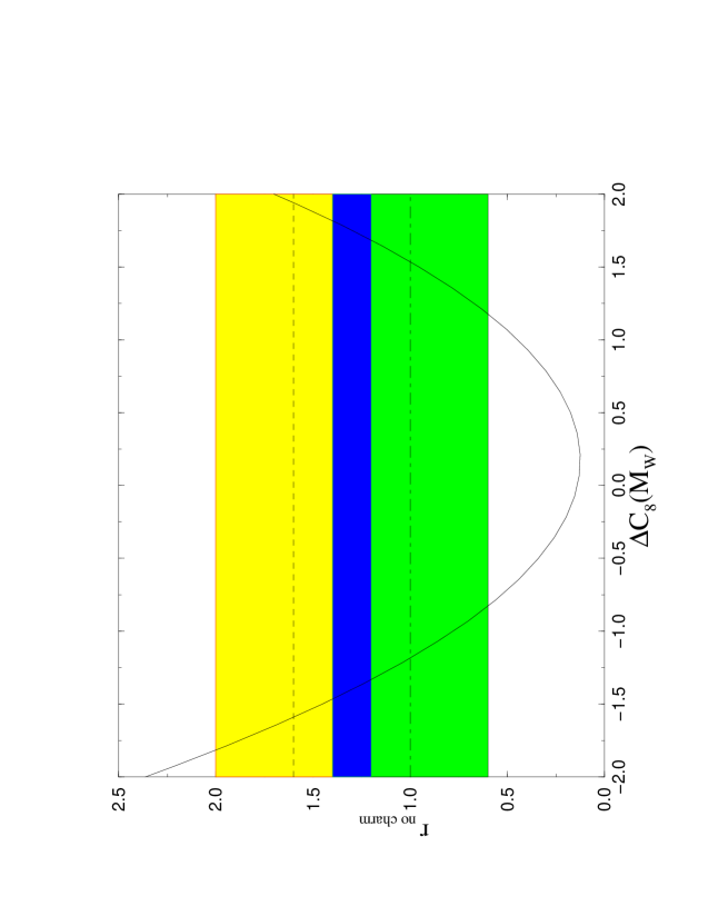
Figure 7: $r_{c/}$ vs. $\Delta C_{8}(M_{W})$ parameterizing new physics contributions to $C_{8}(M_{W})$. The dark shading marks the region $r_{c/}=1.0\pm 0.4$ needed to reproduce the experimental result for $n_{c}$ in (1). The lightly shaded area corresponds to $r_{c/}=1.6\pm 0.4$ obtained from the analysis in [14].

 

If one enlarges $C_{8}(M_{W})$ by a factor of 10 while keeping $C_{1-6}(M_{W})$ fixed, $r_{c/}$ grows by a factor of 5.5. The sensitivity of $r_{c/}$ to $C_{3-6}(M_{W})$ is much smaller, increasing the latter by a factor of 10 enhances $r_{c/}$ only by a factor of 1.6. Hence in the following we will only focus on $C_{8}\left(M_{W}\right)=-0.1+\Delta C_{8}(M_{W})$, where $\Delta C_{8}(M_{W})$ is the new physics contribution. For simplicity we will further assume that the CKM structure of the new contributions is the same as in the Standard model and neglect the possibility of new CP-violating phases by assuming $\Delta C_{8}(M_{W})$ to be real.

In Fig. 7 $r_{c/}$ is plotted versus $\Delta C_{8}(M_{W})$. Solving for $r_{c/}=1.0\pm 0.4$ yields two solutions:

$$\Delta C_{8}(M_{W})\;=\;-1.2\begin{array}[c]{l}\scriptstyle-0.3\\[-5.69054pt] \scriptstyle+0.4\end{array}\,,\qquad \qquad\Delta C_{8}(M_{W})\;=\;1.5\pm 0.3\,.$$ (50)

The central values correspond to an enhancement of the Standard Model value for $C_{8}(M_{W})$ by factors of 13 and $(-14)$. We hope to resolve the twofold ambiguity after calculating the contribution of $Q_{8}$ to $\Gamma(\overline{B}\rightarrow X_{c\overline{c}s})$.

The LEP data in (5) correspond to $r_{c/}=0.4\pm 0.5$ and

$$\Delta C_{8}(M_{W})\;=\;-0.5\begin{array}[c]{l}\scriptstyle-0.6\\[-5.69054pt] \scriptstyle+0.5\end{array}\,,\qquad \qquad\Delta C_{8}(M_{W})\;=\;0.9\begin{array}[c]{l}\scriptstyle+0.6\\[-5.69054pt] \scriptstyle-0.9\end{array}$$ (55)

showing the consistency of (5) with the Standard Model.

5 Conclusions

We have calculated two new contributions to the inclusive decay rates of B-mesons into various charmless final states: First we have obtained the results of penguin diagrams involving the operator $Q_{2}$ and a $c$- or $u$-quark in the loop putting special care on the renormalization scheme independence of our results. Second we have calculated the influence of the chromomagnetic dipole operator $Q_{8}$ on these decays. The former contributions have been found to dominate the branching fractions for $\overline{B}\rightarrow X_{u\overline{u}s}$, $\overline{B}\rightarrow X_{d\overline{d}s}$, $\overline{B}\rightarrow X_{s\overline{s}s}$, $\overline{B}\rightarrow X_{s\overline{s}d}$ and $\overline{B}\rightarrow X_{d\overline{d}d}$. The effect of $Q_{8}$ on these decay modes is also sizeable and decreases the rates. On the other hand the decay rate for $\overline{B}\rightarrow X_{u\overline{u}d}$ is only affected by a few percent. Our results increase the theoretical prediction for $Br(B\rightarrow\textit{no charm})$ by 36 %, which is not sufficient to explain the charm deficit observed in B-decays by ARGUS and CLEO. If a breakdown of quark-hadron duality due to intermediate $(c,\overline{c})$ resonances is to explain the “missing charm puzzle”, the phase space integrated penguin diagram with an internal $c$-quark must be larger than the perturbative result in the NDR scheme by roughly a factor of 9.

We have then analyzed the hypothesis that new physics effects enhance the coefficient $C_{8}$ of $Q_{8}$ and have performed a model independent fit of $C_{8}$ to the experimental data on $n_{c}$. The renormalization group evolution from $\mu=M_{W}$ to $\mu=m_{b}$ has been properly taken into account. One finds two solutions for $C_{8}$: For the central values of the theoretical input and the data of the $\Upsilon(4S)$ experiments $C_{8}(M_{W})$ must be larger by a factor of 13 or $(-14)$ than in the Standard Model, if the new physics contributions have the same CKM structure as the Standard Model penguin diagram.

Appendix A Scheme independence

Now we discuss the cancellation of scheme dependent terms between the NLO Wilson coefficients and the loop diagrams contained in $\Delta\Gamma_{cc}$ and $\Delta\Gamma_{peng}$. We define scheme independent combinations $\Delta\overline{\Gamma}_{cc}$, $\Delta\overline{\Gamma}_{peng}$ and $\Delta\overline{\Gamma}_{W}$, which allow a meaningful discussion of the numerical sizes of these separate contributions to $\Gamma$ as performed in sect. 4. Finally we comment on the scheme independence of $\Delta\Gamma_{8}$.

The NLO correction to the Wilson coefficients in (18) can be split into two parts:

$$\Delta C_{j}(\mu) = \sum_{k=1}^{6}J_{jk}C_{k}^{(0)}(\mu)+\Delta\overline{C}_{j}(\mu),\qquad\qquad j=1,\ldots 6.$$ (56)

$\Delta\overline{C}_{j}(\mu)$ contains the contributions stemming from the weak scale. It is independent of the renormalization scheme and proportional to $\alpha_{s}(M_{W})/\alpha_{s}(\mu)$. Yet the $J_{jk}$’s in (56) are scheme dependent. The precise definitions of the terms in (56) can be found in [28, 30]. We now absorb the terms involving $J_{jk}$ into $\Delta\overline{\Gamma}_{\mathit{cc}}$ and $\Delta\overline{\Gamma}_{\mathit{peng}}$, so that the latter become scheme independent.

The identification of scheme independent combinations of one-loop matrix elements and $J_{jk}$’s is most easily done, if one expresses the loop diagrams in terms of the tree-level matrix elements. The combination

$$r^{q^{\prime}}_{jk}\left(p^{2},m_{q^{\prime}},\mu\right) + J_{kj},\qquad\qquad\mbox{$j\leq 2$ and $k\geq 3$,}$$ (57)

of the coefficients in (16) and the $J_{kj}$’s is scheme independent [28]. Substituting $r^{q^{\prime}}_{jk}$ with (57) in (38) one finds the scheme independent quantity:

$$\Delta\overline{\Gamma}_{\mathit{peng}} = \Delta\Gamma_{\mathit{peng}}+\frac{G_{F}^{2}m_{b}^{5}}{64\pi^{3}}\,2\,{\rm Re}\,\left[-\,t\,\xi_{u}\xi_{t}^{*}\sum_{\scriptstyle i,j=1,2\atop\scriptstyle k=3,\dots 6}C_{i}^{(0)}C_{j}^{(0)}\,J_{ki}b_{jk}\right.$$ (58)

$$\phantom{\Delta\Gamma_{\mathit{peng}}+\frac{G_{F}^{2}m_{b}^{5}}{64\pi^{3}}\,2\,{\rm Re}\,\xi_{t}^{*}[}\;\left.+\left|\xi_{t}\right|^{2}\!\sum_{\scriptstyle i=1,2\atop\scriptstyle j,k=3,\ldots 6}\!C_{i}^{(0)}C_{j}^{(0)}J_{ki}b_{jk}\right].$$

Here $\xi_{t}^{*}=-\xi_{u}^{*}-\xi_{c}^{*}$ has been used. In the NDR scheme the $J_{ki}$’s in (58) evaluate to [28]

$$J_{31}=-0.877, \quad J_{32}^{\mathit{NDR}}=-0.532,$$

$$J_{41}=0.324, \quad J_{42}^{\mathit{NDR}}=-0.202,$$

$$J_{51}=0.557, \quad J_{52}^{\mathit{NDR}}=0.511,$$

$$J_{61}=0.146, \quad J_{62}^{\mathit{NDR}}=-0.677\,.$$ (59)

The $J_{k1}$’s in the first row of (59) do not depend on the renormalization scheme, because $r^{q^{\prime}}_{1j}=0$ in all schemes due to a vanishing colour factor.

In the same way one finds

$$\Delta\overline{\Gamma}_{cc} = t\,\frac{G_{F}^{2}m_{b}^{5}}{64\pi^{3}}\,2\,\left|\xi_{u}\right|^{2}\sum_{i,j=1}^{2}C_{i}^{(0)}C_{j}^{(0)}\left[h_{ij}+\sum_{k=1}^{2}J_{ki}b_{kj}\right].$$ (60)

Here the scheme dependence of the $h_{ij}$’s in (28) cancels with the one of the $J_{ki}$’s [28]:

$$J_{11}^{\mathit{NDR}}=J_{22}^{\mathit{NDR}}=\frac{631}{6348}=0.099, \qquad J_{12}^{\mathit{NDR}}=J_{21}^{\mathit{NDR}}=\frac{3233}{2116}=1.528.$$ (61)

If one inserts (56) into $\Delta\Gamma_{W}$, one finds the $J_{jk}$’s with $k\leq 2$ to appear exactly in the combinations entering (58) and (60). The remaining $J_{jk}$’s with $k\geq 3$ describing penguin-penguin mixing would cancel the scheme dependence of the loop diagrams of Fig. 3 and Fig. 3 with insertions of penguin operators $Q_{j}$, $j=3,\ldots 6$. Since the latter are omitted in our calculation, we must also leave out the $J_{jk}$’s with $k\geq 3$ in (56). This has been done in Tab. 1. $\Delta\overline{C}_{j}$ has been tabulated in the last line of Tab. 1 for illustration. It can be obtained from the other entries of the table with the help of (56), (61) and (59).

Finally $\Delta\overline{\Gamma}_{W}$ is simply obtained from $\Delta\Gamma_{W}$ in (26) by replacing $\Delta C_{j}$ with $\Delta\overline{C}_{j}$.

Unlike $C_{j}^{(0)}$, $j\leq 6$, $C_{8}^{(0)}$ is a two-loop quantity and therefore a priori scheme dependent. We understand $H$ in (12) to be renormalized such that the matrix elements $\langle\,dg\,|Q_{j}|\,b\,\rangle$ vanish at the one-loop level for $j=1,\ldots 6$. This ensures that $\Delta\Gamma_{8}$ as defined in (31) is scheme independent [27]. The thereby renormalized LO coefficient $C_{8}^{(0)}$ ist usually called $\widetilde{C}_{8}$ or $C_{8}^{(0),eff}$. In the NDR scheme this finite renormalization simply amounts to $C_{8}^{(0)}=C_{8}^{(0),NDR}+C_{5}^{(0)}$. Apart from $\Delta\Gamma_{8}$ this only affects the penguin diagram of $Q_{5}$ (cf. Fig. 3), which is a part of the neglected radiative corrections to penguin operators.

References

-
[1]
T.E. Browder, K. Honscheid and D. Pedrini,
hep-ph/9606354, to appear in
Annual Review of Nuclear and Particle Science.
T.E. Browder, hep-ph/9611373, talk at the ICHEP conference 1996, Warsaw, to appear in the proceedings.
J.D. Richman, hep-ex/9701014, talk at the ICHEP conference, Warsaw, 1996. -
[2]
B. Barish et al. (CLEO), Phys. Rev. Lett.76 (1996) 1570.
H. Albrecht et al. (ARGUS), Phys. Lett. B318 (1993) 397. -
[3]
I.I. Bigi, N. Uraltsev, and A. Vainshtein, Phys. Lett. B 293,
430 (1992); Erratum ibid. 297, 477 (1993).
B. Blok and M. Shifman, Nucl. Phys. B399 (1993) 441; ibid. 399 (1993) 459. -
[4]
A. Manohar and M. Wise, Phys. Rev. D 49, (1994) 1310.
B. Blok, L. Koyrakh, M. Shifman and A.I. Vainshtein, Phys. Rev. D49 (1994), 3356; Erratum ibid. D50 (1994) 3572.
T. Mannel, Nucl. Phys. B413 (1994) 396.
I.I. Bigi, M.A. Shifman, N.G. Uraltsev, A.I. Vainshtein, Int. J. Mod. Phys. A9 (1994) 2467. -
[5]
I.I. Bigi, B. Blok, M. Shifman, N. Uraltsev and
A. Vainshtein, in B decays, ed. S. Stone,
2nd edition, World Scientific, Singapore,
1994, 132.
I.I. Bigi, hep-ph/9508408. - [6] M. Neubert and C. Sachrajda, hep-ph/9603202.
- [7] I.J. Kroll, hep-ex/9602005, proceedings of the 17th Int. Symp. on Lepton Photon Interactions, Beijing, P.R. China, 1995, 204.
- [8] E. Bagan, P. Ball, V.M. Braun and P. Gosdzinsky, Nucl. Phys. B432 (1994) 3.
- [9] E. Bagan, P. Ball, B. Fiol and P. Gosdzinsky, Phys. Lett. B351 (1995) 546.
- [10] E. Bagan, P. Ball, V.M. Braun and P. Gosdzinsky, Phys. Lett. B342 (1995) 362; Erratum ibid B374 (1996) 363.
- [11] G. Altarelli and S. Petrarca, Phys. Lett. B261 (1991) 303.
- [12] M. Neubert, hep-ph/9605256, to appear in the proceedings of the 10th Les Rencontres de Physique de la Vallee d’Aoste, La Thuile, 1996.
- [13] G. Buchalla, I. Dunietz and H. Yamamoto, Phys. Lett. B364 (1995) 188.
- [14] I. Dunietz, J. Incandela, F.D. Snider and H. Yamamoto, hep-ph/9612421.
-
[15]
ALEPH coll., EPS-404, contribution to the Int. Europhysics Conf. on High Energy Physics, Brussels, 1995.
P. Abreu et al. (DELPHI), Z. Phys. C66 (1995) 323.
M. Acciarri et al. (L3) Z. Phys. C71 (1996) 379.
R. Akers et al. (OPAL), Z. Phys. C60 (1993) 199. - [16] M. Neubert, hep-ph/9610385, to appear in the proceedings of the 20th John Hopkins Workshop on Current Problems in Particle Theory, Heidelberg, 1996.
-
[17]
S. Bertolini, F. Borzumati and A. Masiero, Nucl. Phys. B294 (1987)
321.
A.L. Kagan, Phys. Rev. D51 (1995) 6196.
M. Ciuchini, E. Gabrielli and G.F. Giudice, Phys. Lett. B388 (1996) 353.
A.L. Kagan and J. Rathsman, hep-ph/9701300. - [18] W.F. Palmer and B. Stech, Phys. Rev. D48 (1993) 4174.
- [19] R. Fleischer, Z. Phys. C 58 (1993) 483.
- [20] G. Altarelli, G. Curci, G. Martinelli and S. Petrarca, Nucl. Phys. B187 (1981) 461.
- [21] W. A. Bardeen, A. J. Buras, D. W. Duke and T. Muta, Phys. Rev. D18 (1978) 3998.
- [22] A.F. Falk, Z. Ligeti, M. Neubert and Y. Nir, Phys. Lett. B326 (1994) 145.
- [23] G. Buchalla, Nucl. Phys. B391 (1993) 501.
- [24] A. J. Buras and R. Fleischer, Phys. Lett. B341 (1995) 379.
- [25] M. Ciuchini, E. Franco, G. Martinelli and L. Silvestrini, hep-ph/9703353.
-
[26]
M.A. Shifman, A.I. Vainshtein and V.I. Zakharov, Phys. Rev. D18
(1978) 2583 ; Erratum ibid. D19 (1979) 2815.
B. Grinstein, R. Springer and M.B. Wise, Phys. Lett. B202 (1988) 138; Nucl. Phys. B339 (1990) 269. -
[27]
M. Ciuchini, E. Franco, G. Martinelli, L. Reina and
L. Silvestrini, Phys. Lett. B316 (1993) 127.
M. Ciuchini, E. Franco, L. Reina and L. Silvestrini, Nucl. Phys. B421 (1994) 41.
M. Ciuchini, E. Franco, G. Martinelli, L. Reina and L. Silvestrini, Phys. Lett. B334 (1994) 137. -
[28]
A. J. Buras, M. Jamin, M. E. Lautenbacher and
P. H. Weisz,
Nucl. Phys. B370 (1992) 69; Addendum ibid B375 (1992) 501.
A. J. Buras, M. Jamin, M. E. Lautenbacher and P. H. Weisz,
Nucl. Phys. B400 (1993) 37. - [29] S. Bethke, hep-ex/9609014, talk given at the International Euroconference on Quantum Chromodynamics (QCD 96), Montpellier, 1996.
-
[30]
S. Herrlich and U. Nierste, Nucl. Phys. B455 (1995) 39.
S. Herrlich and U. Nierste, Nucl. Phys. B476 (1996) 27. - [31] H. Simma, G. Eilam and D. Wyler, Nucl. Phys. B352 (1991) 367.
- [32] Y. Nir, Phys. Lett. B221 (1989) 184.
- [33] I. Bigi, M. Shifman and N. Uraltsev, hep-ph/9703290.
- [34] M. Artuso, Nucl. Instrum. Meth. A384 (1996) 39.
-
[35]
S. Herrlich and U. Nierste, Phys. Rev. D52 (1995) 6505.
U. Nierste, hep-ph/9609310, talk given at the Workshop on K physics, Orsay, May/June 1996.