QCD Phenomenology of Charm Production at HERA

Abstract

We compare different schemes for the treatment of heavy quark production in Deep-Inelastic Scattering (DIS). For fully-integrated quantities such as $F_{2}(x,Q^{2})$, we advocate the use of the General-Massive Variable-Flavor-Number (GM-VFN) scheme; we present some results showing the progress of a Next-to-Leading Order calculation in this scheme. For differential quantities, the Fixed-Flavor-Number (FFN) scheme provides a more appropriate starting point. We present a new calculation of the azimuthal distribution of charm quark production in DIS. All results have been obtained using a Monte Carlo program under development.

Introduction

The theoretical treatment of heavy quark production has undergone much re-examination recently. A basic question is whether, or not, the charm quark (or bottom quark) should be included in the initial state, with its own parton density function (PDF). Traditionally, there have been two approaches used, which we shall call the Fixed-Flavor-Number (FFN) scheme and the Zero-Mass Variable-Flavor-Number (ZM-VFN) scheme. In the FFN scheme one does not include charm as a parton in the nucleon. The charm quark only occurs in the final state, and its mass is treated exactly. This is the standard approach for calculations of specific heavy flavor production process, such as charm production in deep inelastic scattering smith and charm or bottom production in hadron-hadron colliders dawson . Alternatively, in the ZM-VFN scheme one does include a heavy quark PDF in the nucleon at scales above the quark mass, but the quark is treated as massless in both the initial and final states. This is the approach used in most other inclusive jet calculations and parton shower Monte Carlo simulations. It also corresponds to the treatment of the charm and bottom quark in most global analyses of the parton density functions, including DIS structure functions.

Given these two seemingly contradictory methods of calculating heavy quark production cross sections, one may wonder which is correct. The answer, of course, is that both are correct at some level. The real question is what is the best method for calculating the particular set of observables under consideration at the energy scale of the processes being studied. For example, near the charm production threshold in deep inelastic scattering, the various energy scales, $Q^{2}\sim m_{c}^{2}\sim W^{2}$, are roughly equal, so that we have essentially a one scale problem. Since the FFN scheme treats this scale exactly, including the kinematics of the charm quark mass, it should be expected to do well here. However, at higher $Q^{2}$ scales the effect of the $m_{c}$ can be neglected, except when it occurs in large logarithms $\log(Q^{2}/m_{c}^{2})$. These can be resummed by invoking a charm quark parton density function and evolving up to $Q^{2}$. Thus, at higher energies the ZM-VFN scheme will be more accurate. As a side remark, we also note that the ZM-VFN scheme is necessary if one is to consider the possibility of a nonperturbative charm quark contribution brodsky to the nucleon PDF beyond that which is generated dynamically by the splitting of gluons.

In general we want a scheme that does the best job at including the largest corrections from higher orders in perturbation theory. Since much of the data is in an intermediate range of $Q^{2}$, neither the FFN nor the ZM-VFN schemes are completely adequate. For this purpose a General-Massive Variable-Flavor-Number (GM-VFN) scheme was devised ACOT . (It is sometimes referred to as ACOT, for the originators.) In this scheme the charm quark PDF evolves with massless evolution, but the heavy quark mass is kept everywhere else in the matrix elements and phase space. The leading order process $\gamma^{*}c\rightarrow c$ from the ZM-VFN scheme and the leading order process $\gamma^{*}g\rightarrow c\bar{c}$ from the FFN scheme are both included in the new scheme. However, to keep from double-counting, we must also subtract a term which is the convolution of the $g\rightarrow q$ splitting function with the $\gamma^{*}q\rightarrow q$ process. This is shown diagrammatically in figure 1. Note that, although the subtraction term may appear ad hoc here, it is in fact just the massive equivalent to the Altarelli-Parisi subtraction of the $1/\epsilon$ pole at next-to-leading order (NLO) in the ZM-VFN scheme.

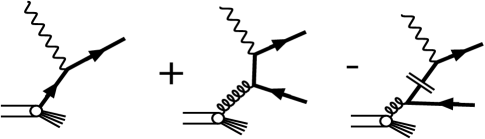
Figure 1: Feynman diagrams for LO GM-VFN scheme.

By including the three terms shown in figure 1 with massless evolution of the charm PDF, but full mass-dependence in the coefficient functions, we find that the calculation in the GM-VFN scheme agrees with the ZM-VFN scheme at large $Q^{2}$ and with the FFN scheme near threshold. The three terms in figure 1 constitute a Leading Order (LO) calculation if one considers the charm quark PDF to be $O(\alpha_{s})$. This makes sense in the absence of nonperturbative charm contributions since the charm quark PDF arises entirely from splitting of gluons and is consequently smaller than the gluon PDF. Furthermore, this method of $\alpha_{s}$ counting leads to reduced renormalization/factorization scale ($\mu$) dependence, as we shall see. This scheme also allows the inclusion of nonperturbative charm contributions to the nucleon PDF, which should exist at some level. A recently-proposed prescription by Martin et al. (MRRS) MRRS is similar in spirit to this. They use the conventional counting of $\alpha_{s}$ and split the heavy quark mass-dependence into a contribution to the splitting functions and a contribution to the coefficient functions. See the talk by Olness at this conference for a discussion of this issue olness .

For a more detailed discussion of the theory of heavy quark production, we refer to the talk by Tung at this conference tung . In the remainder of the present talk we describe the progress in implementing the GM-VFN scheme at next-to-leading order (NLO) in a Monte Carlo program. Currently, we have added the ${\cal O}(\alpha_{s})$ virtual and real ($\gamma^{*}c\rightarrow gc$) contributions to the charm excitation process, with the appropriate subtraction. This partial-NLO GM-VFN calculation incorporates all of the terms that are in the NLO calculation in the ZM-VFN scheme using the conventional $\alpha_{s}$-counting. The ${\cal O}(\alpha_{s})$ virtual and real corrections to the gluon- or light quark-initiated processes (and subtractions) that also contribute to the NLO GM-VFN scheme have not yet been included. However, we can still gain useful insight with the results so far.

Integrated observables – $F_{2}(x,Q^{2})$

As discussed above, the GM-VFN scheme should be the best method of calculating integrated observables, such as the charm contribution to $F_{2}(x,Q^{2})$. In figures 2a and 2b we compare the calculation of $F_{2}(x,Q^{2})$ in the various schemes. In figure 2a $F_{2}(x,Q^{2})$ is plotted as a function of $Q^{2}$ for $x=0.01$. We see that the NLO FFN calculation gives a sizeable increase over the LO FFN (tree-level gluon fusion) calculation, while the LO GM-VFN scheme is even higher. The partial-NLO GM-VFN, which should be most accurate at high $Q^{2}$, gives a small correction over LO GM-VFN. This indicates that the FFN tends to underestimate the cross section at high $Q^{2}$. At intermediate $Q^{2}$ we will need the full-NLO GM-VFN calculation, which is underway. Note that the GM-VFN scheme is much more economical than the the FFN scheme, since the largest contributions to the cross section are included at LO with substantially less work.

In figure 2b we show the $\mu$-dependence of $F_{2}(x,Q^{2})$ for $x=0.01$ and $Q=10$ GeV. In this plot the NLO FFN calculation only gives a slight improvement in the scale dependence over the LO FFN. However, the LO GM-VFN calculation is less sensitive to the choice of scale. The partial-NLO GM-VFN calculation actually has larger $\mu$-dependence than LO GM-VFN, but the remaining terms in the NLO GM-VFN calculation should improve this again. In both figures 2a and 2b the wiggles are just due to Monte Carlo statistics.

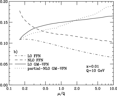
Figure 2: $F_{2}(x,Q^{2})$ in various schemes. a) versus $Q$ (GeV). b) versus $\mu/Q$. The NLO FFN curves are calculated using the code of Harris and Smith [6].

Differential observables – $\phi$ distribution

There are issues that make the GM-VFN scheme somewhat problematic when applied to differential distributions. The initial-state charm quark contributions include a resummation of collinear radiation diagrams, with the phase space of the anticharm quark always integrated out. Thus, the kinematics cannot be treated exactly. For instance, the transverse momentum distribution with respect to the $\gamma^{*}P$-axis is a delta-function, which can only make sense upon integration. In the FFN scheme, however, the $c\bar{c}+X$ final state is always treated exactly to a given order. Therefore, we expect that it should give a reasonable prediction for the differential distributions, as long as we are not too far from threshold.

In figure 4 we present a new plot, using our Monte Carlo in the FFN scheme at LO, of the distribution of the azimuthal angle $\phi$. This angle is defined as the angle between the lepton ($e\rightarrow e^{\prime}$) plane and the hadron ($c\bar{c}$) plane in a frame in which the $\gamma^{*}$ and the proton $P$ are collinear. By symmetry the distribution will be of the form $d\sigma/d\phi\sim A+B\cos{\phi}+C\cos{2\phi}$. In the plot we have made the cuts $0.01<y<0.7$, $10<Q^{2}<100$ GeV, and $p_{\perp}^{*}>2$ GeV, where $p_{\perp}^{*}$ is the transverse momentum with respect to the $\gamma^{*}P$-axis. We have also summed over the charm and anticharm contributions, which removes the $\cos{\phi}$ term. Although lab frame cuts will alter this distribution, they can easily be included in the Monte Carlo program.

Figure 3: Distribution in the azimuthal angle $\phi$.

We would like to thank Bryan Harris harris for providing us with the code to produce the NLO FFN plots.

References

- (1) Laenen, E., Riemersma, S., Smith, J., and van Neerven, W.L., Nucl. Phys. B392, 162 (1993).
- (2) Nason, P., Dawson, S., and Ellis, R.K., Nucl. Phys. B327, 607 (1988).
- (3) A model of this nonperturbative charm contribution to the nucleon PDF, called “intrinsic charm” is given by Brodsky, S., Peterson, C., and Sakai, N., Phys. Rev. D23, 2745 (1981).
- (4) Aivazis, M., Collins, J., Olness, I., and Tung, W., Phys. Rev. D50, 3102 (1994).
- (5) Martin, A., Roberts, R., Ryskin, M., and Stirling, W., preprint DTP/96/102, hep-ph/9612449 (1996).
- (6) Olness, F., these proceedings.
- (7) Tung, W., these proceedings.
- (8) Harris, B. and Smith, J., Nucl. Phys. B452, 109 (1995).