Structure Function Subgroup Summary

Abstract

We summarize the studies and discussions of the Structure Function subgroup of the QCD working group of the Snowmass 1996 Workshop: New Directions for High Energy Physics.

1 INTRODUCTION

Our knowledge of the structure functions of hadrons, and the parton density functions (PDFs) derived from them, has improved over time, due both to the steadily increasing quantity and precision of a wide variety of measurements, and a more sophisticated theoretical understanding of QCD. Structure functions, and PDFs, play a dual role: they are a necessary input to predictions for high momentum transfer processes involving hadrons, and they contain important information themselves about the underlying physics of hadrons. Their study is an essential element for future progress in the understanding of fundamental particles and interactions.

Because of the ubiquitousness of structure functions, the activities of the subgroup had significant and productive overlap with several other subgroups, and were focused in a number of different directions. This summary roughly follows these directions. We start with the precision of our knowledge of the PDFs. There was an attempt to define a ‘Snowmass convention’ on PDF errors, reviewing the experimental and theoretical input to the extraction of the PDFs and an appraisal of what is left to do. Next, we explore the important connection between the strong coupling constant, $\alpha_{s}$, and the structure functions. One of the important inputs provided by the structure functions is in the precise extraction of electroweak parameters at hadron colliders. The systematic uncertainties in the structure functions may be the limiting factor in the determination of electroweak parameters, and this is discussed in the subsequent section. There is then a review of some relevant aspects of heavy quark hadroproduction. Finally, as a summary, we present an $\{x,Q^{2}\}$ map of what is known and what is to come.

2 PRECISION OF PDFS AND GLOBAL ANALYSES

The extraction of PDFs from measurements is a complex process, involving information from different experiments and a range of phenomenological and theoretical input.

2.1 Experimental systematic errors

Since the extraction of the PDFs usually requires using data from different experiments, and since the most precise data are usually limited by systematic, rather than statistical, errors, it is important that the systematic errors are taken properly into account. In particular, it is necessary to understand the correlations of different systematic errors on the measurements within and across experiments. Several groups have begun to make this information available in electronic and tabular form. Contributions to these proceedings by Tim Bolton (NuTeV) and Allen Caldwell (ZEUS) give the details.

2.2 $\{x,Q^{2}\}$ Kinematic Map for PDFs

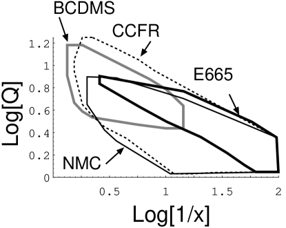
Figure 1: Fixed target DIS data. Note the full $\{x,Q^{2}\}$ region is clipped by the plot.

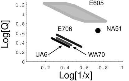
Figure 2: Drell-Yan (E605), Direct Photon (E706, WA70, UA6), and DY asymmetry (NA51) data.

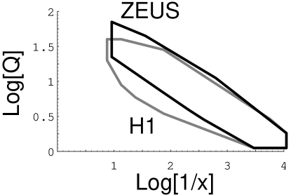
Figure 3: $ep$ collider data. Note the full $\{x,Q^{2}\}$ region is clipped by the plot.

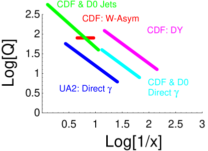
Figure 4: Hadron-hadron collider data.

Figure 5: Comparison of gluons obtained with pre-1995 DIS data (A-series) with those using current DIS data (B-series). (Cf., Ref. [1].)

Figure 6: Comparison of gluons obtained without jet data (C-series) with those obtained with jet data, D-series (CTEQ4Ax). (Cf., Ref. [1].)

Global QCD analysis of lepton-hadron and hadron-hadron processes has made steady progress in testing the consistency of perturbative QCD (pQCD) within many different sets of data, and in yielding increasingly detailed information on the universal parton distributions. We present a detailed compilation of the kinematic ranges covered by selected experiments from all high energy processes relevant for the determination of the universal parton distributions. This allows an overall view of the overlaps and the gaps in the systematic determination of parton distributions; hence, this compilation provides a useful guide to the planning of future experiments and to the design of strategies for global analyses.

These analyses incorporate diverse data sets including fixed-target deeply-inelastic scattering (DIS) data[2, 3] of BCDMS, CCFR, NMC, E665; collider DIS data of H1, ZEUS; lepton pair production (DY) data of E605, CDF; direct photon data of E706, WA70, UA6, CDF; DY asymmetry data of NA51; W-lepton asymmetry data of CDF; and hadronic inclusive jet data[4] of CDF and D0. The total number of data points from these experiments is $\sim 1300$, and these cover a wide region in the kinematic $\{x,Q^{2}\}$ space anchored by HERA data at small $x$ and Tevatron jet data at high $Q$.

We now present the various experimental processes. Note that while this is a comprehensive selection of experiments, it is by no means exhaustive; we have attempted to display those data which are characteristic for the structure function determination. In some cases, we have taken the liberty to interpret the data so as to facilitate comparison among the diverse processes we consider. Also note that we have not attempted to deal with the different precision of different measurements, or to separately consider the quark and gluon determination; the reader should keep these points in mind when comparing the figures.

The quark distributions inside the nucleon have been quite well determined from precise DIS and other processes, cf., Fig. 1:

$$\mu,\nu+N\rightarrow\mu,\nu+X\ .$$ (1)

Improved DIS data in the small-$x$ region is available from HERA, and this is of sufficient precision to be sensitive to the indirect influence of gluons via high order processes.

The Drell-Yan process is related by crossing to DIS. In lowest order QCD it is described by quark-antiquark annihilation:

$$q+\bar{q}\rightarrow\gamma^{*}\rightarrow\ell^{+}+\ell^{-}\ .$$ (2)

The kinematic coverage is shown in Fig. 2 and Fig. 4.

Recent emphasis has focused on the more elusive gluon distribution, $G(x,Q)$, which is strongly coupled to the measurement of $\alpha_{s}$. Direct photon production,

$$g+q\rightarrow\gamma+q\qquad,\qquad q+\bar{q}\rightarrow\gamma+g\quad,$$ (3)

in particular from the high statistics fixed target experiments, has long been regarded as the most useful source of information on $G(x,Q)$, cf., Fig. 2. However, there are a number of large theoretical uncertainties (e.g., significant scale dependence, and $k_{T}$ broadening of initial state partons due to gluon radiation)[5, 7] that need to be brought under control before direct photon data can place a tight constraint on the gluon distribution.

For example, the $k_{T}$ broadening due to soft gluon radiation is essentially a higher twist effect (but with a large coefficient), and should affect all hard scattering cross sections. The magnitude of the correction to the cross section should be on the order of $n(n+1)\langle k_{T}\rangle^{2}/(4p_{T}^{2})$, where $\langle k_{T}\rangle$ is the average $k_{T}$ in the hard scatter, and $n$ is the exponent of the differential cross section with respect to $p_{T}:$ ($d\sigma/dp_{T}\propto 1/p_{T}^{n}$). For the Tevatron collider regime, the effect should fall off as $\sim 1/p_{T}^{2}$, as is observed for example in direct photon production in CDF. For $p_{T}>50\,GeV$, the effect is negligible. For fixed target experiments, the effective value of $n$ is large and changes rapidly with $p_{T}$ (due to the rapidly falling parton distributions). The soft gluon radiation tends to make the cross section steeper at low $p_{T}$ and at high $p_{T}$, and to cause an overall normalization shift of a factor of 2.[5] There are several approximate methods to predict the effects of soft gluon radiation, as for example in gaussian $k_{T}$ smearing, or the incorporation of parton showers into a NLO Monte Carlo. Further understanding may await the development of a more formal treatment of the effect. Several theoretical ideas are under development.

Inclusive jet production in hadron-hadron collisions,

$$\{gg,\ q\bar{q}\}\rightarrow\{gg,\ q\bar{q}\}\quad,\quad g+\{q,\ \bar{q}\}\rightarrow g+\{q,\ \bar{q}\}\ ,$$ (4)

is very sensitive to $\alpha_{s}$ and $G(x,Q)$, (Fig. 4). NLO inclusive jet cross sections yield relatively small $\mu$ scale dependence for moderate to large $E_{t}$ values.[6] High precision data on single jet production is now available over a wide range of energies, $15\,GeV<E_{t}<450\,GeV$.[4] For $E_{T}>50GeV$, both the theoretical and experimental systematic errors are felt to be under control. Thus, it is natural to incorporate inclusive jet data in a global QCD analysis.

In reviewing the figures we see the large kinematic range which is explored by these processes. It is a useful exercise to overlay the curves according to the separate determination of the valence-quarks, light-sea-quarks, heavy-quarks, and gluons. Although there is no room here for such a presentation, we leave this as an exercise to the interested reader. Obviously, when comparing such a wide range of processes, one must keep in mind considerations beyond just the kinematic ranges. For example, the DIS and Drell-Yan processes are useful in determining the quark distributions, whereas the direct photon and photoproduction experiments yield information about the gluon distributions–though not with comparable accuracy; the determination of the gluon distribution is subject to many more theoretical and experimental uncertainties.

Likewise, the systematics for hadron-hadron and lepton-hadron processes are quite different. Specifically, while the hadron-hadron colliders can in principle determine parton distributions out to large $Q^{2}$, extractions of PDFs from these data are only beginning. DIS experiments probe small $x$ (HERA) and high $x$ (NuTeV), and low-mass Drell-Yan collider measurements yield complementary results at higher $Q^{2}$. This combination of experiments improves the reliability of the PDFs, allows for cross checks among the different experiments, and yields precise tests of the QCD evolution of the parton distributions.

2.2.1 Progress of PDFs

As new global PDF fits are being updated and improved, it can be difficult to quantify our progress as to how precisely we are measuring the hadronic structure. To illustrate this progress we consider sets of global PDF fits using various subsets of the complete data set.

First, we compare the A- and B-series of fits shown in Fig. 5. The A-series shows a selection of gluon PDFs extracted from pre-1995 DIS data using various values of $\alpha_{s}(M_{Z}^{2})$ as indicated in the figure. The B-series shows the same selection, but including the recent DIS data. By comparing the A- and B-series of fits, we found that recent DIS data [3] of NMC, E665, H1 and ZEUS considerably narrow down the allowed range of the parton distributions.

Next, we compare the B- and C-series of fits shown in Fig. 5 and Fig. 6. These fits were performed with the same data set, but the C-series fit used a more generalized parametrization with additional degrees of freedom. By contrasting the B- and C-series we see that we must be careful to ensure that our parameterization of the initial PDFs at $Q_{0}$ is not restricting the extracted distributions.

Finally, we compare the C- and D-series (CTEQ4Ax) of fits shown in Fig. 6. For the D-series fits, the Tevatron jet data was used, whereas this was excluded from the C-series fits. The jet data has a significant effect in more fully constraining $G(x,Q)$ as compared to the C-series. The quality of the final D-series fits (CTEQ4Ax) is indicative of the progress that has been made in this latest round of global analysis.

2.3 High $E_{t}$ Jets and Parton Distributions

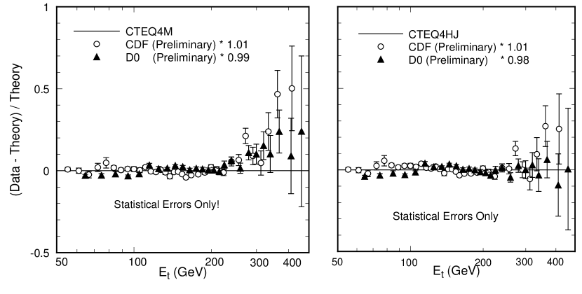
Figure 7: CDF and D0 data compared to NLO QCD using a) CTEQ4M and b) CTEQ4HJ. Cf., Refs. [7, 12, 13, 14].

Figure 8: (a) The CTEQ4HJ gluon distributions are compared to that of CTEQ3M: (b) the ratio of the CTEQ4HJ gluons to CTEQ3M. Cf., Ref. [7].

Table 1: Total $\chi^{2}$ ($\chi^{2}/point$) values and their distribution among the DIS and DY experiments for CTEQ4M and CTEQ4HJ. Cf., Ref. [1].

Experiment	#pts	CTEQ4M	CTEQ4HJ
DIS-Fixed Target	817	855.2(1.05)	884.3(1.08)
DIS-HERA	351	362.3(1.03)	352.9(1.01)
DY rel.	129	102.6(0.80)	105.5(0.82)
Total	1297	1320	1343

High statistics inclusive jet production measurements at the Tevatron have received much attention recently because the high jet $E_{t}$ cross-section[12, 13, 14] is larger than expected from NLO QCD calculations.[6] A comparison of the inclusive jet data of CDF and D0 and results is given in Fig. 7a. We see that there is a discernible rise of the data above the fit curve (horizontal axis) in the high $E_{t}$ region. The essential question is whether the high $E_{t}$ jet data can be explained in the conventional theoretical framework, or require the presence of “new physics”.[15, 8, 7]

Although inclusive jet data was included in the global fit of the PDF, it is understandable why the new parton distributions (e.g., CTEQ4M) still underestimate the experimental cross-section: these data points have large errors, so they do not carry much statistical weight in the fitting process, and the simple (unsigned) total $\chi^{2}$ is not sensitive to the pattern that the points are uniformly higher in the large $E_{t}$ region. A recent study investigated the feasibility of accommodating these data in the conventional QCD framework by exploiting the flexibility of $G(x,Q)$ at higher values of $x$ (where there are few independent constraints), while maintaining good agreement with other data sets in the global analysis.[7]

A result of this study is the CTEQ4HJ parton sets which are tailored to accommodate the high $E_{t}$ ($>200$ GeV) jets, as well as the other data of the global fit.[7] Fig. 7b compares predictions of CTEQ4HJ with the results of both CDF and D0. Results shown in Fig. 8 and Table 1 quantifies the changes in $\chi^{2}$ values due to the requirement of fitting the high $E_{t}$ jets. Compared to the best fit CTEQ4M, the overall $\chi^{2}$ for CTEQ4HJ is indeed only slightly higher.[9, 1] Thus the price for accommodating the high $E_{t}$ jets is negligible.

The much discussed high $E_{t}$ inclusive jet cross-section has been shown to be compatible with all existing data within the framework of conventional pQCD provided flexibility is given to the non-perturbative gluon distribution shape in the large-$x$ region.

Presently, we note that the direct photon data from the Fermilab experiment E706 are sensitive to the same $x$ range that affect the Tevatron high $E_{t}$ jet data. A more quantitative theoretical treatment of soft gluons may allow the direct photon data to probe this question more precisely. We will need such accurate, independent measurements of the large-$x$ gluons to verify if the high-$E_{t}$ jet puzzle is resolved, or whether we have only absorbed the “new physics” into the PDFs.

Nevertheless, this episode provides an instructive lesson: the precision with which we know the PDFs is not indicated from a simple comparison of different global fit sets. These fits proceed from similar assumptions and procedures, so their relative agreement should not be taken as assurance of our knowledge of the PDFs. In the present case, the gluon density was naively estimated to be less than 10-20% (in the $x$ kinematic range relevant for high $E_{t}$ jet production) from a simple comparison of different PDF sets. Surprisingly, a large change was eventually required (and accommodated) by the data (assuming the Tevatron result is not an indication of some new physics).

2.4 Challenges for Global Fitting

Global fitting of PDFs is a highly complex procedure which is both an art and a science. This requires fitting a large number of data points from diverse experiments with differing systematics. Furthermore, the data are compared with NLO theory which introduces additional complications on the theoretical side.

There was extensive discussion as to how to determine the uncertainty of the PDFs. We note that one of the most important uncertainties for the PDFs is the choice of $\alpha_{S}$, since this affects the gluon distribution directly as well as the singlet quarks. Both MRS and CTEQ now provide different PDFs with different choices of $\alpha_{S}$, this is a big improvement in determining the uncertainty of PDFs. But this group did not succeed in answering all the questions related to the goal of a true one-standard-deviation covariance matrix of PDF uncertainties, although we did focus on some points that deserve further study. We list some of these below.

1. A reminder: when adding two experiments, you simply add their $\chi^{2}$’s, and $\Delta\chi^{2}=1$ of the total $\chi^{2}$ is one $\sigma$.

   1. Due to direct photon theory $\mu$-scale and $k_{T}$ uncertainties, there is no way to define one standard deviation for these data. The handling of the $\mu$-scale is done differently in different groups and can lead to somewhat different gluon distributions.

   2. Other “choices” can lead to significant differences in $\chi^{2}$ ($\Delta\chi^{2}\approx 50-100$ units is typical). These choices include which data sets to use, the starting $Q_{0}$ value, etc. One example is the small-x CCFR neutrino data which disagrees with the electron/muon DIS data. This difference is unlikely to be caused entirely by parton distributions, and how this is handled in the global fits can cause significant changes in the global $\chi^{2}$.

2. Many experiments do not provide correlation matrices, and we’ve never seen a correlation matrix for a theoretical uncertainty. Without both of these for every experiment, one cannot expect $\Delta\chi^{2}=1$ to work.

3. In principle we should add in LEP/tau/lattice constraints on $\alpha_{S}$. But if they are treated as only a single data point, they will be swamped by the other 1200 points. (This would not be true if $\Delta\chi^{2}=1$ were valid.)

4. What to do about the charm mass in DIS? It will change $F_{2}$ predictions, but the resulting parton distributions then have a different definition of “heavy quark in the proton” and this must be accounted for in the theoretical calculations.

5. When the CDF W asymmetry and NA51 data were added (the change between CTEQ2 and CTEQ3), they gave a consistent picture of $\bar{u}$ and $\bar{d}$. But the $\chi^{2}$ went up for the rest of the experiments by 30! Once again $\Delta\chi^{2}=1$ is invalid. The choice was to accept the larger $\chi^{2}$’s to incorporate the new data presented.

6. What about higher twists? Should a higher twist theoretical uncertainty be added to DIS data?

2.5 Choice of Parametrization

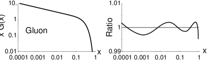
Figure 9: a) The gluon distribution $xG(x)$ at $Q_{0}=1.6GeV$ using the MRS and CTEQ parametrizations. The two curves are indistinguishable in this plot. b) Fractional deviation for gluon of the CTEQ and MRS parametrizations. Note the full range of the y-axis is $\pm 1\%$.

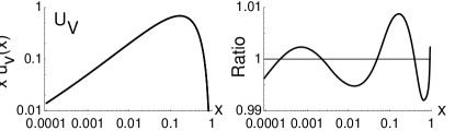
Figure 10: a) The u-valence distribution $xu_{v}(x)$ at $Q_{0}=1.6GeV$ using the MRS and CTEQ parametrizations. The two curves are indistinguishable in this plot. b) Fractional deviation for u-valence of the CTEQ and MRS parametrizations. Note the full range of the y-axis is $\pm 1\%$.

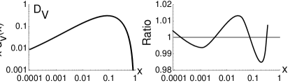
Figure 11: a) The d-valence distribution $xd_{v}(x)$ at $Q_{0}=1.6GeV$ using the MRS and CTEQ parametrizations. The two curves are indistinguishable in this plot. b) Fractional deviation for d-valence of the CTEQ and MRS parametrizations. Note the full range of the y-axis is $\pm 2\%$.

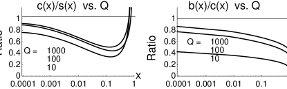
Figure 12: The ratio of a) $c(x)/s(x)$ and b) $b(x)/c(x)$ for a range of $Q$. For increasing $Q$, the evolution reduces any difference between the distributions.

The choice of boundary conditions for the PDFs at the initial $Q_{0}$ has received increasing attention as the accuracy of data improves.[1, 8, 9, 10] Although the DGLAP evolution equation clearly tells us how to relate PDFs at differing scales, the form of the distribution at $Q_{0}$ cannot yet be derived from first principles, and must be extracted from data. For this purpose, it is practical to choose a parametrization for the PDFs at the initial $Q_{0}$ with a small number of free parameters that can be fit to the data.

A question that was repeatedly raised in the workshop is the extent to which the choice of parametrization limits the extracted PDFs of the global fit. It is important to note that the evolution equation for the global fits is solved numerically on an $\{x,Q^{2}\}$ grid. Therefore the issue of the parametrization is only relevant at $Q_{0}$. For $Q>Q_{0}$, the parametrized form is replaced by a discrete $\{x,Q^{2}\}$ grid.

To approach these questions in a quantitative manner, we performed a simple exercise to examine the potential difference of PDFs that can be attributed to different choices of parametrizations. Specifically, we investigated the difference between the MRS[8] and CTEQ[9] parametrizations, which take the general form:

MRS:

$$f(x,Q)=a_{0}x^{a_{1}}(1-x)^{a_{2}}(1+a_{3}\sqrt{x}+a_{4}x)$$ (5)

CTEQ:

$$f(x,Q)=b_{0}x^{b_{1}}(1-x)^{b_{2}}(1+b_{3}x^{b_{4}})$$ (6)

We used the CTEQ3M PDF set at $Q_{0}=1.6\,GeV$ (which is naturally described by the CTEQ parametrization shown above), and performed a fit to describe the same PDF set using the MRS parametrization. Note that this is an academic exercise that does not fit data, but rather explores the flexibility of the parametrizations.

If we can accurately describe the CTEQ3 PDFs with the MRS form, then it is plausible that the particular parametrization choice for the PDFs has little consequence. However, if we cannot accurately describe the CTEQ3 PDFs with the MRS form, we will need to investigate more thoroughly whether the parametrization introduces a strong bias as to the possible PDFs which will come from the global fitting procedure.

In Figs. 9, 10, and 11, we plot both the CTEQ3 PDFs and the fit to the CTEQ3 PDFs using the MRS parametrized form, Eq. 5. We only show the gluon, u-valence, and d-valence; the results for the sea-quarks will be similar to the gluon. First we plot $x\,f(x)$ at $Q_{0}=1.6\,GeV$ on a Log-Log scale. The two separate curves are indistinguishable in this plot. To better illustrate the differences, we plot the fractional difference between the two PDFs. Observing that the scale on this plot is $\leq 2\%$, we see that the variation over the range $x=[10^{-4},1]$ is relatively small. We find larger deviations in the high $x$ region, but the significance of this is diminished by the fact that the PDFs are small in this region.

Although we do not claim that this is an exhaustive investigation, this simple exercise appears to indicate that the PDFs extracted from a global fit should be insensitive to the choice of the above parametrizations (Eq. 5). One might speculate that the same conclusion would also hold for other parametrizations; however, such an exercise has yet to be performed.

Furthermore, since the QCD evolution is stable as one evolves up to higher values of $Q$, any small differences at $Q_{0}$ will decrease for $Q>Q_{0}$. We can roughly see this effect by examing the ratios of $c(x)/s(x)$ and $b(x)/c(x)$ as shown in Fig. 12. For example, at $Q=10\,GeV$, the b-quark is less than half of the c-quark distribution; at $Q=100\,GeV$ the b-quark distribution is significantly closer to the c-quark.[11] This observation suggests that the small differences we observed at $Q_{0}=1.6\,GeV$ will quickly wash out as we evolve upwards.

The above observations, however, only apply in regions of $x$ where PDFs are well-determined; and they cannot be taken literally without qualification. An important example which illustrates the importance of exercising caution is the behavior of the gluon distribution at large $x$ brought to focus by the high $E_{t}$ jet data, as discussed in the last section. Whereas, using “conventional” parametrization of the form Eq.(5), GMRS [8] found it impossible to fit the jet results along with the rest of the global data, CTEQ showed that allowing for a more flexible parametrization of the gluon distribution at large $x$ can accommodate both. To accomplish this, one will need a functional form such as Eq.(6), with $b_{4}$ substantially bigger than 1, or equivalently, $e^{b_{4}x}$ in place of $x^{b_{4}}$. (Since $0<x<1$, and the whole expression is multiplied by $(1-x)^{b_{2}}$ which is steeply falling, $G(x,Q)$ is still well-behaved.) The difference in the size of $G(x,Q)$ resulting from these parametrizations can be as much as 100% at $x=0.5$, as shown in Fig. 8.

3 STRUCTURE FUNCTIONS AND $\alpha_{S}$

Structure functions are important in that they give us information on the value of $\alpha_{s}$, and also in that they are often inputs to many different measurements, some of which themselves are used to determine $\alpha_{s}$. In this summary of the work of the joint $\alpha_{s}$-structure function groups we investigate how structure functions themselves give us direct information on $\alpha_{s}$, and the expected uncertainties of possible new measurements of structure functions at future proposed machines. There are two categories of structure function analyses which result in an $\alpha_{s}$ measurement: $Q^{2}$ evolution of structure functions, and measurements of sum rules, which pertain to the integrals of specific structure functions over $x$. Since the theoretical and experimental errors are comparable for some of these analyses, this report examines how improvements might be made in both areas.

On the experimental side of the study, we consider a $\mu p$ collider or an $ep$ collider, and also a neutrino scattering experiment at a $\mu^{+}\mu^{-}$ collider. Given the current level of error in $\alpha_{s}$ measurements, we consider here only analyses which may result in few per cent or less error on $\alpha_{s}(M_{Z}^{2})$. To address the theoretical issues within the scope of this report we can at best point out the largest problems and how they are currently being investigated, in hopes of inspiring theorists to devote more time to them.

3.1 Evolution of Structure Functions

When looking at the $Q^{2}$ evolution of structure functions, one can use the DGL-Altarelli-Parisi Equations to find $\alpha_{s}$ [16]. In the case of the non-singlet structure functions the evolution as a function of $Q^{2}$ is simply related to $\alpha_{s}$ and the non-singlet structure function itself. In the case of the singlet structure functions, the evolution is related to $\alpha_{s}$, the structure function itself, AND the gluon distribution, which complicates matters. In either case care must be taken avoid large higher twist effects, which are particularly important at low $Q^{2}$.

Non-singlet structure functions can be measured in both neutrino and charged lepton scattering experiments. One way is by taking the average of $xF_{3}^{\nu N}$ and $xF_{3}^{\overline{\nu}N}$, where $\nu N$ in the superscript indicates the presence of an isoscalar target. Similarly, averaging $xW_{3}^{l^{+}d}$ and $xW_{3}^{l^{-}d}$ also results in a pure non-singlet structure function, where the lepton is either an electron or muon, and the scattering center is a deuteron. Finally, one can use the structure function $F_{2}^{\nu N}$ or $F_{2}^{l^{\pm}N}$ at high x, since there are virtually no sea quarks at high $x$.

Many high statistics determinations of $\alpha_{s}$ have to date been performed, using a variety of techniques. By fitting only $xF_{3}$ or $F_{2}$ at high $x$, one can do a pure non-singlet fit to the evolution, with no dependences on the gluon distribution. Given the wealth of precise data in charged lepton scattering structure functions, however, there are also determinations of $\alpha_{s}$ from fitting $F_{2}$ at all $x$, but including a contribution to the evolution from the gluons. These two different kinds of determinations do not show any systematic difference in the final result, as is shown in table 2.

Table 2: A selection of $\alpha_{s}$ measurements from structure functions, and the total error on $\alpha_{s}(M_{Z}^{2})$.

Method	Experiment	$Q^{2}$	$\alpha_{s}$($M_{Z}^{2}$)
$xF_{3}$ only	CCFR [17]	25	$.118\pm.007$
$xF_{3}$ and $F_{2}$	CCFR [17]	25	$.119\pm.0055$
$F_{2}$ low $x$	NMC [18]	7	$.118\pm.015$
$F_{2}$ high $x$	SLAC$/$BCDMS [19]	50	$.113\pm.005$
$F_{2}$ low $x$	HERA [20]	4-100	$.120\pm.010$

The errors listed in 2 are deceiving, however, because in fact they are all dominated by either experimental or theoretical systematic errors. In the remainder of this section we consider the largest two systematic errors, and how new machines (and new calculations) could hopefully reduce these errors.

3.1.1 Experimental Errors on $\alpha_{s}$ and possible improvements

The dominant experimental systematic error in the measurements listed in the table come from energy uncertainties. These can come from spectrometer resolution, calibration uncertainty in the detector, or overall detector energy scale. The key to improving the overall experimental error in these measurements is not higher statistics or higher energies, but better calorimetry, and better calibration techniques. The challenge in determining the energy scale in deep inelastic scattering experiments is in finding some “standard candle” from which to calibrate. For example, if there were some way of measuring the known mass of some particle decaying in the system, or if the initial beam energy was very well known because of accelerator constraints, this could substantially improve the energy scale determination over previous experiments.

A number of machines have been proposed at this workshop in a variety of energies and initial particles. While it is true that machines (and experiments) are not proposed these days to do precise QCD measurements alone, there are some interesting possibilities that may arise from these machines.

Because of other considerations (namely the rise of $F_{2}$ at low $x$) a lepton/hadron collider is an attractive possibility. Currently, however, the HERA $\alpha_{s}$ experimental error is dominated by uncertainties in the $x$ distribution of the structure functions measured, (particularly that of the gluon). In order to do a DGLAP-style evolution measurement in a lepton hadron collider, one would need to have both $\ell^{+}p$ and $\ell^{-}p$ collisions, measure the different cross sections, and extract a non-singlet structure function. The statistics needed for a precise structure function measurement at the energies that have been proposed would be well above current HERA expectations, and the higher in $Q^{2}$ these machines operate the lower the cross section, and the smaller the effect one is trying to measure.

Another intriguing possibility would be a neutrino experiment at a muon collider. A 2TeV muon collider could (with considerable engineering) make very high rate 800GeV neutrino and antineutrino beams. If one knew the muon beam energy very well (taking as an example how well the LEP energy scale is now known after much work!) then a neutrino beam coming from muon decays would be at a very well-understood energy as well. There would be negligible production uncertainty from a neutrino beam coming from a muon beam, and the rates for such a beam would be astronomical simply starting with the current proposals for muon intensities in the accelerator.

3.1.2 Theoretical Errors on $\alpha_{s}$ and possible improvements

Currently the renormalization and factorization scale uncertainties dominate the theoretical error on $\alpha_{s}$ from structure function evolution. This is true for both singlet and non-singlet structure functions evolution. By assuming the factorization and renormalization scales were $k_{1}\mbox{$Q^{2}$}$ and $k_{2}\mbox{$Q^{2}$}$ respectively, and varying $k_{1}$ and $k_{2}$ between 0.10 and 4, Virchaux and Milsztajn arrive at an error of $\delta(\mbox{$\alpha_{s}$}(\mbox{$M_{Z}^{2}$}))=.004$.[19]. They claim that the overall $\chi^{2}$ of the fit did not increase significantly when these variations were made. Similar or larger QCD scale errors apply to the other $\alpha_{s}$ measurements listed in table 2. Certainly the most straightforward (and perhaps naive) way to reduce this error would be to calculate the next higher-order term in the DGLAP equations.

Still another method of reducing these errors is to actually fit for $k_{1}$ and $k_{2}$, and see what the resulting error on these values are within the fit. By floating those constants, however, one is assuming QCD works, and getting a good fit for one consistent value of $\Lambda_{\overline{MS}}$ in the experiment can no longer be claimed by itself as a test of QCD. If $k_{1}$ and $k_{2}$ are floated, one does not test QCD until one compares one experiment’s $\alpha_{s}$ value with another experiment’s value. Furthermore, if the fit prefers values of $k_{1}$ and $k_{2}$ far away from one, one would also question the validity of the measurement.

3.2 Sum Rules are Better than Others

The two sum rules that have thus far been used to measure $\alpha_{s}$ are the Gross Llewellyn Smith sum rule [21] and the Bjorken sum rule [22], which are related to $xF_{3}$, and the polarized structure functions $g_{n}(x)$ and $g_{p}(x)$ respectively. Since these methods of determining $\alpha_{s}$ are far less mature than the structure function analysis, the corresponding experimental errors on $\alpha_{s}$ are much larger. Since both Sum Rules come are fundamental theoretical predictions, and the higher order corrections to the sum rules are so straightforward to compute, the QCD scale error on these measurements is much smaller than those of the evolution measurements. Table 3 gives a list of systematic and statistical errors for both sum rules.

Table 3: Table of errors on $\alpha_{s}(M_{Z}^{2})$ from Sum Rules. ^† From E142 result, E154 claims should be higher

	$\delta\mbox{$\alpha_{s}$}(\mbox{$M_{Z}^{2}$})$
Error Source	GLS	Bjorken
Statistical	.004	$<.001$
Low $x$ extrapolation	.002	.005†
Overall Normalization	.003	.002
Experimental Systematics	.004	.006
Higher Twist	.005	.003-.008
QCD Scale Dependence	.001	.002

3.2.1 Low $x$ Uncertainties

The largest uncertainties in sum rule measurements come from the fact that they involve integrals from $x=0$ to $x=1$. Of course no experiment can measure all the way down to $x=0$, and the closer to 0 one can reach the smaller the error in extrapolating from the lowest data point to zero will be. What is usually done to extrapolate to $x=0$ is a functional form is assumed, and the data are either fit to that functional form and the resulting parameters are checked with a theory, or if the data do not have enough statistical precision some functional form is simply assumed. While for the GLS sum rule the data seem to agree with simple quark counting arguments for the form of $xF_{3}$ at low $x$, the newest data from SLAC E154 (shown after Snowmass’96 at ICHEP96) do not fit to a function whose integral converges as $x$ goes to 0. The collaboration does not yet report a measurement of $\alpha_{s}$ from their new data, saying that the low $x$ behavior of the integral is too uncertain; however, this analysis is in progress. For future improvement on the Bjorken Sum Rule one will need to go to lower $x$ than what has currently been reached ($x=.015$). If the Bjorken integral is not finite then much more is called into question than the validity of QCD!

Another uncertainty associated with the low $x$ region is that one also needs to go to low $Q^{2}$ to measure low $x$. At low $Q^{2}$ higher twist uncertainties become important, and these higher twist contributions have never been measured for these sum rules. The present state of higher twist calculations for DIS sum rules is given in reference [27], which discusses results from many models of higher twist calculations, including QCD Sum Rules, and a non-relativistic quark model. Again, there is more trouble associated with the Bjorken Sum Rule than the GLS sum rule, because the different models predict very different higher twist contributions to the former, while agreeing at the $50\%$ level for the latter. So, whether one takes as the higher twist error the spread of theoretical predictions or the error on one such prediction (shown in the table above) one can arrive at very different errors. In either case that error is significant at the currently relevant $Q^{2}$ region. Unless a proven agreed-upon method of higher twist calculations arises the best bet in the future will be to simply fit the sum rule results for a higher twist contribution and an $\alpha_{s}$ contribution. This will require much higher statistical precision in the structure function measurements themselves than what is currently available.

3.2.2 Normalization Uncertainties

Finally, if one proposes to improve these measurements by going to a higher $Q^{2}$  the next most important error (assuming one has solved the problem of extrapolating to low $x$) will be the overall normalization error. Since the effect one is measuring is proportional to 1-$\alpha_{s}$and not $\alpha_{s}$, as $Q^{2}$ gets larger and $\alpha_{s}$ gets smaller then an overall $1\%$ error on the normalization of the structure functions (and hence the integral itself) turns into a larger fractional error on $\alpha_{s}$. This is shown quantitatively in figure 13, which shows the effects of the higher twist error as a function of $Q^{2}$ and a $1\%$ normalization error on the structure functions as a function of $Q^{2}$. The sum of the two errors in quadrature show that measuring the sum rules at a $Q^{2}$ above 100 GeV² will not reduce the overall error for even an ambitious normalization error of $0.25\%$. The current normalization error on the overall $\nu$-nucleon cross section is $1\%$, and the error on the ratio of $\nu$ and ${\overline{\nu}}$ cross sections is another $1\%$, which translates into presently a total $xF_{3}$ normalization of $1.4\%$. There are currently no plans to improve this measurement, one would need a tagged neutrino beam (which might be possible with a muon beam at a muon collider) to do so.

Figure 13: Variation of (a) higher twist, (b) $1\%$ normalization errors, and (c) the sum in quadrature of the two as a function of $Q^{2}$ for the GLS sum rule.

3.3 $\alpha_{s}$ conclusions

Structure functions and QCD provide us with the possibility of two complementary measurements of $\alpha_{s}$; the $Q^{2}$ evolution and sum rules. The current errors on $\alpha_{s}$ from structure function evolution are in the $4-5\%$ range, and will be improved only with a reduction of the renormalization and factorization scale uncertainties. For this, next to next to leading order (NNLO) corrections to the DGLAP equations must be computed. By far the most important experimental uncertainty in evolution measurements comes from how precisely experiments know their energy scale and resolution. Sum Rules have very different outstanding issues, namely the low $x$ uncertainty and measurement, and also the higher twist terms. The best way to eliminate higher twist uncertainties would be to simply measure their contributions in the lowest $Q^{2}$  yet still have enough statistics at higher $Q^{2}$ for a measurement of $\alpha_{s}$. While the sum rule analyses would benefit from much higher statistics, in general, to arrive at new measurements of $\alpha_{s}$ from structure functions we must do more than simply raise the energies of the experiments and run them longer!

4 STRUCTURE FUNCTION INPUTS TO PRECISION ELECTROWEAK MEASUREMENTS

Structure functions are inputs to many precision electroweak measurements–a few examples are from $sin^{2}\theta_{W}$ measured in $\nu$N scattering and global electroweak fits which include $\alpha_{s}$ from structure function data along with other fundamental parameters. A measurement expected to have significant experimental improvement in the future such that the structure function uncertainty becomes important relative to other uncertainties is the W mass ($M_{W}$) measurement from on-shell production at collider experiments. Even at the current level of precision of this analysis there are outstanding questions about how that uncertainty is evaluated, and whether this could be improved, even before new experiments come around.

At a hadron collider experiment, the W mass itself cannot be directly measured on an event by event basis, because the clean signatures of $W$ production contain a charged lepton and therefore also contain a neutrino. Furthermore, the initial center of mass energy of the partons which interact to give a $W$ is not known, so one cannot simply require the total momenta to balance to give the energy of the outgoing neutrino. One can use the constraint that the total initial transverse momentum is zero, however. The way the mass is then measured in an experiment is that the transverse mass is computed, $M_{T}=\sqrt{2p_{t}^{\ell}p_{t}^{\nu}(1-\cos\phi^{\ell\nu})}$, where $p_{t}^{\ell,\nu}$ are the transverse momenta of the charged lepton and neutrino, and $\phi^{\ell\nu}$ is the angle between the charged lepton and neutrino in the transverse plane. The shape of the $M_{T}$ distribution is then extremely sensitive to $M_{W}$, but is also dependent on the parton distributions used in the Monte Carlo simulation, in particular, the transverse component of $u-d$.

Table 4 gives the uncertainty in $M_{W}$ from CDF and D0 from direct production, and measurement of the transverse mass [29].

Table 4: Table of uncertainties for both the CDF and D0 $W$ mass measurements, for different final states ($e\nu$ or $\mu\nu$) and different run periods (Ia,Ib).

Source	CDF		D0	D0
	Ia		Ia	Ib
	$e$	$\mu$	$e$	$e$
Statistics	145	205	140	70
Lepton Scale	120	50	160	80
Lepton Resolution	80	60	85	50
Lepton Efficiency	25	10	30	20
$P_{T}^{W}$, PDF	65	65	65	65
$P_{T}^{\rm\textstyle Recoil}$ Model	60	60	100	55
Underlying Event
in Lepton Towers	10	5	35	30
Background	10	25	35	15
Trigger Bias	0	25	-	-
QCD Higher Order Terms	20	20	-	-
QED Radiative Corrections	20	20	20	20
Luminosity Dependence	-	-	-	70
Total	180		270	170

Currently the structure function uncertainty is estimated by doing the analysis with several different sets of parton distribution functions, and comparing the results, using the W asymmetry measurement as another constraint. Figure 14 shows the measured W asymmetry from CDF and the predictions from various PDFs [30]. Given that most of these PDFs come from the same input data (deep inelastic structure functions), the spread of the predictions represents an error in the technique of parametrizing the distribution which accounts for the W asymmetry, not the error on the distribution itself. By requiring a PDF to reproduce the measured W asymmetry, one is choosing a more appropriate parametrization, but one must go further to assign errors on that specific parametrization.

Figure 14: The W asymmetry as measured in CDF and the prediction of various different parton distribution functions.

Figure 15 shows the resulting change in $M_{W}$ for different PDFs, and how many standard deviations each PDF is from predicting the $W$ asymmetry [28].

Figure 15: The change in W mass versus the signed standard deviation of agreement with the measured W charge asymmetry for different PDFs.

The problem with estimating this uncertainty by comparing different PDFs is the following: if all of these PDFs are simply different parametrizations which come from the same sets of deep inelastic scattering data, then two different PDFs do not necessarily encompass the uncertainty on whatever quark distributions are relevant. There must be errors on the PDFs in order for the correct error on the W mass uncertainty to be evaluated. Of course, since at the present time there are no errors given with PDFs, this is not possible.

There was much discussion at Snowmass about the difficulties associated with assigning errors to PDFs, and one should refer to that section of this write-up, and a separate submission by Tim Bolton on this topic. Given that the job of assigning those errors is one that is far from completion, a temporary solution was suggested at this meeting. Namely, a PDF-generator could produce a set of PDFs that span the range of the possible values of the distribution in question. For example, for the jet $E_{T}$ analysis, a set of PDFs with different values of $\alpha_{s}$ has been generated. Similarly, a set of PDFs with the acceptable range of $u-d$, which is important for the W mass measurement ( and also the W asymmetry measurement) could also be generated. Then the $M_{W}$ analysis could simply compare the different PDFs in one set provided for an estimate on the $M_{W}$ error from uncertainty in the PDFs, and compare different parametrizations for the uncertainty on the parametrization.

Furthermore, much care must taken when using the measured $W$ asymmetry to constrain the $W$ mass error from PDFs. Since the $W$ mass is measured using a distribution dependent mostly on transverse quantities, and the asymmetries depend on longitudinal differences between the $u$ and $d$ quark distributions, the correlations (and/or lack of correlations) must be taken into account appropriately.

In order to use PDFs to their full potential, and also make precision measurements at hadron collider experiments, collaboration between PDF-generators and experimenters is essential. The $W$ mass illustrates where this would be useful probably better than any other precision electroweak measurement. Given that the future seems to be evolving towards higher energy hadron colliders, the necessity of errors on parton distribution functions can only increase, as will the care required in using these functions correctly.

5 HEAVY QUARK HADROPRODUCTION

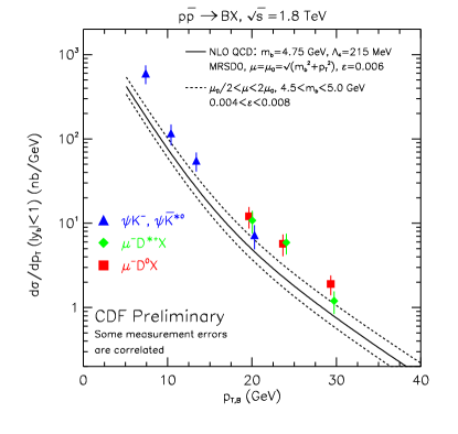
Figure 16: Heavy quark hadroproduction data. Cf., Ref. [31].

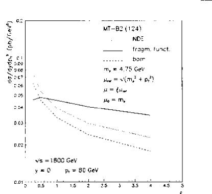
Figure 17: Scale dependence of the heavy quark hadroproduction cross section as a function of $\mu=\xi\mu_{ref}$ at $y=0$ and $p_{t}=80\,{\rm GeV}$. The NDE curve is the calculation of Ref. [32]. The fragm., funct. and born curves are the calculation of Ref. [34].

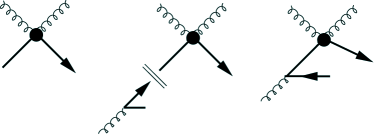
Figure 18: a) Generic leading-order diagram for flavor-excitation (LO-FE), $gQ\to gQ$. b) Subtraction diagram for flavor-excitation (SUB-FE), ${}^{1}f_{g\to Q}\otimes\sigma(gQ\to gQ)$. c) Next-to-leading-order diagram for flavor-creation (NLO-FC).

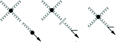
Figure 19: a) Generic leading-order diagram for flavor-fragmentation (LO-FF), $\sigma(gg\to gg)\otimes D_{g\to Q}$. b) Subtraction diagram for flavor-fragmentation (SUB-FF), $\sigma(gg\to gg)\otimes{}^{1}d_{g\to Q}$. c) Next-to-leading-order diagram for flavor-creation (NLO-FC).

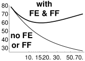
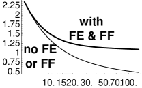
Figure 20: The differential cross section $d^{2}\sigma/dp_{T}^{2}/dy_{1}$ at $p_{T}=20,\,40\,GeV$ and $y_{1}=0$ in $(pb/GeV^{2})$ vs. $\mu$. The lower curves (thin line) are the heavy quark production cross sections ignoring flavor-excitation (FE) and flavor-fragmentation (FF). The upper curves (thick line) are the heavy quark production cross sections including FE and FF. Cf., Ref. [35].

Improved experimental measurements of heavy quark hadroproduction have increased the demand on the theoretical community for more precise predictions.[31] The first Next-to-Leading-Order (NLO) calculations of charm and bottom hadroproduction cross sections were performed some years ago.[32] As the accuracy of the data increased, the theoretical predictions displayed some shortcomings: 1) the theoretical cross-sections fell well short of the measured values, and 2) they displayed a strong dependence on the unphysical renormalization scale $\mu$. Both these difficulties indicated that these predictions were missing important physics.

One possible solution for these deficiencies was to consider contributions from large logarithms associated with the new quark mass scale, such as $\ln(s/m_{Q}^{2})$ and $\ln(p_{T}^{2}/m_{Q}^{2})$, Pushing the calculation to one more order, formidable as it is, would not improve the situation since these large logarithms persist to every order of perturbation theory. Therefore, a new approach was required to include these logs.

In 1994, Cacciari and Greco[34] observed that since the heavy quark mass played a limited dynamical role in the high $p_{t}$ region, one could instead use the massless NLO jet calculation convoluted with a fragmentation into a massive heavy quark pair to more accurately compute the production cross section in the region $p_{t}\gg m_{Q}$. In particular, they find that the dependence on the renormalization scale is significantly reduced, (cf., Fig. 17).

A recent study[35] investigated using initial-state heavy quark PDFs and final-state fragmentation functions to resum the large logarithms of the quark mass. The principle ingredient was to include the leading-order flavor-excitation (LO-FE) graph (Fig. 18) and the leading-order flavor-fragmentation (LO-FF) graph (Fig. 19) in the traditional NLO heavy quark calculation.[32] These contributions can not be added naively to the ${\cal O}(\alpha_{s}^{3})$ calculation as they would double-count contributions already included in the NLO terms; therefore, a subtraction term must be included to eliminate the region of phase space where these two contributions overlap. This subtraction term plays the dual role of eliminating the large unphysical collinear logs in the high energy region, and minimizing the renormalization scale dependence in the threshold region. The complete calculation including the contribution of the heavy quark PDFs and fragmentation functions 1) increases the theoretical prediction, thus moving it closer to the experimental data, and 2) reduces the $\mu$-dependence of the full calculation, thus improving the predictive power of the theory. (Cf., Fig 20.)

In summary, heavy quark hadroproduction is of interest experimentally because of the wealth of data allows precise tests of many different aspects of the theory, namely radiative corrections, resummation of logs, and multi-scale problems. Hence, this is a natural testing ground for QCD, and will allow us to extend the region of validity for the heavy quark calculation. This is an essential step necessary to bring theory in agreement with experiment.

6 SUMMARY

6.1 Kinematic Reach of Future Machines

Table 5: Future $ep$ collider machines chosen for study.

Index	Elepton	Eproton	$\sqrt{s}$	Machine(s)
	(Gev)	(Gev)	(Gev)
1	27	820	300	Hera
2	35	7,000	990	Lep $\times$ LHC
3	8	30,000	980	Low E lepton $\times$ 60 GeV pp
4	30	30,000	1900	Lep $\times$ 60 GeV pp
5	500	500	1000	NLC $\times$ conv. p
6	2,000	500	2000	$\mu$ collider $\times$ conv. p

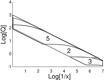
Figure 21: Kinematic reach of future facilities.

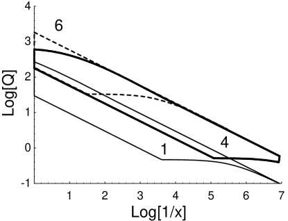
Figure 22: Kinematic reach of future facilities.

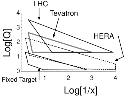
Figure 23: Kinematic reach of present and planned facilities. Note the full $\{x,Q^{2}\}$ region is clipped by the plot.

A central goal of this workshop was to study the physics potential of future facilities. Here, we focus on lepton-hadron colliders. We expand our study beyond the single $ep$ machine proposed in the workshop outline, and consider a mix of lepton and hadron beams from those proposed for the lepton-lepton and hadron-hadron options. The complete list is given in Table 5. To covert these parameters into the $\{x,Q^{2}\}$ range, we make use of:

$$y=1-\frac{E^{\prime}_{e}}{2E_{e}}(1-\cos\theta_{\ell})\quad,$$ (7)

$$Q^{2}=2E_{e}E^{\prime}_{e}(1+\cos\theta_{\ell})\quad,$$ (8)

and

$$x=Q^{2}/sy\quad.$$ (9)

For collider kinematics, we use

$$s\sim 4E_{e}E_{p}\quad.$$ (10)

Here, $E_{e}$ is the incoming lepton energy, $E^{\prime}_{e}$ is the outgoing lepton energy, $E_{p}$ is the incoming hadron energy, and $\theta_{\ell}$ is the lepton scattering angle.

To set practical limits on measurement of the final state, we impose:

• $y>0.01$  (resolution),

• $y<1$  (kinematic cut)

• $\theta_{\ell}>10^{\circ}$

• $\theta_{\ell}<179^{\circ}$

The constraint $\theta_{\ell}<179^{\circ}$ may be somewhat optimistic; if we relax this to $\theta_{\ell}\,\lower 2.15277pt\hbox{$\stackrel{{\scriptstyle<}}{{\sim}}$}\,176^{\circ}$, the result is to lose some of the low $Q$ region. The constraint $\theta_{\ell}>10^{\circ}$ has a relatively small effect; for the higher energy machines (e.g, 2 & 3), it clips the upper $Q$ region.

We display the kinematic reach for these proposed machines in Figs. 21 and 22. We include HERA for reference. In Fig. 21, we show the three machine options with a CMS of $\sqrt{s}\sim 1\,{\rm TeV}$. In Fig. 22, we show HERA and the remaining two machine options. In Fig. 23, we show the present and planned (LHC) facilities.

Although there is currently no plan to extract the primary beam to make a neutrino fixed target experiment at either the LHC or at a 2 TeV muon collider, there is a case to be made for doing precisely that. First of all, it would be very interesting to see if there were an anomalous rise in $xF_{3}$ similar to that seen in $F_{2}$ at HERA. Secondly, the low $x$ region of the Bjorken integral is anomalously large, and an outstanding question is, what is the very low $x$ behavior of the Gross-Llewellyn Smith integral ($xF_{3}$)? Either an experiment at the LHC or one at a 2 TeV muon collider could extend the range of the ”Fixed Target” region indicated in Figure 23 by an order of magnitude in the log ($1/x$) direction, assuming an order of magnitude higher neutrino energies than what CCFR/NuTeV has. The neutrino cross section would be an order of magnitude higher than the one applicable for CCFR/NuTeV, so good statistics are in principle attainable. Although these experiments would not have the kinematic reach to extremely low $x$ that $ep$ machines have, they can measure to high precision the non-singlet structure function, which at present has only been measured down to $x=.01$. In principle an ep machine running with both positive and negative leptons could do the same, but the luminosity requirements may be prohibitively high. We have still not learned all that we can learn from neutrino experiments, and even modest improvements in neutrino energies can uncover much new ground.

While we would of course like to probe the full $\{x,Q^{2}\}$ space, there are some particular reasons why the small $x$ region is of special interest. For example, the rapid rise of the $F_{2}$ structure function observed at HERA suggests that we may reach the parton density saturation region more quickly than anticipated. Additionally, the small $x$ region can serve as a useful testing ground for BFKL, diffractive phenomena, and similar processes. We can clearly see in Fig. 21 that with a fixed $\sqrt{s}$, we can best probe the small $x$ region with a high energy hadron beam colliding with a low energy lepton beam, and the loss in the high $Q$ region is minimal. From these (preliminary) studies, it would seem the optimal $ep$ facility would match the highest energy hadron beam available with a modest energy lepton beam.

References

- [1] H.L. Lai et al., Phys. Rev. D55, 1280-1296 (1997).
- [2] Space limitation prohibits a complete set of citations. See Ref. [1] for more detailed references.
- [3] NMC Collaboration: (M. Arneodo et al.) Phys. Lett. B364, 107 (1995); H1 Collaboration (S. Aid et al.): “1993 data”, Nucl. Phys. B439, 471 (1995); “1994 data”, Nucl. Phys. B470, 3-40 (1996); ZEUS Collaboration (M. Derrick et al.): “1993 data” Z. Phys. C65, 379 (1995) ; “1994 data”, DESY-96-076 (1996); E665 Collaboration (M.R. Adams et al.): FNAL-Pub-95/396-E, 1996.
- [4] CDF Collaboration Run-IA: (Abe et al.), Fermilab-PUB-96/020-E (1996) to appear in Phys. Rev. Lett., and Run-IB: B. Flaugher, Talk given at APS meeting, Indianapolis, May, 1996; D0 Collaboration: G. Blazey, Rencontre de Moriond, March, 1996; D. Elvira, Rome conference on DIS and Related Phenomena, April, 1996.
- [5] CTEQ Collaboration: J. Huston et.al., Phys. Rev. D 51, 6139 (1995).
- [6] S. Ellis, Z. Kunszt, and D. Soper, Phys. Rev. Lett. 64 2121 (1990); F. Aversa et al., Phys. Rev. Lett. 65, 401 (1990); W. Giele et al., Nucl. Phys. B403, 2121 (1993).
- [7] H.L. Lai, W.K. Tung, hep-ph/9605269; J. Huston, E. Kovacs, S. Kuhlmann, H.L. Lai, J.F. Owens, D. Soper, W.K. Tung, Phys. Rev. Lett. 77, 444 (1996).
- [8] E.W.N. Glover, et.al. Phys. Lett. B381, 353 (1996); A.D. Martin et.al. Phys. Lett. B387, 419 (1996).
- [9] H.L. Lai et al., Phys. Rev. D 51 4763 (1995).
- [10] F.J. Yndurain, e-Print Archive: hep-ph/9605265
- [11] J. Collins, W. Tung., Nucl.Phys. B278, 934 (1986).
- [12] CDF Collaboration: (Abe et al.), Fermilab-PUB-96/020-E (1996) to appear in Phys. Rev. Lett.
- [13] CDF Collaboration: B. Flaugher, Talk given at APS meeting, Indianapolis, May, 1996.
- [14] D0 Collaboration: J. Blazey, Talk given at Rencontre de Moriond, March, 1996; D. Elvira, Talk given at Rome conference on DIS and Related Phenomena, April, 1996.
- [15] A. Martin et al., Phys. Lett. B306, 145 (1993).
- [16] G. Altarelli and G. Parisi, Nucl. Phys. B126,298(1977).
- [17] D. A. Harris, W. G. Seligman et al., to appear in ICHEP-96 proceedings.
- [18] New Muon Collaboration (M. Arneodo et al.), Phys. Lett. B309,222(1993).
- [19] M. Virchaux and A. Milsztajn, PLB274,221(1992).
- [20] R. D. Ball and S. Forte Phys. Lett. B358,365(1995).
- [21] D.J. Gross and C.H. Llewellyn Smith, Nucl. Phys. B14 337 (1969)
- [22] J.D. Bjorken: Phys. Rev. 148,1467(1966), Phys. Rev. D1 1376 (1970).
- [23] J. Ellis, E. Gardi, M. Karliner, M. A. Samuel, Phys. Lett. B366,268 (1996).
- [24] CCFR Collaboration (D.A. Harris et al.), FERMILAB-CONF-95-144, Mar 1995. Appears in the 30th Rencontres de Moriond, 1995.
- [25] E142 Collaboration (P.L. Anthony et al.) SLAC-PUB-7103, Sep 1996, to be published in Phys. Rev. D.
- [26] Emlyn Hughes contribution to ICHEP-96 proceedings.
- [27] V.M. Braun and A. V. Kolesnichenko, Nucl. Phys. B283 723 (1987).
- [28] CDF Collaboration: Phys. Rev. Lett. 75, 11 (1995), Phys. Rev. D52, 4784 (1995).
- [29] Y.K. Kim, talk given at Snowmass
- [30] CDF Collaboration: Phys. Rev. Lett. 74, 850 (1995).
- [31] CDF Collaboration: V. Papadimitriou. FERMILAB-CONF-95-128-E. D0 Collaboration: L. Markosky. FERMILAB-CONF-95-137-E; Kamel A. Bazizi. FERMILAB-CONF-95-238-E.
- [32] P. Nason, ETH-PT/88-11. P. Nason, S. Dawson, R.K. Ellis, Nucl.Phys. B327, 49 (1989), Err.-ibid.B335, 260 (1990). ibid. B303, 607 (1988). M.L. Mangano, P. Nason, G. Ridolfi. ibid. B405, 507 (1993). W. Beenakker, H. Kuijf, W.L. van Neerven, J. Smith, PRD40, 54 (1989).
- [33] J. Collins, W. Tung., Nucl.Phys.B278, 934 (1986). F. Olness, W.-K. Tung, Nucl.Phys. B308, 813 (1988). M. Aivazis, F. Olness, W. Tung, Phys.Rev.Lett. 65, 2339 (1990). Phys.Rev. D50, 3085 (1994). M. Aivazis, J. Collins, F. Olness, W. Tung, Phys.Rev. D50, 3102 (1994).
- [34] M. Cacciari, M. Greco, Nucl.Phys.B421, 530 (1994). Z.Phys.C69, 459 (1996). B. Mele, P. Nason, Phys.Lett.B245, 635 (1990). Nucl.Phys.B361, 626 (1991).
- [35] F.I. Olness, R.J. Scalise, and W.-K. Tung, SMU-HEP-96/08; J.C. Collins, F.I. Olness, R.J. Scalise, and W.-K. Tung, CTEQ-616 (in preparation).