Hybrids and Quark Confinement

Abstract

It has become traditional to assume that the Dirac structure of the phenomenological quark confinement potential is scalar $\otimes$ scalar. We use the heavy quark expansion of the Coulomb gauge QCD Hamiltonian and the Flux Tube model to demonstrate that this is true but in the effective sense only. The demonstration contains some surprises: confinement is actually vector $\otimes$ vector and it is nonperturbative mixing between ordinary and hybrid $Q\bar{Q}$ states which generates the scalar-like spin dependent potential at order $1/m_{q}^{2}$. Thus the existence of hybrids is crucial to establishing well-known spin splitting phenomenology. Finally, the resolution also indicates that the gluonic degrees of freedom in a hybrid must be of a collective nature.

1 Introduction

Although it has been postulated for more than 30 years, the phenomenon of quark confinement remains an enigmatic feature of QCD. Quenched lattice gauge theory and heavy quark phenomenology indicate that the static ($m_{q}>>\Lambda_{QCD}$) long range potential should be linear with a slope of $b\approx 0.18\,{\rm GeV}^{2}$. The order $1/m_{q}^{2}$ quark-antiquark long range spin-dependent (SD) structure is also of interest and is the subject of this paper. In a model approach, ${Q\bar{Q}}$ interactions are typically derived from a nonrelativistic reduction of a relativistic current-current interaction

$$V_{conf}=\int j_{\Gamma}({\bf x})K({\bf x}-{\bf y})j_{\Gamma}({\bf y}).$$ (1)

In the heavy quark, nonrelativistic limit, this reduces to

$$V_{conf}\rightarrow\epsilon(r)+V_{SD}+\ldots$$ (2)

where the ellipsis denotes the spin independent interaction at ${\cal O}(1/m^{2})$ and terms of higher order in $1/m$. The spin dependent interaction may be parameterized as[1]

$$V_{SD}(r) = \left({{\sigma}_{q}\cdot{\bf L}_{q}\over 4m_{q}^{2}}-{{\sigma}_{\bar{q}}\cdot{\bf L}_{\bar{q}}\over 4m_{\bar{q}}^{2}}\right)\left({1\over r}{d\epsilon\over dr}+{2\over r}{dV_{1}\over dr}\right)+\left({{\sigma}_{\bar{q}}\cdot{\bf L}_{q}\over 2m_{q}m_{\bar{q}}}-{{\sigma}_{q}\cdot{\bf L}_{\bar{q}}\over 2m_{q}m_{\bar{q}}}\right)\left({1\over r}{dV_{2}\over dr}\right)$$ (3)

$$+{1\over 12m_{q}m_{\bar{q}}}\Big{(}3{\sigma}_{q}\cdot\hat{\bf r}\,{\sigma}_{\bar{q}}\cdot\hat{\bf r}-{\sigma}_{q}\cdot{\sigma}_{\bar{q}}\Big{)}V_{3}(r)+{1\over 12m_{q}m_{\bar{q}}}{\sigma}_{q}\cdot{\sigma}_{\bar{q}}V_{4}(r).$$

Here $\epsilon=\epsilon(r)$ is the static potential, $r=|{\bf r}_{q}-{\bf r}_{\bar{q}}|$ is the ${\bar{Q}Q}$ separation and the $V_{i}=V_{i}(r)$ are potentials which depend on the nonperturbative structure of QCD. Assuming that the $V_{i}$ simply follow from Eq. (1) yields the results shown in Table I [2]. Tensor and axial vector currents have spin-dependent static potentials and are therefore not useful for phenomenology in this context. Even the derivation of these simple results is beset with ambiguities and controversy. The reader is referred to the excellent review by Gromes in Ref. [2]. Finally we note that covariance under Lorentz transformations leads to a constraint between the SD potentials: $\epsilon(r)=V_{2}(r)-V_{1}(r)$, known as Gromes’ relation[3].

Table 1: Nonrelativisitic limits of Eq. (1).

$\Gamma$	$\epsilon_{\Gamma}$	$V_{1}$	$V_{2}$	$V_{3}$	$V_{4}$
scalar	$S$	$-S$	0	0	0
vector	$V$	0	$V$	$V^{\prime}/r-V^{\prime\prime}$	$2\nabla^{2}V$
pseudoscalar	0	0	0	$P^{\prime\prime}-P^{\prime}/r$	$\nabla^{2}P$

Twenty-two years ago Schnitzer[4] examined splittings in P-wave heavy quarkonia in an attempt to distinguish the possible spin dependence of the confinement potential. Specifically, he assumed a vector Coulomb short range potential and scalar or vector long range potentials. The ratio of P-wave splittings is then given by

$$\rho_{\buildrel V\over{S}}\equiv{M(^{3}P_{2})-M(^{3}P_{1})\over M(^{3}P_{1})-M(^{3}P_{0})}={\langle{16\alpha_{s}\over 5r^{3}}\pm A{b\over r}\rangle\over\langle{4\alpha_{s}\over r^{3}}\pm B{b\over 2r}\rangle},$$ (4)

where $A=14$ (1) and $B=4$ (1) for the vector (scalar) case. Experimentally, the splittings for the $J/\psi$ and $\Upsilon$ systems are 0.48 and 0.66 respectively. These are shown as horizontal lines in Fig. 1. The upper and lower curves are $\rho_{V}$ and $\rho_{S}$ respectively (these have not been convoluted with the wavefunctions). Since the $b\bar{b}$ wavefunction is smaller than the $c\bar{c}$, the curve must drop with increasing $r$ to fit the data. Clearly only scalar confinement meets this criterion. This conclusion has been supported by many other methods, including lattice gauge theory[5], Wilson loop calculations[6, 7], and flux tube models[8].

    

Figure 1: Scalar (s) and vector (v) spin splittings vs. the quark-antiquark radius.

A consistent picture of a QCD-generated effective scalar confinement interaction appears to be emerging. It is therefore disconcerting that attempts to build models which are “closer” to QCD (typically relativistic models) seem to require vector confinement. For example, scalar Salpeter equations do not have stable solutions[9] and it appears to be impossible to construct a BCS-like vacuum of QCD when scalar confinement is assumed[10, 11]. This is problematical if one wishes to dynamically generate constituent quark masses. Furthermore, attempts at modeling chiral pions will be hindered by the explicit lack of chiral symmetry in a scalar interaction. Finally, baryons anticonfine and colour singlet Tamm-Dancoff or RPA bound states are infrared divergent in a scalar potential[12].

This issue was resolved in Ref. [13] by first performing a Foldy-Wouthuysen reduction of the full Coulomb gauge Hamiltonian of QCD. This immediately establishes that the Dirac structure of confinement for heavy quarks is of a timelike-vector nature. Furthermore, the spin dependent structure of the long range force is determined by nonperturbative mixing of the $q\bar{q}$ states with hybrids. Finally, if one assumes a flux tube-like configuration of the gluonic component of the hybrids, a “scalar” spin-dependent potential emerges in a natural way.

2 Heavy Quark Expansion of $H_{QCD}$

Our starting point is the Coulomb gauge QCD Hamiltonian

$$H_{QCD}=\int d{\bf x}\psi^{\dagger}({\bf x})\left[-i{\alpha}\cdot\nabla+\beta m\right]\psi({\bf x})+H_{YM}+V_{C}-g\int d{\bf x}\psi^{\dagger}({\bf x}){\alpha}\cdot{\bf A}({\bf x})\psi({\bf x})$$ (5)

where

$$V_{C}={1\over 2}g^{2}\int d{\bf x}d{\bf y}\,{\cal J}^{-1}\rho^{a}({\bf x})V^{ab}({\bf x},{\bf y};A){\cal J}\rho^{b}({\bf y}),$$ (6)

$$V^{ab}({\bf x},{\bf y};A)=\langle{\bf x},a|(\nabla\cdot{\cal D})^{-1}(-\nabla^{2})(\nabla\cdot{\cal D})^{-1}|{\bf y},b\rangle,$$ (7)

and

$$H_{YM}={1\over 2}\int d{\bf x}\left[{\cal J}^{-1}{\Pi}({\bf x}){\cal J}{\Pi}({\bf x})+{\bf B}^{2}({\bf x})\right].$$ (8)

The degrees of freedom are the transverse gluon field ${\bf A}={\bf A}^{a}{\rm T}^{a}$, its conjugate momentum ${\Pi}={\Pi}^{a}{\rm T}^{a}$, and the quark field in the Coulomb gauge. The Faddeev-Popov determinant is written as ${\cal J}=\mbox{Det}[\nabla\cdot{\cal D}]$, with ${\cal D}^{ab}=\nabla\delta^{ab}-gf^{abc}{\bf A}^{c}$ being the covariant derivative in the adjoint representation, and the magnetic field is given by ${\bf B}^{a}=\nabla\times{\bf A}^{a}+gf^{abc}{\bf A}^{b}\times{\bf A}^{c}$. The static interaction $V_{C}$ is the nonabelian analog of the Coulomb potential. It involves the full QCD color charge density which has both quark and gluon components,

$$\rho^{a}({\bf x})=\psi^{\dagger}({\bf x}){\rm T}^{a}\psi({\bf x})+f^{abc}{\bf A}^{b}({\bf x})\cdot{\Pi}^{c}({\bf x}).$$ (9)

The most salient feature of the Coulomb gauge Hamiltonian is that all of the degrees of freedom are physical. This makes it especially useful for identifying the physical mechanisms which drive the spin splittings in heavy quarkonia.

2.1 The Foldy-Wouthuysen Transformation

We proceed by performing a Foldy-Wouthuysen transformation on the QCD Hamiltonian. This is done in complete analogy to the quantum mechanical case where an operator is constructed which removes the interactions between upper and lower components of the quark wave function order by order in the inverse quark mass, except that the unitary transformation is now constructed in Fock space. The resulting Hamiltonian is given by

$$H_{QCD}\to H_{FW} = \int d{\bf x}\left(m_{q}h^{\dagger}({\bf x})h({\bf x})-m_{\bar{q}}\chi^{\dagger}({\bf x})\chi({\bf x})\right)+H_{YM}+$$ (10)

$$V_{C}+H_{1}+H_{2}+\ldots,$$

$$H_{1} = {1\over 2m_{q}}\int d{\bf x}h^{\dagger}({\bf x})\left({\bf D}^{2}-g{\sigma}\cdot{\bf B}\right)h({\bf x})-(h\rightarrow\chi;m_{q}\rightarrow m_{\bar{q}}),$$ (11)

$$H_{2} = {1\over 8m_{q}^{2}}\int d{\bf x}h^{\dagger}({\bf x})g{\sigma}\cdot[{\bf E},\times{\bf D}]h({\bf x})+(h\rightarrow\chi;m_{q}\rightarrow m_{\bar{q}}).$$ (12)

In this expression $h=(1+\beta)\psi/2$ and $\chi=(1-\beta)\psi/2$ denote the upper and lower components of the quark wave function and correspond to the annihilation and creation operators of the heavy quark and antiquark respectively. The ellipsis denotes terms which are either of $O(1/m^{3})$ or are spin-independent at order $1/m^{2}$. Finally ${\bf D}=i\nabla+g{\bf A}$ is the covariant derivative in the fundamental representation.

2.2 The Static Potential

To leading order in the quark mass the Hamiltonian describes two static, noninteracting quarks. At ${\cal O}(m^{0})$ the Hamiltonian reduces to $H_{0}=H_{YM}+V_{C}$. The eigenstates of $H_{0}$ may be labeled by the quark and antiquark coordinates and by an index which classifies the adiabatic state of the gluonic degrees of freedom, $n_{r}$,

$$H_{0}|n_{r};{\bf r}_{q}{\bf r}_{\bar{q}}\rangle=\epsilon_{n}(r)|n_{r};{\bf r}_{q}{\bf r}_{\bar{q}}\rangle.$$ (13)

Note that we have made explicit the dependence of the gluonic degrees of freedom on the position of the quarks, $r$.

The corresponding eigenenergies, $\epsilon_{n}(r)$ may be identified with the Wilson loop potentials calculated on the lattice. Thus for example, $\epsilon_{0}(r)$ is the Coulomb plus linear potential seen long ago. Static hybrid states are collectively denoted $|n_{r};{\bf r}_{q}{\bf r}_{\bar{q}}\rangle$ with $n_{r}\neq 0$. In recent studies [14] (see Fig. 2) the lowest lying adiabatic hybrid potential, $\epsilon_{1}(r)$ has been evaluated.

    

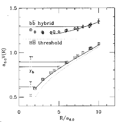
Figure 2: $\epsilon_{0}(R)$ (squares) and $\epsilon_{1}(R)$ (circles and diamonds). From Ref. 14.

While both $H_{YM}$ and $V_{C}$ may contribute to the linearly rising potential energy seen on the lattice, it is clear that the quarks may only interact with the flux tube via the nonabelian Coulomb interaction. Therefore the Dirac structure of confinement corresponds to $\gamma_{0}\otimes\gamma_{0}$ from the product of color charge densities (see Eqs. (6) and  (9)). As stressed in the Introduction, this appears to be at odds with 20 years of quark model phenomenology. Since the phenomenology is based on spin splittings, it will be instructive to examine the $1/m^{2}$ perturbative corrections to the static potential.

2.3 Spin-dependent Potentials

The spin-dependent first order correction to the static potential is given by $\delta\epsilon_{n}^{(1)}(r)=\langle n_{r};{\bf r}_{q}{\bf r}_{\bar{q}}|H_{2}|n_{r};{\bf r}_{q}{\bf r}_{\bar{q}}\rangle$. The order $1/m$ term is not considered because ${\bf D}^{2}$ is not spin-dependent and the matrix element of ${\sigma}\cdot{\bf B}$ vanishes. Evaluating this yields the standard classical plus Thomas precession spin orbit interaction

$$\delta\epsilon_{n}^{(1)}=\left({{\sigma}_{q}\cdot{\bf L}_{q}\over 4m_{q}^{2}}-{{\sigma}_{\bar{q}}\cdot{\bf L}_{\bar{q}}\over 4m_{\bar{q}}^{2}}\right){1\over r}{d\epsilon_{n}\over dr}.$$ (14)

Thus the first term in Eq. (3), generalized to any adiabatic potential and therefore true for both ordinary and hybrid $\bar{Q}Q$ states, is reproduced. Further SD corrections occur at second order in perturbation theory in $H_{1}$. This is shown diagramatically in Fig. 3. As indicated in the figure, $H_{1}$ contains two operators, $D^{2}$ and $\sigma\cdot{\bf B}$ which may act on quark or antiquark lines. The shaded blobs represent mixing via intermediate states which must be heavy quark hybrids. In Fig. 3a $\sigma\cdot{\bf B}$ acts on a single quark line and therefore does not yield a spin-dependent contribution to $V_{SD}$. Fig. 3b, alternatively, yields $V_{3}$ and $V_{4}$; while Figs. 3c and 3d give $V_{1}$ and $V_{2}$ respectively.

Thus, the application of the Foldy-Wouthuysen transformation to the Coulomb gauge QCD Hamiltonian shows that the spin-dependent effective potential may be simply interpreted as nonperturbative mixing with hybrid states. This makes it clear that it is possible for nonperturbative dynamical physics to generate an effective spin-dependent interaction which mimics a scalar interaction. Actually demonstrating this requires that the matrix elements be evaluated.

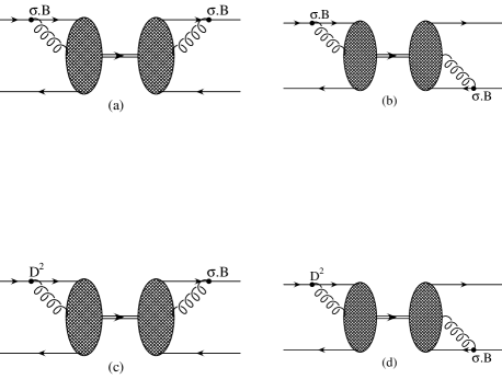
Figure 3: Contributions to the second order energy shift.

3 Model Evaluation of the Spin-dependent Potentials

Before proceeding to a model evaluation of the matrix elements we note that it is possible to make some general statements on their expected properties. The results of lattice gauge theory make it clear that a flux tube-like configuration of glue exists between static quarks. If one thinks of this as a localized object with an infinite number of degrees of freedom, then it is apparent that $V_{2}$ must evaluate to zero. This is because the electric field operator creates a local excitation in the flux tube at position ${\bf r}_{q}$ (see Fig. 3d). This must then be de-excited at ${\bf r}_{\bar{q}}$ by the magnetic field operator. However, the two operators become decorrelated because infinitely many degrees of freedom intervene. Similarly, the long range portions of $V_{3}$ and $V_{4}$ both vanish. Thus, by Gromes’ relation, the only nonzero long range interaction must be given by $V_{1}=-\epsilon$. This is precisely the situation required for “scalar” confinement. It is therefore entirely plausible that an effective scalar confinement is generated by nonperturbative mixing with hybrids. Furthermore, the structure of the spin-dependent terms depends crucially on the nature of the ground state gluonic degrees of freedom and clearly favors a collective rather than a single particle picture of them.

These simple expectations are borne out in an explicit model calculation[13] where the Flux Tube Model of Isgur and Paton [15] was used to evaluate the relevant matrix elements. The interested reader is referred to Ref. [13] for details. Evaluating the spin dependent potentials in the Flux Tube Model requires explicit expressions for the electric and magnetic fields in a flux tube. It was therefore necessary to extend the Flux Tube Model somewhat. Here I take the opportunity to correct some typos in Ref. [13].

The commutation relation between the electric and magnetic fields is

$$[E^{a}_{i}({\bf x}),B^{b}_{j}({\bf y})]=i\epsilon^{ijk}\nabla^{k}_{y}\delta({\bf y}-{\bf x})\delta^{ab}+{\cal O}(g),$$ (15)

which implies that the electric and magnetic field operators may be defined in terms of the transverse string coordinate $\chi$ as

$$E^{a}_{\lambda}(n)\sim{\kappa\over a^{3}}(\chi^{a}_{\lambda}(n+1)-\chi^{a}_{\lambda}(n))$$ (16)

and

$$B^{a}_{\lambda}(n)={-i\over\kappa a}{\partial\over\partial\chi^{a}_{\bar{\lambda}}(n)}.$$ (17)

Here $\kappa=a\sqrt{b_{0}}$ and the $\epsilon^{ijk}$ of the commutator in Eq. (15) is taken into account by the index $\bar{\lambda}$, $\chi_{\bar{x}}(n)=\chi_{y}(n)$ and $\chi_{\bar{y}}(n)=-\chi_{x}(n)$.

This corrects several sign errors in Ref. [13]. Note also that Eq. 38 of that paper should be in terms of $\bar{\lambda}$ not $\lambda$. None of the results are changed.

Finally, evaluating the matrix elements from the perturbative expansion yields

$$V_{1}(r)=-{g^{2}\over 2a^{2}}C_{F}r$$ (18)

and

$$V_{2}(r)=\lim_{N\rightarrow\infty}{g^{2}\over 2a^{2}}C_{F}{r\over N}.$$ (19)

In the strong coupling limit one has $b=g^{2}/(2a^{2})C_{F}$ so that the anticipated expression for $V_{1}$ emerges in a natural way. Furthermore, $V_{2}$ approaches zero like $1/N$; this is also true for $V_{3}$ and $V_{4}$. The latter point is illustrated in Fig. 4 where the correlation of electric and magnetic fields versus separation along the flux tube is shown. As expected the fields become completely decorrelated as the number of intervening degrees of freedom becomes large. Notice that this implies that a constituent gluon model of hybrids would not have been able to produce an effective scalar interaction.

Figure 4: Field Correlation Functions (for N=100).

4 Conclusions

Spin splittings and lattice calculations indicate that confinement is scalar in nature. This conflicts with many relativistic models of QCD which require vector confinement. For example, a chirally symmetric interaction is needed if pseudo-Goldstone pions and spontaneous chiral symmetry breaking are to be generated dynamically. Furthermore it appears to be impossible to build a stable vacuum with a scalar kernel. We have examined this issue with the heavy quark limit of the Coulomb gauge QCD Hamiltonian. This approach is physically intuitive and is simpler to interpret and implement than methods based on the Wilson loop. We found that the static confinement potential must indeed be a Dirac timelike vector. Effective scalar interactions are generated at order $1/m^{2}$ by nonperturbative mixing with hybrid states.

We have argued that the long range spin-spin ($V_{3}$ and $V_{4}$) and the vector-like spin-orbit potentials ($V_{2}$) should all be zero since they involve field correlation functions evaluated between quark and antiquark. This statement follows by assuming that the gluonic degrees of freedom collapse into a flux tube-like configuration, as shown by lattice gauge theory. Alternatively, the scalar-like spin-orbit potential ($V_{1}$) is proportional to the matrix element of the electric and magnetic fields evaluated at the same point and hence is expected to be nonzero. Explicit calculations of the relevant matrix elements were carried out in the Flux Tube Model. The model was extended to include color degrees of freedom and to map the chromoelectric and chromomagnetic fields to flux tube phonon operators. The results obtained were in agreement with our general arguments and with Gromes’ relation.

A consistent picture of the Dirac structure of confinement has emerged. The static central potential is timelike vector while the spin-dependent structure mimics the nonrelativistic reduction of an effective scalar interaction. This implies that it is incorrect to employ a scalar confinement kernel when doing calculations with light quarks. Note however that it would be acceptable to use scalar confinement when working explicitly in the chiral symmetry broken phase, i.e., with constituent quarks in the nonrelativistic limit. The work presented here also implies that a constituent gluon picture of hybrids will yield incorrect results for certain observables. For example, $V_{1}$ and $V_{2}$ would be of comparable magnitude in a constituent gluon model. In general, these types of models must fail when nonlocal properties of the gluonic configuration are considered. Alternatively, it is possible that they perform quite well when evaluating global properties of gluonics such as the hybrid spectrum.

References

References

- [1] E. Eichten and F. Feinberg, Phys. Rev. D23, 2724 (1981).
- [2] W. Lucha, F. F. Schöberl, and D. Gromes, Phys. Rep. 200, 127 (1991).
- [3] D. Gromes, Z. Phys. C11, 147 (1981); erratum C14, 94 (1982).
- [4] H.J. Schnitzer, Phys. Rev. Lett. 35, 1540 (1975).
- [5] C. Michael, Phys. Rev. Lett. 56, 1219 (1986).
- [6] E. Montaldi, A. Burchielli, and G.M. Prosperi, Nucl. Phys. B296, 625 (1988); M. Baker, J.S. Ball, N. Brambilla, G.M. Prosperi, and F. Zachariasen, Phys. Rev. D54, 2829 (1996); Yu.A. Simonov, Nucl. Phys. B324, 67 (1989).
- [7] N. Brambilla, P. Consoli, and G. M. Prosperi, Phys. Rev. D50, 5878 (1994).
- [8] W. Buchmüller, Phys. Lett. 112B, 479 (1982). For extensions of this idea see M.G. Olsson, S. Veseli, and K. Williams, Phys. Rev. D53, 4006 (1996) and references therein.
- [9] J. Parramore and J. Piekarewicz, Nucl. Phys. A585, 705 (1995). See also J. Resag and C.R. Münz, Nucl. Phys. A590, 735 (1995).
- [10] A. Szczepaniak, E.S. Swanson, C.-R. Ji, and S.R. Cotanch, Phys. Rev. Lett. 76, 2011 (1996).
- [11] A.P. Szczepaniak and E.S. Swanson, Phys. Rev. D55, 1578 (1997).
- [12] A.P. Szczepaniak and E.S. Swanson, unpublished.
- [13] A.P. Szczepaniak and E.S. Swanson, Phys. Rev. D55, 3987 (1997).
- [14] S. Perantonis and C. Michael, Nucl. Phys. B347, 854 (1990).
- [15] N. Isgur and J. Paton, Phys. Rev. D31, 2910 (1985).