MPI/PhT/97–032
hep-ph/9706462
May 1997

Complete QCD Corrections of Order ${\cal O}(\alpha_{s}^{3})$ to the Hadronic Higgs Decay

Abstract

We consider the decay of an intermediate mass Higgs boson into hadrons up to order ${\cal O}(\alpha_{s}^{3})$. The results from the diagrams containing only light degrees of freedom were recently computed in a previous work by K.G. Ch. (Phys. Lett. B 390 (1997) 309). In this letter the remaining contributions involving the top quark are evaluated analytically using an effective field theory approach. Coupled with the previous result the present calculation determines the complete next-next-to-leading order correction to the hadronic decay rate of an intermediate mass Higgs boson.

The Higgs boson is the only still missing particle in the standard model of particle physics. Up to now only mass limits exist from the failure of experiments at the CERN Large Electron-Positron Collider (LEP1) to observe the process $e^{+}e^{-}\to ZH$. Currently the mass range $M_{H}\leq 65.6$ GeV is ruled out at the 95% confidence level [1].

From the theoretical side a lot of effort has been invested to get more insight into the properties of the Higgs boson (for a review see [2]). Of particular interest is thereby the intermediate mass range where $m_{b}\ll M_{H}\;\hbox to0.0pt{\lower 3.5pt\hbox{$\mathchar 0\relax\sim$}\hss}\raise 1.0pt\hbox{$<$}\;2M_{W}$. Then the dominant decay mode is the one into bottom quarks. Concerning QCD corrections the full mass dependence at ${\cal O}(\alpha_{s})$ was evaluated in [3]. However, especially for the fermionic decay of an intermediate mass Higgs boson it turns out that an expansion in the quark masses provides reasonable approximations. At ${\cal O}(\alpha_{s}^{2})$ besides the massless limit (i.e. keeping only the overall factor $m_{b}^{2}$) [4] also subleading mass corrections in the $m_{b}^{2}/M_{H}^{2}$ expansion are known [5, 6].

Recently the contribution to the scalar polarization function of the Higgs boson containing only light quarks was considered at four loops [7]. Its imaginary part was evaluated analytically in the massless limit leading to corrections of ${\cal O}(\alpha_{s}^{3})$ to the Higgs decay rate. The corresponding corrections prove to be numerically more important than the power suppressed contribution of ${\cal O}(\alpha^{2}_{s}m_{b}^{2}/M_{H}^{2})$.

In Ref. [6] additional quasi-massless (and numerically important) contributions of order $\alpha_{s}^{2}$ have been identified and elaborated. They come from so-called singlet diagrams with a non-decoupling top quark loop inside. The results of Ref. [6] have been confirmed and extended by the computation of power-suppressed terms of order $\alpha_{s}^{2}(M_{H}^{2}/M_{t}^{2})^{n}\,(n=1,2,\ldots)$ [9]. For completeness we should mention that the exact result for the imaginary part of the double-bubble diagram with massless external quark and internal top quark can be found in [10]. Radiative corrections enhanced by a factor $M_{t}^{2}$, usually expressed through $X_{t}=G_{F}M_{t}^{2}/8\pi^{2}\sqrt{2}$, are also available up to the three-loop order [11, 12] and will be compared at the end with the new terms of ${\cal O}(\alpha_{s}^{3})$.

In this letter we calculate the top-induced corrections at ${\cal O}(\alpha_{s}^{3})$ and hence complete the analysis of the hadronic Higgs decay at NNNLO, as far as one neglects power suppressed corrections. Although the phenomenological interesting decay is the one into bottom quarks the following discussion will be kept more general and a generic light quark $q$ will be considered. However, for the numerical discussion we will come back to the case of bottom quarks.

We start with the bare Yukawa Lagrangian,

$${\cal L}_{Y}=-\frac{H^{0}}{v^{0}}\left(\sum_{q}m_{q}^{0}\bar{q}^{0}q^{0}+m_{t}^{0}\bar{t}^{0}t^{0}\right){},$$ (1)

where $v$ is the Higgs vacuum-expectation value and the superscript 0 labels bare quantities. Assuming that the Higgs boson mass, $M_{H}$ is less than the top quark mass $m_{t}$, ${\cal L}_{Y}$ can be replaced by an effective Lagrangian produced by integrating out the top quark field. According to Refs. [13, 12, 14] the resulting Lagrangian reads

$${\cal L}_{Y}^{\rm eff} = -\frac{H^{0}}{v^{0}}\left[C_{1}\left[O_{1}^{\prime}\right]+\sum_{q}C_{2q}\left[O_{2q}^{\prime}\right]\right],$$ (2)

where $[O_{1}^{\prime}]$ and $[O_{2q}^{\prime}]$ are the renormalized counterparts of the bare operators

$$O_{1}^{\prime}\,\,=\,\,\left(G_{a\mu\nu}^{0\prime}\right)^{2}, O_{2q}^{\prime}\,\,=\,\,m_{q}^{0\prime}\bar{q}^{0\prime}q^{0\prime},$$

with $G_{a\mu\nu}^{0\prime}$ being the (bare) field strength tensor of the gluon. The primes mark the quantities defined in the effective $n_{f}=5$ QCD including only light (in comparison to the top quark) $u,d,s,c$ and $b$ quarks. All the dependence on the top quark gets localized in the coefficient functions $C_{1}$ and $C_{2q}$. If the latter are known the computation of the total decay rate $\Gamma_{H}=\Gamma(H\to\mbox{hadrons})$ is reduced to the evaluation of the functions $\Delta_{jk}(M_{H}^{2})$ ($jk=11,12,22$) related via the optical theorem to the absorptive parts of the scalar correlators

$$\Pi_{jk}(q^{2})=i\int dxe^{iqx}\langle 0|\;T[\;O^{\prime}_{j}(x)O^{\prime}_{k}(0)\,]\;|0\rangle\bigg{|}_{q^{2}=M_{H}^{2}}{}.$$ (3)

It should be stressed that by the very meaning of the effective Lagrangian (2) the correlators of Eq. (3) may be computed within the effective massless QCD, which leads to a drastic simplification of the calculation. In addition, the coefficient functions $C_{1}$ and $C_{2q}$ essentially depend on only one kinematical variable, the top quark mass, which also simplifies their calculation a lot.

Typical diagrams contributing to $\Delta_{22}^{q}$, $\Delta_{11}$ and $\Delta_{12}^{q}$ are shown in Figs. 1-3. Note that every massless diagram contributing to $\Delta_{22}^{q}$ to order $\alpha_{s}^{3}$ does only have cuts containing at least one quark-antiquark pair. This allows one to unambiguously associate $\Delta^{q}_{22}$ to $\Gamma(H\to q\bar{q})$ — the partial decay rate of the Higgs boson to hadrons containing at least one $q\bar{q}$ pair. The diagrams contributing to $\Delta_{11}$ (see Fig. 2) describe the production of gluons. The leading order diagram has clearly only contributions to the $gg$ final state. Starting from NLO, however, there are contributions from diagrams leading both to $gg$, $ggg$ and $gq\bar{q}$ final states. The interpretation of the $\Delta_{12}^{q}$ (see Fig. 3) is even more complicated. Here different final states begin to appear already in the leading non-vanishing order [6]. In this paper we will adopt a pragmatical point of view and evaluate the total hadronic decay rate without any attempt to differentiate between final states [15].

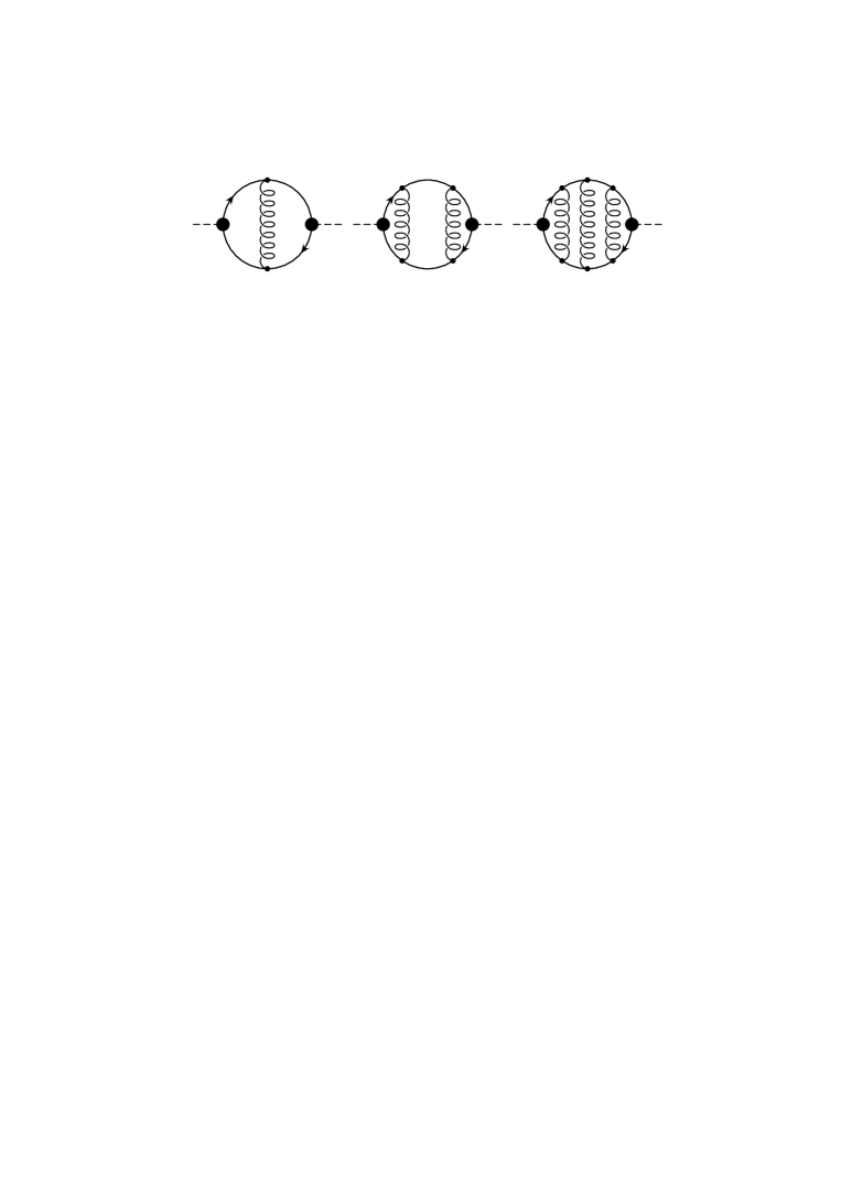
Figure 1: Typical Feynman diagrams contributing to $\Delta_{22}^{q}$. The solid circles represent the operator $\left[O_{2q}^{\prime}\right]$.

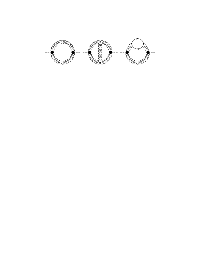
Figure 2: Typical Feynman diagrams contributing to $\Delta_{11}^{q}$. The solid circles represent the operator $\left[O_{1}^{\prime}\right]$.

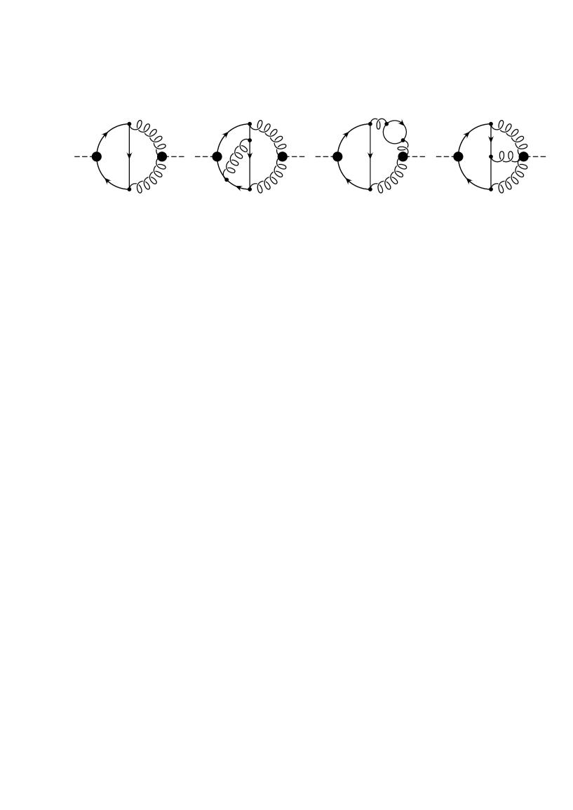
Figure 3: . Two- and some of the three-loop diagrams contributing to $\Delta_{12}^{q}$. The solid circles represent the operators $\left[O_{1}^{\prime}\right]$ and $\left[O_{2q}^{\prime}\right]$, respectively.

The functions $\Delta_{11}$, $C_{1}$ and $\Delta_{22}^{q}$ have been computed analytically in [13, 16, 14] and [7]. Thus, to complete the evaluation of $\Gamma_{H}$ in the ${\cal O}(\alpha_{s}^{3})$ approximation one needs to compute $C_{2q}$ as well as $\Delta_{12}^{q}$. This calculation and its results are described below.

For convenience we should recall the relevant formulae which connect the bare and renormalized quantities appearing in Eq. (2). For the operators we have

$$\left[O_{1}^{\prime}\right] = \left[1+2\left(\frac{\alpha_{s}\partial}{\partial\alpha_{s}}\ln Z_{g}\right)\right]O_{1}^{\prime}-4\left(\frac{\alpha_{s}\partial}{\partial\alpha_{s}}\ln Z_{m}\right)\sum_{q}O_{2q}^{\prime},$$

$$\left[O_{2q}^{\prime}\right] = O_{2q}^{\prime},$$ (4)

and for the coefficient function the relations look like:

$$C_{1} = \frac{1}{1+2(\alpha_{s}\partial/\partial\alpha_{s})\ln Z_{g}}C_{1}^{0},$$

$$C_{2q} = \frac{4(\alpha_{s}\partial/\partial\alpha_{s})\ln Z_{m}}{1+2(\alpha_{s}\partial/\partial\alpha_{s})\ln Z_{g}}C_{1}^{0}+C_{2q}^{0},$$ (5)

where the renormalization constant $Z_{g}$ and $Z_{m}$ are defined in the effective theory. In the order we are interested in these constants are needed up the one- and two-loop level, respectively, because $C_{1}^{0}$ is already proportional to $\alpha_{s}$.

For our purpose we need $C_{1}$ up to order $\alpha_{s}^{2}$ which may be found in [13, 16, 14]. $C_{2q}$ is also known up to ${\cal O}(\alpha_{s}^{2})$ [12] but for the present analysis needed up to ${\cal O}(\alpha_{s}^{3})$. To this aim we want to use the low energy theorem (LET) which allows to attach the Higgs boson via differentiation w.r.t. the masses involved in the process. The formula given in [12] for the computation of $C_{2q}^{0}$ simplifies in our case to

$$C_{2q}^{0} = 1-\frac{m_{t}^{0}\partial}{\partial m_{t}^{0}}\left(\Sigma_{S}^{0t}(0)+\Sigma_{V}^{0t}(0)\right).$$ (6)

It is understood that after the derivative w.r.t. the bare top mass is done the renormalization of the parameters $m_{t}$ and $\alpha_{s}$ is performed. The superscript $t$ indicates that only the diagrams where at least one top quark is present have to be taken into account. The first non-vanishing contribution arises at two-loop level involving one diagram. At three loops altogether 25 diagrams contribute. Some typical examples are depicted in Fig. 4.

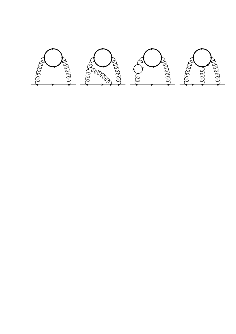
Figure 4: Two- and some of the three-loop diagrams contributing to $\Sigma_{S}^{0t}$ and $\Sigma_{V}^{0t}$. The thick (thin) lines represents the top quark (light quarks).

Note that only the pole parts have to be computed because the integrals are logarithmically divergent and consequently proportional to $(\mu^{2}/m_{t}^{2})^{\varepsilon}$. The differentiation w.r.t. the top mass then leads to an additional factor $\varepsilon$. The diagrams are generated with the program QGRAF [17] and fed into the package MATAD written in FORM [18] for the purpose to solve three-loop tadpole integrals. The calculation was performed with arbitrary QCD gauge parameter $\xi$. $\Sigma_{S}^{0t}$ and $\Sigma_{V}^{0t}$ separately still depend on $\xi$, however, the final result for $C_{2q}$ is independent of the gauge parameter which serves as a welcome check. Expressing the result in terms of the $\overline{\mbox{MS}}$ top mass, $m_{t}$, we get

$$C_{2q} = 1+\left(\frac{\alpha_{s}^{(6)}(\mu)}{\pi}\right)^{2}\left[\frac{5}{18}-\frac{1}{3}\ln\frac{\mu^{2}}{m_{t}^{2}}\right]+\left(\frac{\alpha_{s}^{(6)}(\mu)}{\pi}\right)^{3}\left[\frac{311}{1296}+\frac{5}{3}\zeta(3)\right.$$ (7)

$$\left.\quad\mbox{}-\frac{175}{108}\ln\frac{\mu^{2}}{m_{t}^{2}}-\frac{29}{36}\ln^{2}\frac{\mu^{2}}{m_{t}^{2}}+n_{l}\left(\frac{53}{216}+\frac{1}{18}\ln^{2}\frac{\mu^{2}}{m_{t}^{2}}\right)\right],$$

with $\zeta(3)\approx 1.20206$. $n_{l}$ is the number of light quarks. Using the relation between the $\overline{\mbox{MS}}$ and the on-shell mass, $M_{t}$, at one-loop level, $m_{t}/M_{t}=1-(4/3+\ln\mu^{2}/M_{t}^{2})\alpha_{s}/\pi$, one gets:

$$C_{2q}^{OS} = 1+\left(\frac{\alpha_{s}^{(6)}(\mu)}{\pi}\right)^{2}\left[\frac{5}{18}-\frac{1}{3}\ln\frac{\mu^{2}}{M_{t}^{2}}\right]+\left(\frac{\alpha_{s}^{(6)}(\mu)}{\pi}\right)^{3}\left[-\frac{841}{1296}+\frac{5}{3}\zeta(3)\right.$$ (8)

$$\left.\quad\mbox{}-\frac{247}{108}\ln\frac{\mu^{2}}{M_{t}^{2}}-\frac{29}{36}\ln^{2}\frac{\mu^{2}}{M_{t}^{2}}+n_{l}\left(\frac{53}{216}+\frac{1}{18}\ln^{2}\frac{\mu^{2}}{M_{t}^{2}}\right)\right],$$

For completeness we also list the result for $C_{1}$ [13, 16, 14]:

$$C_{1} = -\frac{1}{12}\,\frac{\alpha_{s}^{(6)}(\mu)}{\pi}\left[1+\frac{\alpha_{s}^{(6)}(\mu)}{\pi}\left(\frac{11}{4}-\frac{1}{6}\ln\frac{\mu^{2}}{m_{t}^{2}}\right)\right].$$ (9)

On the basis of the effective Lagrangian of Eq. (2) it is possible to write down the decay rate of the Higgs boson into hadrons in the following form:

$$\Gamma\left(H\to\mbox{hadrons}\right) = \left(1+\delta_{u}\right)^{2}\bigg{\{}\sum_{q}A_{q\bar{q}}\left[\left(1+\Delta^{q}_{22}\right)\left(C_{2q}\right)^{2}+\Delta^{q}_{12}\,C_{1}C_{2q}+\Delta^{\rm hdo}\right]$$ (10)

$$\mbox{}\qquad\qquad+A_{gg}\,\Delta_{11}\,\left(C_{1}\right)^{2}\bigg{\}},$$

with $A_{q\bar{q}}=3G_{F}M_{H}m_{q}^{2}/4\pi\sqrt{2}$ and $A_{gg}=4G_{F}M_{H}^{3}/\pi\sqrt{2}$. The universal corrections $\delta_{u}$ arise from the renormalization of the factor $H^{0}/v^{0}$. The terms up to ${\cal O}(\alpha_{s}^{2}X_{t})$ can be found in [11]. $\Delta^{\rm hdo}$ summarizes the corrections coming from higher dimensional operators. They are at least suppressed by a factor $\alpha_{s}^{2}M_{H}^{2}/M_{t}^{2}$. The factors $\Delta_{ij}$ contain the electroweak and QCD corrections from the light degrees of freedom only. As we are interested up to an accuracy of ${\cal O}(\alpha_{s}^{3})$ $\Delta_{11}$ and $\Delta^{q}_{22}$ are known. However, $\Delta_{12}^{q}$ is only available at the two-loop level where one diagram has to be evaluated (see Fig. 3). We have to extend the analysis to three loops where altogether 28 massless three-loop diagrams have to be computed. This was done with the help of the program package MINCER [19]. In Fig. 3 some graphs are pictured. The single diagrams again depend on $\xi$ which cancels in the proper sum. The result reads:

$$\Delta^{q}_{12} = \frac{\alpha_{s}^{(5)}(\mu)}{\pi}\left[-\frac{92}{3}-8\ln\frac{\mu^{2}}{M_{H}^{2}}\right]$$ (11)

$$+\left(\frac{\alpha_{s}^{(5)}(\mu)}{\pi}\right)^{2}\left[-\frac{15073}{18}+76\zeta(2)+156\zeta(3)-\frac{1028}{3}\ln\frac{\mu^{2}}{M_{H}^{2}}-38\ln^{2}\frac{\mu^{2}}{M_{H}^{2}}\right.$$

$$\left.\mbox{}+n_{l}\left(\frac{283}{9}-\frac{8}{3}\zeta(2)-\frac{16}{3}\zeta(3)+\frac{112}{9}\ln\frac{\mu^{2}}{M_{H}^{2}}+\frac{4}{3}\ln^{2}\frac{\mu^{2}}{M_{H}^{2}}\right)\right],$$

with $\zeta(2)=\pi^{2}/6$. The ${\cal O}(\alpha_{s})$ terms can also be found in [6, 9, 12], the ${\cal O}(\alpha_{s}^{2})$ terms are new.

Let us now compare the new results of ${\cal O}(\alpha_{s}^{3})$ with the previous ones and also with other known correction terms which might be of the same order of magnitude. Here, we have in mind terms of order $\alpha_{s}^{2}m_{b}^{2}/M_{H}^{2}$, $\alpha\alpha_{s}$, $\alpha_{s}^{2}X_{t}$ and $\alpha_{s}^{2}M_{H}^{2}/M_{t}^{2}$. Thereby it is convenient to write Eq. (10) in the form:

$$\Gamma(H\to\mbox{hadrons}) = A_{b\bar{b}}\left(1+\Delta^{b}_{l}+\Delta_{t}\right)+\left(1+\delta_{u}\right)^{2}A_{gg}\,\Delta_{11}\,\left(C_{1}\right)^{2},$$ (12)

where $\Delta_{l}^{b}$ contains only corrections form light degrees of freedom and all top-induced terms from the first line of Eq. (10) are contained in $\Delta_{t}$. Furthermore we express $\Delta_{t}$ also in terms of $\alpha_{s}^{(5)}(\mu)$. Choosing $\mu^{2}=M_{H}^{2}$ and $n_{l}=5$ we find

$$\Delta_{l}^{b} = -6\frac{(m_{b}^{(5)})^{2}}{M_{H}^{2}}+0.472\,\frac{\bar{\alpha}(M_{H})}{\pi}+0.651\,\frac{\bar{\alpha}(M_{H})}{\pi}a_{H}^{(5)}+a_{H}^{(5)}\left(5.667-40.000\frac{(m_{b}^{(5)})^{2}}{M_{H}^{2}}\right)$$ (13)

$$\mbox{}+\left(a_{H}^{(5)}\right)^{2}\left(29.147-87.725\frac{(m_{b}^{(5)})^{2}}{M_{H}^{2}}\right)+41.758\left(a_{H}^{(5)}\right)^{3},$$

$$\Delta_{t} = \left(a_{H}^{(5)}\right)^{2}\left(3.111-0.667\,L_{t}+\frac{(m_{b}^{(5)})^{2}}{M_{H}^{2}}\left(-10+4\,L_{t}+\frac{4}{3}\ln\frac{(m_{b}^{(5)})^{2}}{M_{H}^{2}}\right)\right)$$ (14)

$$\mbox{}+\left(a_{H}^{(5)}\right)^{3}\left(50.474-8.167\,L_{t}-1.278\,L_{t}^{2}\right)+\left(a_{H}^{(5)}\right)^{2}\frac{M_{H}^{2}}{M_{t}^{2}}\left(0.241-0.070\,L_{t}\right)$$

$$\mbox{}+X_{t}\left(1-4.913a_{H}^{(5)}+\left(a_{H}^{(5)}\right)^{2}\left(-72.117-20.945\,L_{t}\right)\right),$$

with $a_{H}^{(5)}=\alpha_{s}^{(5)}(M_{H})/\pi$ and $L_{t}=\ln M_{H}^{2}/M_{t}^{2}$. The term in Eq. (14) proportional to $M_{H}^{2}/M_{t}^{2}$ is the leading contribution from $\Delta^{\rm hdo}$. The $(m_{b}^{(5)})^{2}/M_{H}^{2}$ corrections in $\Delta_{t}$ arise from the singlet diagram with one top and one bottom quark triangle and can be found in [6]. At this point we should mention that still contributions with pure gluonic final states are contained in Eq. (10). At ${\cal O}(\alpha_{s}^{3})$, however, these corrections are not yet known and can thus not be subtracted.

In the approximation considered in this paper we have $-2\;\hbox to0.0pt{\lower 3.5pt\hbox{$\mathchar 0\relax\sim$}\hss}\raise 1.0pt\hbox{$<$}\;L_{t}<0$. This means that the logarithm needs not necessarily to be resummed as in addition the coefficients in front of $L_{t}$ are much smaller than the constant term.

One observes that the new top-induced corrections of ${\cal O}(\alpha_{s}^{3})$ are numerically of the same size as the previous ones arising from “pure” QCD. Furthermore one should mention that the coefficient of the $M_{t}$-suppressed terms are tiny and, as $\alpha_{s}/X_{t}\approx 30$, also the $\alpha_{s}^{2}X_{t}$ enhanced terms are less important than the cubic QCD corrections. For comparison in Eq. (13) also the two-loop corrections of order $\alpha\alpha_{s}$ are listed. In principle also higher order mass corrections are available [20]. However, in the case of bottom quarks it turns out that they are tiny.

To summarize, in this letter the top-induced corrections of order $\alpha_{s}^{3}$ for the hadronic Higgs boson decay were presented. An effective Lagrangian was constructed and both the coefficient functions and relevant correlators were evaluated up to three loops. The new results combined with the ones in [7] lead to complete corrections of ${\cal O}(\alpha_{s}^{3})$ to the hadronic Higgs decay.

Acknowledgments

We would like to thank B.A. Kniehl for useful discussions. This work was supported by INTAS under Contract INTAS-93-744-ext.

References

[1]
P. Janot,
in Proceedings of the Ringberg Workshop: The Higgs Puzzle—What can we
learn from LEP2, LHC, NLC, and FMC?, Rottach-Egern, Germany, 8–13 December
1996, edited by B.A. Kniehl (World Scientific, Singapore, in print).
[2]
B.A. Kniehl, Phys. Rept.240 (1994) 211.
[3]
M. Drees and K. Hikasa, Phys. Lett.B 240 (1990) 455;
B 262 (1991) 497 (E).