Lessons and Puzzles of DIS at low $x$ ( high energy )

This talk is a rather sceptical review of our knowledge and understanding of deep inelastic scattering at low $x$ ( high energy). We show that the well known success of the DGLAP evolution equations in describing of experimental HERA data brought more problems and puzzles than answers. We advocate that more systematic theoretical and experimental investigations of the nonperturbative QCD are needed to clarify physics of DIS at high energy.

1 Introduction

In this talk we will answer two main questions:

$\bullet$ What have we learned from deep inelastic scattering ( DIS ) at high energy ( low $x$ ) from HERA?

$\bullet$ What problems in DIS are still a challenge for QCD?

Trying to find these answers we present here a critical review of our knowledge and understanding of DIS at high energy (low $x$). The motto of this talk is:

The well advocated success of the DGLAP evolution equation $\!{}^{{\bf?}}$ in describing HERA data in the region of low $x$ brought more problems and puzzles than answers. To sort out these problems, we need to know more about nonperturbative QCD at small distances.

2 Basics of QCD in DIS

DIS occurs at small distances and this is the process most suitable to apply perturbative QCD (pQCD ). The advantage of DIS is the fact that we have three general approaches: the renormalization group approach (RG), the Wilson Operator Product Expansion ( WOPE $\!{}^{{\bf?}}$) and the factorization theorem ( FT $\!{}^{{\bf?}}$ ), these provide a deeper insight to the main properties of DIS, than any sophisticated calculation in pQCD.

RG: Let us assume that we have integrated out all degrees of freedom with transverse momenta $k_{t}<\Lambda$ and obtained the effective Lagrangian:

$$L_{eff}\,\,=\,\,\sum_{i}C^{i}(\Lambda)\,O_{i}\,\,,$$ (1)

where $\Lambda$ is the scale which separates the small and large momenta and $O_{i}$ is arbitrary operator. The physical idea of RG is very simple, namely, physical observables ( dimensionless ) do not depend on scale $\Lambda$. This means that introducing a new scale $\Lambda^{\prime}$, we obtain a new effective Lagrangian with $C^{i}(\Lambda^{\prime})$. The RG says that $C^{i}(\Lambda^{\prime})\,=\,F(C^{i}(\Lambda))$ with known function $F$. This powerful method leads to the Dokshitser- Gribov - Lipatov - Altarelli - Parisi $\!{}^{{\bf?}}$ ( DGLAP ) evolution equations that play the role of the Coulomb law in DIS.

WOPE: This is a usual way to separate the power - like corrections ($\propto(\frac{1}{Q^{2}})^{n}$) from the logarithmic ones ( $\propto(\alpha_{S}\ln Q^{2})^{n}$ ), where $Q$ is the scale of hardness in our process ( the virtuality of the photon in DIS ). The WOPE maintains that any structure function (say $F_{2}$) can be written in the form:

$$F_{2}(x,Q^{2})\,\,=\,\,F^{LT}_{2}(x,\ln Q^{2})\,\,+\,\,\frac{1}{Q^{2}}\,\,F^{HT}_{2}(x,\ln Q^{2})\,\,+\,\,O(\frac{1}{Q^{4}})\,\,,$$ (2)

where the cross section of the virtual photon is equal to $\sigma\,=\,\frac{4\pi^{2}\alpha_{em}}{Q^{2}}\,F_{2}(x,Q^{2})$. Both $F^{LT}_{2}$ and $F^{HT}_{2}$ depend only on $\alpha_{S}\ln Q^{2}$ and their $\ln Q^{2}$ dependence can be calculated in pQCD using the DGLAP evolution. The expansion of Eq.(2) is valid in any order of pQCD.

FT: Allows us to separate the nonperturbative contribution (parton densities, $f(x,\Lambda^{2})$ ) at large distances ($r_{t}>\frac{1}{\Lambda}$), from the perturbative ones ( coefficient functions, $C(x,\ln(Q^{2}/\Lambda^{2}))$. For any structure function in Eq.(2) the FT gives:

$$F^{LT}_{2}(x,Q^{2})\,\,=\,\,\int dx^{\prime}C(\frac{x}{x^{\prime}},\ln(Q^{2}/\Lambda^{2}))\,\cdot\,f(x^{\prime},\Lambda^{2})\,\,.$$ (3)

Coefficient function $C$ can be calculated in pQCD while parton densities are the nonperturbative input in all our perturbative calculations.

3 Success (!?) of the DGLAP evolution equations

3.1 What is the situation?

The HERA experiment$\!{}^{{\bf?}}$ shows that the deep inelastic structure function $F_{2}(x,Q^{2})$ has a steep behaviour in the small $x$ region ($10^{-2}\,>\,x\,>\,10^{-5}$), even for very small virtualities ($Q^{2}\,\approx\,1\,GeV^{2}$). Indeed, considering $F_{2}\,\propto\,x^{-\lambda}$ at low $x$, the HERA data is consistent with a $\lambda$ which changes from 0.15 at $Q^{2}=0.85\,GeV^{2}$ to 0.4 at $Q^{2}=20\,GeV^{2}$. This steep behaviour is well described $\!{}^{{\bf?}}$ in framework of the DGLAP evolution equations, by all groups doing the global fit of the data ( GRV$\!{}^{{\bf?}}$,MRS$\!{}^{{\bf?}}$ and CTEQ $\!{}^{{\bf?}}$). No other ingredients such as the BFKL Pomeron $\!{}^{{\bf?}}$ and/or the shadowing corrections (SC)$\!{}^{{\bf?}}$ are needed to describe the experimental data starting from sufficiently low virtualities $Q^{2}\,\approx\,1.5\,GeV^{2}$. We now attempt to understand what compromise has been made to obtain a good description of the data and what has been actually done.

3.2 What has been done?

Let me recall a standard procedure of solving of the DGLAP evolution equations. The first step: we introduce moments of the structure function, namely, $xG(x,Q^{2})\,=\,\frac{1}{2\pi i}\int_{C}e^{-\omega\,\ln(1/x)}\,M(\omega,Q^{2})\,d\omega$, where contour $C$ is located to the right of all singularities of moment $M(\omega,Q^{2})$. The second step: we find the solution to the DGLAP equation for moment

$$\frac{dM(\omega,Q^{2})}{d\ln Q^{2}}\,\,=\,\,\gamma(\omega)\,M(\omega,Q^{2})\,\,.$$ (4)

The solution is

$$M(\omega,Q^{2})\,\,=\,\,M(\omega,Q^{2}_{0})\,\cdot\,e^{\gamma(\omega)\,\ln(Q^{2}/Q^{2}_{0})}\,\,.$$ (5)

Here $M(\omega,Q^{2}_{0})$ is the nonperturbative input which should be taken from experimental data or from “soft” phenomenology ( model). The third step: we find the solution for the parton structure function using the inverse transform, namely:

$$xG(x,Q^{2})\,\,=\,\,\int_{C}\,\frac{d\omega}{2\pi i}\,\,e^{\omega\,\ln(1/x)\,+\,\gamma(\omega)\,\ln(Q^{2}/Q^{2}_{0})}\,M(\omega,Q^{2}_{0})\,\,.$$ (6)

Therefore, to find a solution of the DGLAP equation we need to know the nonperturbative input $M(\omega,Q^{2}_{0})$ and the anomalous dimension $\gamma(\omega)$, which we can calculate in perturbative QCD. We summarize below what has been calculated for the gluon anomalous dimension. We present the result as a table in which each element gives the order of the magnitude of the perturbative term that has been calculated. We use brackets (…) or […] to indicate terms that have not yet been calculated.

$\gamma^{G}(\omega)$
$\alpha_{S}$:					$\frac{\alpha_{S}}{\omega}$	$\alpha_{S}$	$\alpha_{S}\,\omega$	$\alpha_{S}\,\omega^{2}$	…
$\alpha^{2}_{S}$:					$\frac{\alpha^{2}_{S}}{\omega}$	$\alpha^{2}_{S}$	$\alpha^{2}_{S}\,\omega$	$\alpha^{2}_{S}\,\omega^{2}$	…
$\alpha^{3}_{S}$:				$[\frac{\alpha^{3}_{S}}{\omega^{2}}]$	$(\frac{\alpha^{3}_{S}}{\omega})$	$(\alpha^{3}_{S})$	$(\alpha^{3}_{S}\,\omega)$	$(\alpha^{3}_{S}\,\omega^{2})$	…
$\alpha^{4}_{S}$:		$\frac{\alpha^{4}_{S}}{\omega^{4}}$	$[\frac{\alpha^{4}_{S}}{\omega^{3}}]$	$(\frac{\alpha^{4}_{S}}{\omega^{2}})$	$(\frac{\alpha^{4}_{S}}{\omega})$	$(\alpha^{4}_{S})$	$(\alpha^{4}_{S}\,\omega)$	$(\alpha^{4}_{S}\,\omega^{2})$	…
$\alpha^{5}_{S}$:	$\frac{\alpha^{5}_{S}}{\omega^{5}}$	$[\frac{\alpha^{5}_{S}}{\omega^{4}}]$	$(\frac{\alpha^{5}_{S}}{\omega^{3}})$	$(\frac{\alpha^{5}_{S}}{\omega^{2}})$	$(\frac{\alpha^{5}_{S}}{\omega})$	$(\alpha^{5}_{S})$	$(\alpha^{5}_{S}\,\omega)$	$(\alpha^{5}_{S}\,\omega^{2})$	…

Table

We can now see what has been done in the global fits. The value of the anomalous dimension have been calculated in $\alpha^{2}_{S}$ order ( two first rows in our table) and the nonperturbative input has been taken in the form $M(\omega,Q^{2}_{0})\,\propto\,\frac{1}{\omega-\omega_{0}}$ with $\omega_{0}\,\approx\,$ 0.2 - 0.3. This means that the structure function at $Q^{2}=Q^{2}_{0}$ increases as $x^{-\omega_{0}}$ at $x\rightarrow 0$ .

3.3 What is the price that must be paid?

To understand the main feature of the low $x$ behaviour of the deep inelastic structure functions, it is instructive to consider the asymptotics of $xG(x,Q^{2})$ using Eq.(6). This asymptotic is determined by the saddle point in $\omega=\omega_{S}$ and the equation for $\omega_{S}$ is

$$\ln(1/x)\,\,+\,\,\frac{\gamma(\omega_{S})}{d\omega}\,|_{\omega=\omega_{S}}\,\ln(Q^{2}/Q^{2}_{0})\,\,=\,\,O\,\,.$$ (7)

Substituting $\gamma(\omega)\,=\,\frac{N_{c}\alpha_{S}}{\pi\omega}$, one obtains $\omega_{S}\,=\,\sqrt{\frac{N_{c}\alpha_{S}}{\pi}\,\cdot\,\frac{\ln(Q^{2}/Q^{2}_{0})}{\ln(1/x)}}$ and $\omega_{S}\,\rightarrow 0$ in the region of low $x$. This means that $\omega=\omega_{0}$ contributes to the integral and, therefore, the energy behaviour of the DIS processes at high energy is determined by the initial partonic distributions. For lower energies the saddle point contributes and the value of $\omega_{S}$ ( see Ref. $\!{}^{{\bf?}}$ for the values of $\omega_{S}$ in HERA kinematic region) gives us the typical scale of $\omega$ in the anomalous dimension as given in the Table. It turns out that in the HERA kinematic region corrections of order of $(\frac{\alpha_{S}}{\omega})^{n}$ should be important ( see Ref. $\!{}^{{\bf?}}$).

3.4 The first lesson:

We can describe the experimental data on the deep inelastic structure function using only the DGLAP evolution equation without any new ingredients, provide we assume, that the initial parton distributions increases as $\frac{1}{x^{\omega_{0}}}$ and such behaviour has to be understood. The ordinary procedure of taking into account leading and next to leading contributions to the anomalous dimension cannot be justified since other corrections of the order of $(\frac{\alpha_{S}}{\omega})^{n}$ with $n>2$ are large and should be included. An attempt to explain the steep initial distribution was made in the GRV parameterization which starts from extremely low $Q^{2}\approx 0.25GeV^{2}$. It was shown that the DGLAP evolution can generate a power - like increase of the parton distribution at $Q^{2}\approx 1\,GeV^{2}$. It is an interesting idea, but the open question is why, we can start the DGLAP evolution with so small virtualities where we have no reason to assume that only leading twist contribution is essential. We recall that the DGLAP evolution equations only describe the leading twist term in Eq.(2).

4 A unified BFKL and DGLAP description of $F_{2}$ data

4.1 Low $x$ resummation and the BFKL equation

The contributions of the order of $(\frac{\alpha_{S}}{\omega})^{n}$ in $\gamma^{G}(\omega)$ are given by the BFKL equation $\!{}^{{\bf?}}$ and were calculated in Ref.$\!{}^{{\bf?}}$. Namely,

$$\gamma^{G}_{BFKL}(\frac{N_{c}\alpha_{S}}{\pi\,\omega})\,=\,\sum^{\infty}_{n=1}\,a_{n}(\frac{N_{c}\alpha_{S}}{\pi\,\omega})^{n}\,\,,$$ (8)

where $\gamma^{G}_{BFKL}(\frac{N_{c}\alpha_{S}}{\pi\,\omega})$ is given by iterations of $\!{}^{{\bf?}}$

$$1\,\,=\,\,\frac{N_{c}\alpha_{S}}{\pi\,\omega}\,\chi(\gamma^{G}_{BFKL})\,\,\,\,\,where\,\,\,\,\,\chi(\gamma)\,=\,2\,\psi(1)\,-\,\psi(\gamma)\,-\,\psi(1-\gamma)\,\,.$$ (9)

The BFKL anomalous dimension of Eq.(8) can be written in the form

$$\gamma^{G}_{BFKL}(\frac{N_{c}\alpha_{S}}{\pi\,\omega})\,|_{\omega\,\rightarrow\,\omega_{L}}\,=\,\frac{1}{2}\,+\,\sqrt{\frac{\omega_{L}-\omega}{\Delta}}\,\,,$$ (10)

where $\gamma^{G}_{BFKL}(\omega=\omega_{L})\,=\,\frac{1}{2}$. One can therefore see that the anomalous dimension cannot exceed the value $\gamma=\frac{1}{2}$ or, in other word, the BFKL anomalous dimension should be essential in the kinematic region where $\gamma$ is close to $\frac{1}{2}$.

4.2 Where is the BFKL Pomeron?

It is easy to find the kinematic region where the BFKL contribution become sizeable, since in the region of low $x$ the solution of the evolution equation has a semiclassical form:

$$xG(x,Q^{2})\,\,=\,\,C\,\cdot\,(\frac{1}{x})^{<\omega>}\,\cdot\,(\frac{Q^{2}}{Q^{2}_{0}})^{<\gamma>}\,\,,$$ (11)

where $C$,$<\omega>$ and $<\gamma>$ are smooth functions of $\ln(1/x)$ and $\ln(Q^{2}/Q^{2}_{0})$. In Fig.1 line $<\gamma>\,=\,\frac{1}{2}$ is plotted, using the GRV parameterization, namely, $<\gamma>\,=\,\frac{d\ln(xG^{GRV}(x,Q^{2}))}{d\ln(Q^{2}/Q^{2}_{0})}$. One can see, that HERA data has penetrated the region where the BFKL dymanics should be visible. On the other hand, as we have discussed, the data could be described without any contamination from BFKL.

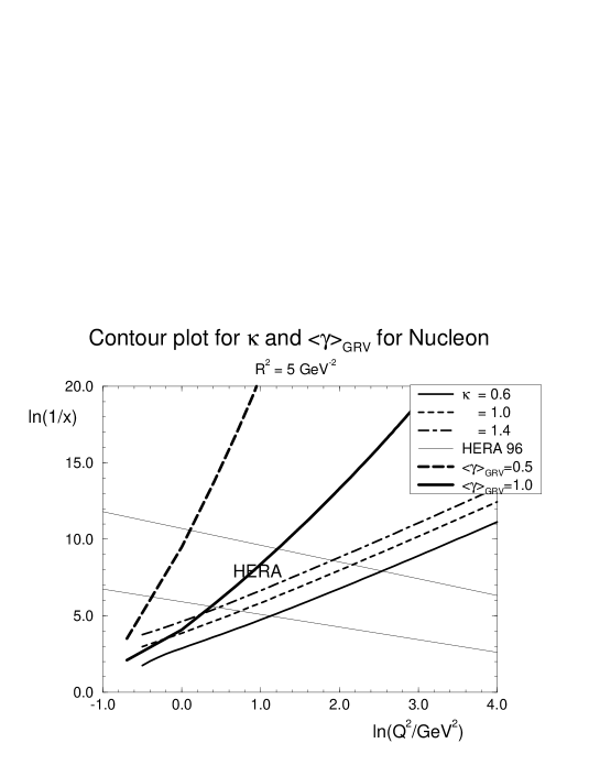
Figure 1: Lines with fixed $<\gamma>$ and $\kappa$ for the GRV parametrization.

A possible answer has been given in two recent papers $\!{}^{{\bf?}}$$\!{}^{{\bf?}}$, in which an attempt has been made to describe the HERA data using the following approach for

$$\gamma^{G}\,=\,\gamma^{\alpha_{S}}\,+\,\gamma^{BFKL}(\frac{N_{c}\alpha_{S}}{\pi\,\omega})\,\,.$$ (12)

In other word, the first row and all terms of the order $(\frac{N_{c}\alpha_{S}}{\pi\,\omega})^{n}$ in the table has been included. Actually, such an approach was suggested long ago in Ref. $\!{}^{{\bf?}}$, where the evolution equation which corresponds to Eq.(12) was written. The main result of these two papers is as follows: using Eq.(12) we can describe all data starting with the flat ($\omega_{0}\,\rightarrow\,0$) initial distribution at $Q^{2}_{0}\,\approx\,1\,GeV^{2}$. Such initial conditions give a natural matching with the “soft” processes. The recent breakthrough in the calculation of the next order correction to the BFKL equation $\!{}^{{\bf?}}$ will lead to calculations in the nearest future of all terms in our table marked by […]. It will allow us to calculate the next correction to Eq.(12) ($\Delta\gamma^{G}$), namely

$$\Delta\gamma^{G}\,=\,\gamma^{\alpha^{2}_{S}}\,+\,\gamma^{\alpha_{S}BFKL}\,=\,\gamma^{\alpha^{2}_{S}}\,+\,\alpha_{S}\,\sum^{\infty}_{n=1}\,(\frac{N_{c}\alpha_{S}}{\pi\,\omega})^{n}\,\,.$$ (13)

Using Eq.(13) we can evaluate the next order corrections and check how well our approach works.

4.3 The second lesson:

The widely held opinion that the DGLAP evolution equations describe the experimental data is too biased. The equations that incorporate the BFKL and DGLAP dynamics lead to better descriptions of the experimental data, providing an excellent matching between the “hard” and “soft” processes - flat initial parton distribution at $Q^{2}\,\approx\,1\,GeV^{2}$.

5 Higher twists

Everything, that has been discussed, so far is related only to the leading twist contribution to the deep inelastic structure function (first term in Eq.(2)). The only way, to separate the leading twist from the higher twist, is to consider sufficiently large value of $Q^{2}$, where the higher twist contribution is expected to be small. However, practical estimates crucially depend on the $Q^{2}$ - dependence of $F^{HT}_{2}$. At first sight it appears that we do not know anything on $F^{HT}_{2}$. Actually, this is not true. We know a lot about the next order twist structure function:

1. The physical meaning $\!{}^{{\bf?}}$, namely,the high twist term is closely related to the correlation function of two partons in the parton cascade.

2.The evolution equations $\!{}^{{\bf?}}$. These equations are similar to the Fadeev equations for many body problem, namely, they reduce the complicated parton interaction to the interaction of two partons with the same kernel as in the original DGLAP equations.

3. The solution of the evolution equation in the region of very small $x$ ( high energy) $\!{}^{{\bf?}}$.

4. This solution suggests the following formula to fit the deep inelastic structure function:

$$F_{2}(x,Q^{2})\,\,=\,\,F^{DGLAP}_{2}(x,Q^{2})\,\,+\,\,\frac{m^{2}}{Q^{2}}c(x)\,[\,F^{DGLAP}_{2}(x,Q^{2})\,]^{2}\,\,,$$

It should be stressed that this expression is quite different from that one which experimentalists assumed, namely, that $F^{HT}_{2}$ has the same $Q^{2}$ and $x$ dependence as $F^{LT}_{2}$.

However, nobody has tried to obtain numerical estimates for the high twist contribution, as the systematic computational approach to the evolution equations for $F^{HT}_{2}$ had not been developed yet.

This has recently been done $\!{}^{{\bf?}}$ and the result is to some extent surprising. The extra power of $Q^{2}$ does not give the feeling that this contribution should be negligibelly small at least at $Q^{2}\,\approx\,10GeV^{2}$. Indeed, if one wants to try a simple parameterization for $F^{HT}_{2}$ it is better to take $F^{HT}_{2}\,\propto\,(F^{LT}_{2})^{2})$ $\!{}^{{\bf?}}$ $\!{}^{{\bf?}}$ and the $Q^{2}$ dependence due to anomalous dimension of $F^{LT}_{2}$ compensates to a large extent for the $1/Q^{2}$ suppression. The importance of this result is obvious, since in all solutions of the DGLAP equations that there are on the market, it has been assumed that the higher twist contribution is small, and can be neglected at $Q^{2}=Q^{2}_{0}$, where $Q^{2}_{0}$ is the initial virtually of the photon from which we start the DGLAP evolution. Notice that in practice the value of $Q^{2}_{0}$ is rather small ( about 4 $GeV^{2}$ ).

5.1 The third lesson:

The common believe that the higher twist contributions are small at $Q^{2}\,\approx\,4\,GeV^{2}$ does not look convincing. We have to study the higher twist contribution in detail as to develop a systematic computational approach to the evolution equations for the higher twist structure function.

6 On the way to complete theory of DIS

6.1 Lattice calculations

For the first time the lattice calculations in DIS has achieved an accuracy that we have to discuss them seriously. We would like to recall, that the lattice experiment gives us solid information on the nonperturbative QCD contribution to DIS. In some sense this is the only way how we can obtain a selfconsistent and reliable nonperturbative contribution.

The experimental errors in the lattice experiments are still large but, nevertheless, it gives a convincing result that the initial quark distributions at $Q^{2}=2.5\,GeV^{2}$ differs from experimental one ( see minireview $\!{}^{{\bf?}}$ at DIS’97). Fig.2 shows the quark distribution predicted by lattice calculation ( see Ref. $\!{}^{{\bf?}}$) and the same distribution that the CTEQ collaboration used as an initial one. Such a difference was expected since in the lattice experiment the leading twist contribution has been calculated while experimental data give the contribution of all twists at a definite value of the virtuality $Q^{2}$. It is interesting to note that the leading twist quark distributions derived on the lattice turn out to be closer to one that was expected in the constituent quark model, where the mean momentum of the quark about $\frac{1}{3}$.

Figure 2: Reconstruction of u-quark distribution from lattice calculation $\!{}^{{\bf?}}$ ( dotted line) and the CTEQ parametrization (solid line) at $\mu^{2}$ = 2.5 $GeV^{2}$.

6.2 The fourth lesson:

The lesson from the first nonperturbative calculation is very simple: our usual method of separation leading twist from the higher twist does not work, the higher twist contribution is still large at $Q^{2}=Q^{2}_{0}\,\approx\,3-4GeV^{2}$.

6.3 A unique opportunity for a theoretical approach to DIS

We would like to emphasize that the lattice calculations give an unique opportunity to develop a self consistent theoretical approach to DIS. The following strategy is advocated . First we use the lattice parton leading twist densities as the initial conditions for the GLAP evolution equations and solve them. The difference between experimental initial parton densities and the lattice one should be treated as the high twist contribution. For them we should use the high twist evolution equations,, and the theoretical status of the higher twist contribution was discussed. The above procedure will provide a theoretical approach to DIS and after it has been achieved we will be able to discuss DIS on the solid theoretical basis. However, the experts in lattice experiments still need to calculate the initial gluon density.

7 Shadowing corrections: miracle or reality?

The HERA data on deep inelastic structure function lead to puzzling result. On one hand, they can be successfully described in the framework of the DGLAP evolution equations without any new ingredients like the BFKL equation and/or the shadowing corrections (SC),as have been discussed above. On the other hand, the parameter ($\kappa$) which gives the estimate for the strength of the SC turns out to be large ($\kappa\,\geq\,1$) in the HERA kinematic region (see Fig.1). This parameter $\kappa$ was estimated in Refs.$\!{}^{{\bf?}}$ $\!{}^{{\bf?}}$ and it is equal to

$$\kappa\,\,=\,\,xG(x,Q^{2})\,\frac{\sigma(GG)}{\pi R^{2}}\,\,=\,\,xG(x,Q^{2})\,\frac{3\pi\alpha_{s}}{Q^{2}\,R^{2}}\,\,.$$ (14)

To understand what is going on, we have to develop a theoretical approach in which we can treat the region of $\kappa\,\approx\,1$ in DIS. It should be stressed that previous attempts to develop a theory for the SC $\!{}^{{\bf?}}$ only had a guaranteed theoretical accuracy for small $\kappa\,\approx\,\alpha_{s}\,\ll\,1$. Two such approaches were discussed recently: in the first one $\!{}^{{\bf?}}$ pQCD was used at the edge of its validity ($\alpha_{s}\kappa\,\leq\,1$), while in the second ( see Refs.$\!{}^{{\bf?}}$ ) the new approach was developed in the kinematic region of high parton density QCD.

In Ref. $\!{}^{{\bf?}}$ a new evolution equation was derived which describes that each parton in the parton cascade interacts with the target in Glauber - Mueller approach $\!{}^{{\bf?}}$. The results are the following: (i) $\kappa$ is the correct parameter that determines the strength of the SC; (ii) the SC to the gluon structure function are big even in the HERA kinematic region, but nevertheless the value of the shadowed gluon structure function is still within the experimental errors or, another way of putting it, the difference between the shadowed and nonshadowed gluon structure functions does not exceed the difference between the gluon structure functions in the different parameterizations such as the MRS,GRV and CTEQ ones; (iii) the SC to $F_{2}(x,Q^{2})$ in HERA kinematic region are so small that they can be neglected; (iv) the SC enter the game before the BFKL equation and, therefore, the BFKL Pomeron cannot be seen in the deep inelastic structure function since it is hidden under substantial SC ( it is interesting to note that this result is seen just from Fig.1 where it is shown that the SC become important in the kinematic region where $<\gamma>$ is still smaller than $\frac{1}{2}$); and (v) in the region of low $x$ the asymptotic behaviour of $xG(x,Q^{2})$ is $xG(x,Q^{2})\,\rightarrow\,\frac{2\,R^{2}\,Q^{2}}{\pi^{2}}\,\ln(1/x)\,\ln\ln(1/x)$. This means that the gluon density is not saturated $\!{}^{{\bf?}}$ unlike for the GLR equation.

The new approach has been developed based on the idea of the semiclassical gluon field in the region of high parton density ( see Refs.$\!{}^{{\bf?}}$,$\!{}^{{\bf?}}$ and $\!{}^{{\bf?}}$ ). The physical problem has been pointed out a long ago ( see Ref. $\!{}^{{\bf?}}$and Ref.$\!{}^{{\bf?}}$ for updated review): at high energy (low $x$ ) and /or for DIS with heavy nucleus we are dealing with the system of partons so dense that conventional methods of pQCD does not work. However, the typical distances are still small for DIS, and this fact results in weak correlations between partons, due to small the coupling constant of QCD.

The revolutionary idea, suggested in Ref. $\!{}^{{\bf?}}$ and developed in Refs. $\!{}^{{\bf?}}$ and $\!{}^{{\bf?}}$, is: in the Bjorken frame for DIS we can replace the complex QCD interaction between parton in such a system by the interaction of a parton $i$ with energy fraction $x_{i}$ with the classical field created by all partons with energy fraction $x$ bigger than $x_{i}$. Indeed, in leading log(1/x) approximation of QCD all parton with $x\,>\,x_{i}$ live for a much longer time than parton $i$, therefore, they create a gluon field which only depends on their density. Using this idea and Wilson renormalization group approach, in Refs.$\!{}^{{\bf?}}$ and $\!{}^{{\bf?}}$ ( see also Ref.$\!{}^{{\bf?}}$ for elucidating remarks), the effective Lagrangian was obtained.

It has been demonstrated that this effective Lagrangian correctly reproduces the DGLAP evolution equations $\!{}^{{\bf?}}$ and even the BFKL Pomeron $\!{}^{{\bf?}}$ in the limit of a sufficiently weak gluon field. However, the main problem in matching the two approaches: one which we discussed above in the beginning of this section and this one, is still an open problem.

8 Crazy ideas

Unfortunately, only two ideas on high energy behaviour of DIS we could call as crazy enough to be interesting.

The first one ( see Ref.$\!{}^{{\bf?}}$ )is a generalization of the renormalization group approach to the longitudinal degrees of freedom. The arguments are based on the $k_{t}$ - factorization $\!{}^{{\bf?}}$ and on similarity between $\ln Q^{2}$ and $\ln s$. The answer is, roughly speaking, the BFKL amplitude, but with running QCD coupling which depends on energy. Certainly, this answer does not contradict unitarity and, perhaps, even the experimental data, but, of course, it is in strong contradiction to the BFKL approach, that has been discussed in section 4. None of the experts have seen a diagram which survives at high energy and in which the running coupling constant depends on $s$, and so it makes the whole approach rather suspicious. On the other hand, this approach is sure to stimulate a more detailed study of this problem.

The second idea is more physical and based on the successful Buchmuller - Haidt parameterization of all data on photon - prpton interaction: photoproduction and DIS $\!{}^{{\bf?}}$. Accordingly to Ref.$\!{}^{{\bf?}}$, the best parameterization of the HERA data is not the solution of the DGLAP evolution equations but a simple formula:

$$F_{2}(x,Q^{2})\,=\,m\,log\frac{(Q^{2}+Q^{2}_{0})}{Q^{2}_{0}}\,\,log\frac{x_{0}}{x}\,\,,$$ (15)

with m = 0.364; $x_{0}$ = 0.04; and $Q^{2}_{0}$ = 0.55 $GeV^{2}$. Eq.(14) gives a correct limit for $F_{2}$ at $Q^{2}\,\rightarrow\,0$ and describes the experimental data on the photoproduction. Such a parameterization leads to the gluon structure function $\!{}^{{\bf?}}$ $xG(x,Q^{2})\,=\,3\,log\frac{x_{0}}{x}$, which energy ( $x$ ) dependence is just the same as the solution to a new evolution equation which takes into account the SC $\!{}^{{\bf?}}$. The physical idea is really crazy and sounds as follows: everything has happened at $x$ of the order of $10^{-2}$, at such values of $x$ the parton densities have reached their asymptotic values and in the region of $x\,\leq\,10^{-2}$ we see only the asymptotic behaviour of the parton densities at low $x$.

9 Resume

I hope that I have convinced you that the low $x$ behaviour of the deep inelastic structure function is still an open problem and the success of the DGLAP evolution equation caused more problems than answers.

I believe, that I gave enough arguments to claim:

1. That corrections to the DGLAP anomalous dimension are not small in HERA kinematic region at low $x$ ;

2. That the higher twist terms are not small at low $x$ even for $Q^{2}\,\approx\,10GeV^{2}$;

3. That the SC are not small in HERA kinematic region.

Therefore, on one hand, we have to add the so called BFKL anomalous dimension to the DGLAP one in the region of small $x$ at HERA, but, on the other hand, the BFKL evolution equation can not be detected due to the background of the strong SC. The explanation of why such different pictures can describe the experimental data, is closely related to the lack of direct measurement of the gluon structure function. Despites the beautiful data on $F_{2}$ at HERA we only know the value of the gluon structure function within 100% errors.

The only way to decide between our theoretical approaches is to predict the behaviour of the other processes at high energy, such as diffractive production, inclusive cross section and correlations in DIS both for nucleon and nuclear targets. Howevere, we have to admit that the accuracy of our theoretical calculations in all other processes, is not as good as for the total cross section of DIS.

The good news is that the success in lattice calculations allows us to a large extent to control the nonperturbative contribution to DIS. Based on the lattice calculation, we can develop a selfconsistent theoretical approach ( see section 6.3) which enable us to clarify some of our problems in near future.

A special chapter of DIS is the “hard” processes with a nuclear target, which I did not touch upon here. They certainly will help us to have a better understanding of both the higher twist contributions and the SC, but this is a subject for a separate talk.

References

References

- [1] K. Wilson: Phys. Rev. 179 (1969) 1444.
- [2] J.C. Collins, D.E. Soper and G. Sterman:Nucl.Phys. B308 (1988) 833.
- [3] V.N. Gribov and L.N. Lipatov:Sov. J. Nucl. Phys. 15 (1972) 438; L.N. Lipatov: Yad. Fiz. 20 (1974) 181; G. Altarelli and G. Parisi:Nucl. Phys. B126 (1977) 298; Yu.L. Dokshitser:Sov. Phys. JETP 46 (1977) 641.
-
[4]
H1 collaboration: S. Aid et al., Nucl. Phys. B470
(1996) 3;
ZEUS collaboration: M. Derrick et al.,Z.Phys. C69 (1996) 607, C72 (1996) 399. - [5] R.G.Roberts:Plenary talk at DIS’97, Chicago, April 1997, RAL-TR-97-024,hep-ph/9706269.
- [6] M. Gluck, E. Reya and A. Vogt: Z.Phys. C67(1995)433.
- [7] A.D. Martin, R.G. Roberts and W.J. Stirling: Phys.Lett.B306(1993)145.
- [8] CTEQ Collaboration, H.L.Lai et al.: Phys.Rev.D51(1995) 4763.
- [9] E.A. Kuraev, L.N. Lipatov and V.S. Fadin: Sov. Phys. JETP 45(1977) 199 ; Ya.Ya. Balitskii and L.V. Lipatov: Sov.J. Nucl. Phys. 28 (1978) 822; L.N. Lipatov: Sov. Phys. JETP 63 (1986) 904.
- [10] L.V. Gribov, E.M. Levin and M.G. Ryskin: Phys. Rep. 100 (1983) 1.
- [11] R.K. Ellis, Z. Kunst and E. M. Levin: Nucl. Phys.B420(1994) 517.
- [12] T. Jaroszewicz:Phys. Lett.B116(1982)291.
- [13] R.S.Thorne: hep - ph /9701241 and references therein.
- [14] J. Kwiecinski, A.D. Martin and A.M. Stasto: hep - ph /9703445.
- [15] V.Fadin: Talk at DIS’97, Chicago, April 1997.
- [16] R.K.Ellis,W. Furmanski and R. Petronzio: Nucl.Phys. B207 (1982)1, B212 (1983) 29.
- [17] A.P. Bukhvostov,G.V. Frolov, L.N. Lipatov and E.A. Kuraev: Nucl. Phys. B258 (1985) 601.
- [18] J. Bartels: Phys. Lett. B298 (1993) 204, Z. Phys. C60 (1993) 471; E.M. Levin, M.G. Ryskin and A.G. Shuvaev: Nucl. Phys. B387 (1992) 589.
- [19] J. Bartels: Talk at DIS’97, Chicago, April 1997.
- [20] G. Schierholz: minireview, Talk at DIS’97, Chicago, April 1997.
- [21] T.Weigl and L. Mankiewicz: Phys. Lett. B339 (1996) 334.
- [22] A.H. Mueller and J. Qiu: Nucl. Phys. B268 (1986) 427.
- [23] A.L. Ayala, M.B. Gay Ducati and E.M. Levin: TAUP 2432 - 97, hep - ph/9706347; Nucl. Phys.B493(1997) 305.
- [24] J. Jalilian-Marian, A. Kovner, L. McLerran and H. Weigert: hep - ph /9606337; H. Weigert: Talk at DIS’97, Chicago, April 1997.
- [25] A.H.Mueller: Nucl. Phys. B335 (1990) 115.
- [26] L. McLerran and R. Venugopalan: Phys. Rev. D49 (1994) 2233,3352, D50 (1994) 2225, D53 (1996) 458.
- [27] J. Jalilian-Marian, A. Kovner, A. Leonidov and H. Weigert: hep - ph/9701284; A. Kovner:Talk at DIS’97, Chicago, April 1997.
- [28] E. Laenen and E. Levin: Ann. Rev. Nucl. Part. 44 (1994) 199.
- [29] Yu.V. Kovchegov: Phys. Rev. D54 (1996) 5463, hep - ph/9701229; Yu.V. Kovchegov, A.H. Mueller and S. Wallon: hep - ph/9704369.
- [30] R.D. Ball and S. Forte:hep-ph/9703417; R.D. Ball: Talk at DIS’97, Chicago, April 1997.
- [31] S.Catani,M. Ciafaloni and F. Hautmann: Phys. Lett. B242 (1990) 97, Nucl. Phys. B366 (1991) 135; J.C. Collins and R.K. Ellis: Nucl. Phys. B360 (1991) 3; E.M. Levin,M.G. Ryskin,Yu.M.Shabelsky and A.G. Shuvaev: Sov.J.Nucl.Phys. 53 (1991) 657.
- [32] W. Buchmueller and D. Haidt: DESY 96-061, D.Haidt: Talk at DIS’97, Chicago, April 1997.