Virtual photon scattering at high energies
as a probe of the short distance pomeron

Abstract

Perturbative QCD predicts the behavior of scattering at high energies and fixed (sufficiently large) transferred momenta in terms of the BFKL pomeron (or short distance pomeron). We study the prospects for testing these predictions in two-photon processes at LEP200 and a possible future $e^{\pm}e^{-}$ collider. We argue that the total cross section for scattering two photons sufficiently far off shell provides a clean probe of BFKL dynamics. The photons act as color dipoles with small transverse size, so that the QCD interactions can be treated perturbatively. We analyze the properties of the QCD result and the possibility of testing them experimentally. We give an estimate of the rates expected and discuss the uncertainties of these results associated with the accuracy of the present theoretical calculations.

I Introduction

The behavior of scattering in the limit of high energy and fixed momentum transfer is described in QCD, at least for situations in which perturbation theory applies, by the Balitskii-Fadin-Kuraev-Lipatov (BFKL) pomeron [1] (or short distance pomeron). Attempts to test experimentally this sector of QCD have started in the last few years, mainly based on measurements of deeply inelastic events at low values of the Bjorken variable $x$ in lepton-hadron scattering [2] and jet production at large rapidity separations in hadron-hadron collisions [3]. In this paper we study the possibilities for investigating QCD pomeron effects in a different context, namely in photon-photon scattering at $e^{+}\,e^{-}$ colliders, where the photons are produced from the lepton beams by bremsstrahlung. The results of this paper also apply to $e^{-}\,e^{-}$ or $\mu^{\pm}\,\mu^{-}$ colliders. Some aspects of this study have been presented in Refs. [4, 5, 6].

The quantity we consider is the total cross section for off-shell photon scattering at high energy. This can be measured in $e^{+}\,e^{-}$ collisions in which both the outgoing leptons are tagged. This cross section presents some theoretical advantages as a probe of QCD pomeron dynamics compared to the structure functions for deeply inelastic scattering off a proton (see for instance the discussion in Ref. [2]) or a (quasi)-real photon (see for example Ref. [7]), essentially because it does not involve a non-perturbative target. Unlike protons or quasi-real photons, virtual photon states can be described through perturbative wave functions. In some respects the off-shell photon cross section presents analogies with the process of scattering of two quarkonia (or “onia”), which has been proposed as a gedanken experiment to investigate the high energy regime in QCD [8]. In this case, non-perturbative effects are suppressed by the smallness of the onium radius. In the case of virtual photons the size of the wave function is controlled by the photon virtuality instead of the heavy quark mass. It is an interesting feature of investigations at $e^{+}e^{-}$ colliders that this size can be tuned by measuring the momenta of the outgoing leptons.

On the other hand, such experimental studies may prove to be difficult due to the smallness of the available rates. As we shall see, for large photon virtualities $Q^{2}$ the cross section falls off like $1/Q^{2}$. An estimate of the number of events that one may expect to be available for such studies at LEP200 and a future linear $e^{+}e^{-}$ collider will be provided later in the paper.

There have recently been other investigations of the high energy regime in the context of photon-photon scattering. Balitskii [9] has proposed an expansion of the scattering amplitude in the high energy limit in terms of Wilson line operators. This method provides an elegant reformulation of the BFKL problem, and may prove to be useful to get beyond the leading logarithm approximation. Bartels, De Roeck and Lotter [10] have evaluated the photon-photon cross section at present and future $e^{+}e^{-}$ colliders. Their results are similar to those in Refs. [4, 5, 6]. In Ref. [7] detailed studies have been carried out for diffractive meson production and photon structure functions at LEP200.

To describe the electron-positron scattering process (Fig. 1), we will parametrize the five-fold differential cross section as

$${{d\,\sigma^{(e^{+}e^{-})}}\over{dx_{A}\,dx_{B}\,dQ^{2}_{A}\,dQ^{2}_{B}\,d\phi/(2\,\pi)}}={{d\,\sigma^{(e^{+}e^{-})}}\over{dx_{A}\,dx_{B}\,dQ^{2}_{A}\,dQ^{2}_{B}}}\,\left[1+A_{1}\,\cos{\phi}+A_{2}\,(2\,\cos^{2}{\phi}-1)\right]\hskip 22.76228pt.$$ (1)

Here we denote by $x_{A},\,x_{B}$ the fractions of the longitudinal momenta of the leptons A and B that are carried by the photons, by $Q_{A}^{2}=-q_{A}^{\mu}q_{A\,\mu},\,Q_{B}^{2}=-q_{B}^{\mu}q_{B\,\mu}$ the photon virtualities, and by $\phi$ the angle between the lepton scattering planes in a frame in which the photons are aligned with the $z$ axis. The overall factor in the right hand side gives the distribution averaged over the angle $\phi$, while $A_{1}$, $A_{2}$ are the asymmetries.

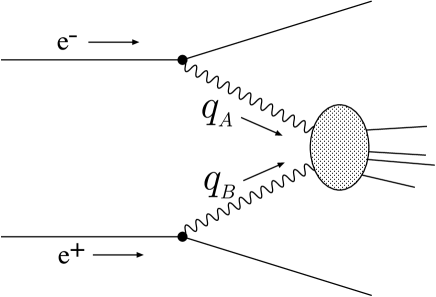
FIG. 1.: The photon-photon scattering process in $e^{+}e^{-}$ collisions.

We will start by considering the $\phi$-averaged cross section, and we will express it in the equivalent photon approximation [11] by folding the $\gamma^{*}\,\gamma^{*}$ cross section with the flux of photons from each lepton. This flux is proportional to the probability density for the splitting $e\to e\,\gamma$, and depends on the photon polarization. We will thus write

$${{Q^{2}_{A}\,Q^{2}_{B}\,d\,\sigma^{(e^{+}e^{-})}}\over{dx_{A}\,dx_{B}\,dQ^{2}_{A}\,dQ^{2}_{B}}} = \left({\alpha\over{2\,\pi}}\right)^{2}\left\{P_{\gamma/e^{+}}^{(T)}(x_{A})\,P_{\gamma/e^{-}}^{(T)}(x_{B})\,\sigma_{{\gamma^{*}}{\gamma^{*}}}^{(TT)}(x_{A}\,x_{B}\,s,Q_{A}^{2},Q_{B}^{2})\right.$$ (5)

$$+P_{\gamma/e^{+}}^{(T)}(x_{A})\,P_{\gamma/e^{-}}^{(L)}(x_{B})\,\sigma_{{\gamma^{*}}{\gamma^{*}}}^{(TL)}(x_{A}\,x_{B}\,s,Q_{A}^{2},Q_{B}^{2})$$

$$+P_{\gamma/e^{+}}^{(L)}(x_{A})\,P_{\gamma/e^{-}}^{(T)}(x_{B})\,\sigma_{{\gamma^{*}}{\gamma^{*}}}^{(LT)}(x_{A}\,x_{B}\,s,Q_{A}^{2},Q_{B}^{2})$$

$$+\left.P_{\gamma/e^{+}}^{(L)}(x_{A})\,P_{\gamma/e^{-}}^{(L)}(x_{B})\,\sigma_{{\gamma^{*}}{\gamma^{*}}}^{(LL)}(x_{A}\,x_{B}\,s,Q_{A}^{2},Q_{B}^{2})\right\}\,\;\;\;,$$

where the transverse and longitudinal photon flux factors $P^{(T)}$, $P^{(L)}$ are given by

$$P_{\gamma/e}^{(T)}(x)={{1+(1-x)^{2}}\over x}\hskip 17.07182pt,\hskip 22.76228ptP_{\gamma/e}^{(L)}(x)=2\,{{1-x}\over x}\hskip 22.76228pt,$$ (6)

and $\sigma_{{\gamma^{*}}{\gamma^{*}}}^{(a\,b)}$, with $a,b=T,L$, is the cross section for the scattering of two photons with polarizations $a$ and $b$.

We will proceed in the following way. In Sec. II we set our notations and describe the Born approximation to the photon-photon cross section at high energy. In this section we concentrate on the case of transversely polarized photons, that is, the cross section $\sigma_{{\gamma^{*}}{\gamma^{*}}}^{(TT)}$ in Eq. (5) above. In Sec. III we extend these results to include the full polarization dependence and we discuss the associated asymmetries. In Sec. IV we consider the summation of the leading logarithmic corrections to the photon-photon cross section due to BFKL pomeron exchange, and emphasize how the perturbative results depend on the total energy and the photon virtualities. Secs. V and VI are devoted to discussing some of the limitations of the treatment based on the BFKL equation. In Sec. V we focus on the dependence of the cross section on two mass scales (in the running coupling and in the high energy logarithms), which are left undetermined in a leading log analysis. In Sec. VI we consider the limitations of using the BFKL approach that follow from the behavior at very large $s$. Sec. VII illustrates how to relate the summed result for the photon-photon cross section to the small-$x$ behavior of the photon deeply inelastic structure function. In Sec. VIII we compare the QCD result with expectations based on traditional Regge theory. In Sec. IX we consider the limit of low photon virtualities and discuss the region of transition between hard and soft scattering. The rates at the level of the $e^{+}e^{-}$ cross section are examined in Sec. X. Some concluding remarks are given in Sec. XI. We collect in Appendix A the details of the Born order calculation, and in Appendix B some formulas which are useful for comparing the gluon-exchange and quark-exchange contributions to the photon-photon cross section.

II Notations and lowest order calculation

We consider the total cross section for the scattering of two transversely polarized virtual (space-like) photons $\gamma^{*}(q_{A})$ and $\;\gamma^{*}(q_{B})$, with virtualities $q_{A}^{2}\equiv-Q^{2}_{A}$ and $q_{B}^{2}\equiv-Q^{2}_{B}$, in the high energy region where the center-of-mass energy $\sqrt{s}\equiv\sqrt{(q_{A}+q_{B})^{2}}$ is much larger than $Q_{A}$, $Q_{B}$. We also suppose that the photon virtualities are in turn large with respect to the QCD scale $\Lambda_{QCD}^{2}$, so that the process occurs at short distances (much smaller than $\Lambda^{-1}_{QCD}\approx 1\;{\mbox{fm}}$) and QCD perturbation theory applies.

We work in a reference frame in which the incoming photons have zero transverse momenta, and are boosted along the positive and negative light-cone directions. For a four-momentum $p^{\mu}$, we define the “$+$” and “$-$” momentum components $p^{+}$, $p^{-}$ as

$$p^{\pm}=\left(p^{0}\pm p^{3}\right)/\sqrt{2}\;\;\;.$$ (7)

The incoming photon momenta are parametrized as follows in a notation where $q^{\mu}=(q^{+},q^{-},{\bf q}_{T})$:

$$q^{\mu}_{A}=\left(q^{+}_{A},-{Q_{A}^{2}\over{2\;q^{+}_{A}}},{\mbox{\bf 0}}\right)\;\;,\;\;\;q^{\mu}_{B}=\left(-{Q_{B}^{2}\over{2\;q^{-}_{B}}},q^{-}_{B},{\mbox{\bf 0}}\right)\;\;.$$ (8)

Here the “$+$” and “$-$” components $q^{+}_{A},q^{-}_{B}$ approximately build up the total energy $s$, and are much larger than the initial virtualities

$$2\,q^{+}_{A}\,q^{-}_{B}\approx s\gg Q_{A}^{2},Q_{B}^{2}\;\;\;.$$ (9)

The Born contribution to this cross section is given by the high energy approximation to the reaction

$$\gamma^{*}(q_{A})+\gamma^{*}(q_{B})\to q(p_{A})+{\bar{q}}({\bar{p}}_{A})+q(p_{B})+{\bar{q}}({\bar{p}}_{B})\;\;\;$$ (10)

in lowest order perturbation theory. The corresponding diagrams involve the exchange of two gluons between the two quark-antiquark pairs [12], and are exemplified in Fig. 2.

We parametrize the outgoing quark momenta as

$$p^{\mu}_{A}=\left(z_{A}q^{+}_{A},z_{A}^{\prime}q^{-}_{B},{{\bf p}}_{A}\right)\;\;,\;\;\;p^{\mu}_{B}=\left(z_{B}^{\prime}q^{+}_{A},z_{B}q^{-}_{B},{{\bf p}}_{B}\right)\;\;,$$ (11)

and denote by $k^{\mu}$ the exchanged gluon momentum.

In the high energy limit defined by Eq. (9), the kinematic region which dominates the integrations is the one in which the transverse momenta flowing in the loops are of the order of the initial virtualities, and the light-cone components of the exchanged gluon are suppressed with respect to the transverse momenta by a quantity of order $Q_{A}/\sqrt{s}$ or $Q_{B}/\sqrt{s}$, so that $k^{2}\simeq-{{\bf k}}^{2}$.

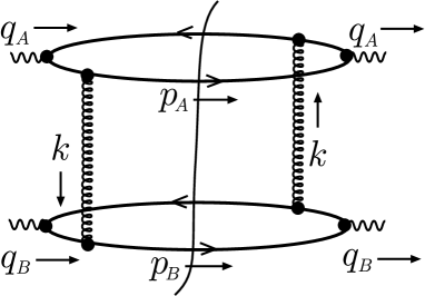
FIG. 2.: One of the two-gluon exchange graphs contributing to the high energy $\gamma^{*}\gamma^{*}$ cross section in the Born approximation. The gluons can be attached to the quark lines in $2^{4}$ different ways.

The squared amplitude for the graph in Fig. 2, integrated over the final quark and antiquark phase space, for fixed transverse photon polarizations $\varepsilon_{A}$, $\varepsilon_{B}$, is given by

$${|{\cal M}|}^{2}=\int\;{{d^{4}\,k}\over{(2\,\pi)^{4}}}\;{{d^{4}\,p_{A}}\over{(2\,\pi)^{4}}}\;{{d^{4}\,p_{B}}\over{(2\,\pi)^{4}}}\;{1\over{(k^{2})^{2}}}\;2\,\pi\,\delta_{+}\!\left(p_{A}^{2}\right)\,\;2\,\pi\,\delta_{+}\!\left(p_{B}^{2}\right)\,\sum_{a,b}\,$$ (12)

$$\times\,\;2\,\pi\,\delta_{+}\!\left((q_{A}-p_{A}-k)^{2}\right)\,\;2\,\pi\,\delta_{+}\!\left((q_{B}-p_{B}+k)^{2}\right)\,\,$$ (13)

$$\times\,{{{\rm Tr}\Bigl{[}{\hbox to0.0pt{/\hss}p}_{A}\,(i\,g_{s}t^{r}\gamma_{\alpha})\,i\,({\hbox to0.0pt{/\hss}p}_{A}+\hbox to0.0pt{/\hss}k)(i\,e_{a}\,e\,{\hbox to0.0pt{/\hss}\varepsilon}_{A})({\hbox to0.0pt{/\hss}q}_{A}-{\hbox to0.0pt{/\hss}p}_{A}-\hbox to0.0pt{/\hss}k)(-i\,g_{s}t^{s}\gamma_{\beta})(-i)({\hbox to0.0pt{/\hss}p}_{A}-{\hbox to0.0pt{/\hss}q}_{A})(-i\,e_{a}\,e\,{\hbox to0.0pt{/\hss}\varepsilon}_{A})\Bigr{]}}\over{\left((p_{A}+k)^{2}+i\,\varepsilon\right)\left((p_{A}-q_{A})^{2}-i\,\varepsilon\right)}}\,\,$$ (14)

$$\times\,{{{\rm Tr}\Bigl{[}{\hbox to0.0pt{/\hss}p}_{B}(ig_{s}t^{r}\gamma^{\alpha})\,i\,({\hbox to0.0pt{/\hss}p}_{B}-\hbox to0.0pt{/\hss}k)\,(i\,e_{b}\,e{\hbox to0.0pt{/\hss}\varepsilon}_{B})\,({\hbox to0.0pt{/\hss}q}_{B}-{\hbox to0.0pt{/\hss}p}_{B}+\hbox to0.0pt{/\hss}k)(-ig_{s}t^{s}\gamma^{\beta})(-i)({\hbox to0.0pt{/\hss}p}_{B}-{\hbox to0.0pt{/\hss}q}_{B})(-ie_{b}e{\hbox to0.0pt{/\hss}\varepsilon}_{B})\Bigr{]}}\over{\left((p_{B}-k)^{2}+i\,\varepsilon\right)\left((p_{B}-q_{B})^{2}-i\,\varepsilon\right)}}\;\;.$$ (15)

Here $e_{a}$, $e_{b}$ are the electric charges of the quarks in units of $e=\sqrt{4\,\pi\,\alpha}$, and the indices $a,b$ run over the light quark flavors, $u,d,s$. (The flavors $c,b$ need a separate treatment.) In the high energy approximation this amplitude takes the form

$${|{\cal M}|}^{2}=32\,\alpha^{2}\,\alpha_{s}^{2}\,\left(\sum_{q}e^{2}_{q}\right)^{2}\,(2\,\pi)^{2}\,(2\,s)\,\int\;{{d^{2}\,{\bf k}}\over{(2\,\pi)^{2}}}\;{{d^{2}\,{{\bf p}}_{A}}\over{(2\,\pi)^{2}}}\;{{d^{2}\,{{\bf p}}_{B}}\over{(2\,\pi)^{2}}}\;\int_{0}^{1}{d\,z_{A}}\int_{0}^{1}{d\,z_{B}}\,{1\over{({{\bf k}}^{2})^{2}}}\,$$ (16)

$$\times\,{{\left[4z_{A}(1-z_{A}){\bf{\varepsilon}}_{A}\cdot{{\bf p}}_{A}\;{\bf{\varepsilon}}_{A}\cdot({{\bf p}}_{A}+{\bf k})-{{\bf p}}_{A}\cdot({{\bf p}}_{A}+{\bf k})\right]}\over{\left[z_{A}\,(1-z_{A})\,Q^{2}_{A}+({{\bf p}}_{A}+{{\bf k}})^{2}\right]\,\left[z_{A}\,(1-z_{A})\,Q^{2}_{A}+{{\bf p}}_{A}^{2}\right]\,}}\,$$ (17)

$$\times\,{{\left[4z_{B}(1-z_{B}){\bf{\varepsilon}}_{B}\cdot{{\bf p}}_{B}\;{\bf{\varepsilon}}_{B}\cdot({{\bf p}}_{B}-{\bf k})-{{\bf p}}_{B}\cdot({{\bf p}}_{B}-{\bf k})\right]}\over{\left[z_{B}\,(1-z_{B})\,Q^{2}_{B}+({{\bf p}}_{B}-{{\bf k}})^{2}\right]\,\left[z_{B}\,(1-z_{B})\,Q^{2}_{B}+{{\bf p}}_{B}^{2}\right]\,}}\;\;\;\;\;\;\;\;.$$ (18)

See Appendix A for details of this calculation.

The amplitudes for the other graphs, in which the gluons are connected to different fermion lines, can be derived from Eq. (16) by using the replacements

$$\left[z_{A}\,(1-z_{A})\,Q^{2}_{A}+({{\bf p}}_{A}+{{\bf k}})^{2}\right]\to{{1-z_{A}}\over{z_{A}}}\,\left[z_{A}\,(1-z_{A})\,Q^{2}_{A}+{{\bf p}}_{A}^{2}\right]\,$$ (19)

in the denominator, and

$$({{\bf p}}_{A}+{{\bf k}})\to-{{1-z_{A}}\over{z_{A}}}\,{{\bf p}}_{A}\,$$ (20)

in the numerator. (Analogous replacements hold for the momentum components of the quark $p_{B}$). In addition, the contribution from the graphs in which the quark and antiquark lines are interchanged can be obtained by symmetrizing the above expressions with respect to ${{\bf p}}_{A}\to{{\bf p}}_{A}+{{\bf k}}$ (and, analogously, ${{\bf p}}_{B}\to{{\bf p}}_{B}-{{\bf k}}$).

We add the graphs, and divide by $2\,s$ to form the $\gamma^{*}\,\gamma^{*}$ cross section

$$\sigma^{(0)}_{{\gamma^{*}}{\gamma^{*}}}={1\over{2\,s}}\,{|{\cal M}|}^{2}\;\;\;\;.$$ (21)

We find

$$\sigma^{(0)}_{{\gamma^{*}}{\gamma^{*}}}(s,Q_{A}^{2},Q_{B}^{2},{\bf{\varepsilon}}_{A},{\bf{\varepsilon}}_{B})={1\over{2\,\pi}}\,\int\,{{d^{2}\,{\bf k}}\over{\pi}}\,{1\over{({{\bf k}}^{2})^{2}}}\,G({\bf k};Q^{2}_{A},{\bf{\varepsilon}}_{A})\,G(-{\bf k};Q^{2}_{B},{\bf{\varepsilon}}_{B})\;\;\;\;.$$ (22)

The factors $1/\left({{\bf k}}^{2}\right)^{2}$ in this formula come from the gluon propagators. These factors multiply functions $G({\bf k};Q^{2},{\bf{\varepsilon}})$, which describe the coupling of the exchanged gluon to the quark-antiquark system created by the virtual photon with virtuality $Q^{2}$ and transverse polarization ${\bf{\varepsilon}}$. The explicit expression for $G$ is

$$G({\bf k};Q^{2},{\bf{\varepsilon}})=4\,\alpha\,\alpha_{s}\,\left(\sum_{q}e^{2}_{q}\right)\,\int\;{{d^{2}\,{{\bf p}}}\over{\pi}}\;\int_{0}^{1}\,{d\,z}\,$$ (23)

$$\times\,\left\{{{\left[{{\bf p}}^{2}-4z(1-z)({\bf{\varepsilon}}\cdot{{\bf p}})^{2}\;\right]}\over{\left[{{\bf p}}^{2}+z\,(1-z)\,Q^{2}\right]^{2}}}-{{\left[{{\bf p}}\cdot({{\bf p}}+{\bf k})-4z(1-z){\bf{\varepsilon}}\cdot{{\bf p}}\;{\bf{\varepsilon}}\cdot({{\bf p}}+{\bf k})\right]}\over{\left[({{\bf p}}+{{\bf k}})^{2}+z\,(1-z)\,Q^{2}\right]\,\left[{{\bf p}}^{2}+z\,(1-z)\,Q^{2}\right]}}\right\}\;\;\;\;.$$ (24)

The functions $G$ can be thought of as “color functions” of the virtual photon since they describe the color flow in the $q\bar{q}$ states. From the point of view of light-cone perturbation theory [13], they correspond to the coupling of the null-plane photon wave function to gluons.

In the remainder of this section we discuss the case of the average over the two transverse photon polarizations. The detailed polarization dependence of the color functions $G$ and the associated polarization asymmetry in the cross section are treated in Sec. III. By taking the polarization average

$${1\over 2}\,\sum_{\lambda}{\bf{\varepsilon}}_{i}^{(\lambda)}{\bf{\varepsilon}}_{j}^{(\lambda)}\to{1\over 2}\,\delta_{\,i\,j\,}\hskip 17.07182pt,\\$$ (25)

we define the function $G_{1}$

$$G_{1}({{\bf k}}^{2}/Q^{2})={1\over 2}\,\sum_{\lambda}G({\bf k};Q^{2},{\bf{\varepsilon}}^{(\lambda)})\hskip 17.07182pt.$$ (26)

We find

$$G_{1}({{\bf k}}^{2}/Q^{2})=4\,\alpha\,\alpha_{s}\,\left(\sum_{q}e^{2}_{q}\right)\,\int\;{{d^{2}\,{{\bf p}}}\over{\pi}}\;\int_{0}^{1}\,{d\,z}\left[z^{2}+(1-z)^{2}\right]\,$$ (27)

$$\times\,\left[{{{{\bf p}}^{2}}\over{\left[{{\bf p}}^{2}+z\,(1-z)\,Q^{2}\right]^{2}}}-{{{{\bf p}}\cdot({{\bf p}}+{\bf k})}\over{\left[({{\bf p}}+{{\bf k}})^{2}+z\,(1-z)\,Q^{2}\right]\,\left[{{\bf p}}^{2}+z\,(1-z)\,Q^{2}\right]}}\right]\;\;.$$ (28)

Each one of the two ${{\bf p}}$-dependent terms in the integrand of Eq. (27) would lead to an ultraviolet divergent integral, but the divergence cancels in the sum, illustrating that the gluon does not couple to the color singlet $q{\bar{q}}$ system in the limit ${{\bf p}}^{2}\to\infty$. The photon virtuality $Q^{2}$ regularizes the denominators in the infrared region, ${{\bf p}}^{2}\to 0$. In the limit of small $Q^{2}$, the probability density $P_{q/\gamma}(z)=\left[z^{2}+(1-z)^{2}\right]/2$ for the splitting of a transversely polarized photon into a quark-antiquark pair $(\gamma\to q{\bar{q}})$ correctly factors out in front of the logarithmic singularity $d{{\bf p}}^{2}/{{\bf p}}^{2}$ associated with the region of strong ordering $Q^{2}\ll{{\bf p}}^{2}\ll{{\bf k}}^{2}$.

By introducing the Feynman parametrization

$${1\over{\left[({{\bf p}}+{{\bf k}})^{2}+z\,(1-z)\,Q^{2}\right]\,\left[{{\bf p}}^{2}+z\,(1-z)\,Q^{2}\right]^{2}}}$$ (29)

$$\hskip 56.9055pt\,=\int^{1}_{0}\,d\lambda\,{{2\,(1-\lambda)}\over{\left[({{\bf p}}+\lambda\,{{\bf k}})^{2}+z\,(1-z)\,Q^{2}+\lambda\,(1-\lambda){{\bf k}}^{2}\right]^{3}}}$$ (30)

and carrying out the integration over the shifted transverse momentum variable ${{\bf p}}^{\prime}={{\bf p}}+\lambda\,{{\bf k}}$ in Eq. (27), one can obtain the following useful representation of the function $G_{1}({{\bf k}}^{2}/Q^{2})$ as an integral over two dimensionless variables:

$$G_{1}({{\bf k}}^{2}/Q^{2})=2\,\alpha\,\alpha_{s}\,\left(\sum_{q}e^{2}_{q}\right)\,{{\bf k}}^{2}\,\int_{0}^{1}\,{d\,z}\,\int_{0}^{1}\,{d\,\lambda}\,{{\left[\lambda^{2}+(1-\lambda)^{2}\right]\,\left[z^{2}+(1-z)^{2}\right]}\over{\lambda\,(1-\lambda)\,{{\bf k}}^{2}+z\,(1-z)\,Q^{2}}}\hskip 14.22636pt.$$ (31)

This representation explicitly shows that the distribution $\left({{\bf k}}^{2}\right)^{-1}G_{1}({{\bf k}}^{2}/Q^{2})$ is symmetric under interchange of the space-like boson virtualities ${{\bf k}}^{2}$ and $Q^{2}$. In the configurations in which one of the virtualities is much smaller than the other one, this distribution is logarithmically enhanced. More precisely, we find

$${1\over{{{\bf k}}^{2}}}\,G_{1}({{{{\bf k}}^{2}}/{Q^{2}}})\sim 4\,\alpha\,\alpha_{s}\,\left(\sum_{q}e^{2}_{q}\right)\;{2\over 3}\,{1\over{Q^{2}}}\,\left[\ln{{Q^{2}}\over{{{\bf k}}^{2}}}+{\cal O}\left(1\right)\right]\hskip 14.22636pt,\hskip 22.76228pt{{\bf k}}^{2}\ll Q^{2}\hskip 14.22636pt,$$ (32)

$${1\over{{{\bf k}}^{2}}}\,G_{1}({{{{\bf k}}^{2}}/{Q^{2}}})\sim 4\,\alpha\,\alpha_{s}\,\left(\sum_{q}e^{2}_{q}\right)\;{2\over 3}\,{1\over{{{\bf k}}^{2}}}\,\left[\ln{{{{\bf k}}^{2}}\over{Q^{2}}}+{\cal O}\left(1\right)\right]\hskip 14.22636pt,\hskip 22.76228pt{{\bf k}}^{2}\gg Q^{2}\hskip 14.22636pt,$$ (33)

where the coefficient in front of the logarithm is given by the first moment of the splitting density

$$\int_{0}^{1}\,{d\,x}\left[x^{2}+(1-x)^{2}\right]={2\over 3}\hskip 28.45274pt.$$ (34)

The logarithmic behavior at small ${{\bf k}}^{2}$ comes from the region ${{\bf k}}^{2}\ll{{\bf p}}^{2}\ll Q^{2}$. Here the quark transverse momentum is much smaller than the photon virtuality, and the quark longitudinal momentum fraction is very small, $z\ll 1$ (or $(1-z)\ll 1$). This region is sometimes referred to as the aligned-jet region, and corresponds to configurations in which the $q{\bar{q}}$ system fluctuates to large sizes [14]. Note that while for the case at hand of the $\gamma^{*}\,\gamma^{*}$ total cross section this region contributes only a logarithmic enhancement, for the case of non-inclusive processes, such as processes involving rapidity gaps, this is expected to become the dominant contribution [15].

The integration over the parameter $\lambda$ in Eq. (31) can be explicitly performed. This yields

$$G_{1}(\eta)=2\,\alpha\,\alpha_{s}\,\left(\sum_{q}e^{2}_{q}\right)\,\int_{0}^{1}\,{{d\,\xi}\over{\sqrt{1-\xi}}}\,\left(1-{\xi\over 2}\right)\,\left[{{\eta+{\xi/2}}\over{\sqrt{\eta\,(\eta+\xi)}}}\,\ln{\left({{\sqrt{\eta+\xi}+\sqrt{\eta}}\over{\sqrt{\eta+\xi}-\sqrt{\eta}}}\right)}-1\right]\,,$$ (35)

where we have introduced the variables

$$\xi\equiv 4\,z\,(1-z)\hskip 28.45274pt,\hskip 56.9055pt\eta\equiv{{\bf k}}^{2}/Q^{2}\hskip 28.45274pt.$$ (36)

In Fig. 3, we report the result of the numerical evaluation of the integral (35) by plotting the function $G_{1}$ versus $\eta={{\bf k}}^{2}/Q^{2}$.

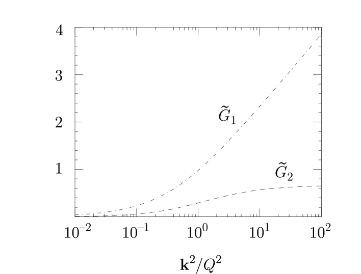
FIG. 3.: The ${{\bf k}}^{2}/Q^{2}$ dependence of the color functions $G_{1}$ (see Sec. II) and $G_{2}$ (see Sec. III). We plot the normalized functions ${\tilde{G}}=G/(4\,\alpha\,\alpha_{s}\,\sum_{q}e^{2}_{q})$.

The unpolarized $\gamma^{*}\,\gamma^{*}$ cross section to Born order, ${\overline{\sigma}}^{(0)}$, can be obtained by inserting the result for the function $G_{1}$ in the general formula (22). It is convenient to use the representation (31) of $G_{1}$. By substituting this representation in Eq. (22), and carrying out the integration over the gluon transverse momentum ${{\bf k}}$, we obtain

$${\overline{\sigma}}^{(0)}(s,Q_{A}^{2},Q_{B}^{2})={{2\,\alpha^{2}\,\alpha_{s}^{2}\,\left(\sum_{q}e^{2}_{q}\right)^{2}}\over{\pi}}\,\int_{0}^{1}\,{d\,z_{A}}\left[z_{A}^{2}+(1-z_{A})^{2}\right]\int_{0}^{1}\,{d\,\lambda_{A}}\left[\lambda_{A}^{2}+(1-\lambda_{A})^{2}\right]\,$$ (37)

$$\times\int_{0}^{1}\,{d\,z_{B}}\left[z_{B}^{2}+(1-z_{B})^{2}\right]\int_{0}^{1}\,{d\,\lambda_{B}}\left[\lambda_{B}^{2}+(1-\lambda_{B})^{2}\right]\,$$ (38)

$$\times{{\ln\left[{Q_{A}^{2}\,z_{A}\,(1-z_{A})\,\lambda_{B}\,(1-\lambda_{B})}/\left({Q_{B}^{2}\,z_{B}\,(1-z_{B})\,\lambda_{A}\,(1-\lambda_{A})}\right)\right]}\over{Q_{A}^{2}\,z_{A}\,(1-z_{A})\,\lambda_{B}\,(1-\lambda_{B})-Q_{B}^{2}\,z_{B}\,(1-z_{B})\,\lambda_{A}\,(1-\lambda_{A})}}\hskip 14.22636pt.$$ (39)

This formula provides an expression for the cross section in the large $s$ limit in terms of dimensionless integrals, which allows us to study the dependence on the energy and mass scales. To this order in perturbation theory the cross section has a constant behavior with the energy $s$. The cross section depends on the mass scales $Q_{A}^{2}$ and $Q_{B}^{2}$ only. Factoring out an overall scale factor $1/(Q_{A}\,Q_{B})$ in Eq. (37), we are left with a function $\tilde{\sigma}(r)$ of the ratio $r\equiv Q_{A}/Q_{B}$:

$$\bar{\sigma}^{(0)}=16\alpha^{2}\alpha_{s}^{2}\left({\sum_{q}e_{q}^{2}}\right)^{2}{\tilde{\sigma}(r)\over Q_{A}Q_{B}}.$$ (40)

The function $\tilde{\sigma}(r)$ can be computed by performing numerically the integrations over the dimensionless variables $z$’s and $\lambda$’s. The result is plotted in Fig. 4.

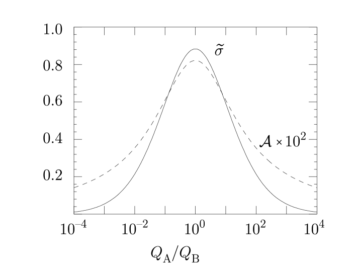
FIG. 4.: The high-energy $\gamma^{*}\gamma^{*}$ cross section in the Born approximation as a function of the ratio $r\equiv Q_{A}/Q_{B}$ between the photon virtualities. The solid line is the rescaled cross section $\tilde{\sigma}(r)$ defined in Eq. (40). The dashed line is the polarization asymmetry discussed in Sec. III (see Eq. (57)), multiplied by $10^{2}$.

Notice that the dependence of $\tilde{\sigma}(r)$ on $r$ is rather mild when $r$ is near 1. Thus, in this region, $\tilde{\sigma}(r)$ in Eq. (40) could be treated as a constant, so that

$${\overline{\sigma}}^{(0)}\sim 1/\left(Q_{A}\,Q_{B}\right)\hskip 14.22636pt,\hskip 22.76228ptr\approx 1\hskip 14.22636pt.$$ (41)

When, in contrast, the two virtualities are widely disparate from each other, either $r\gg 1$ or $r\ll 1$, the function $\tilde{\sigma}(r)$ has a strong dependence on $r$, vanishing linearly (modulo logarithmic enhancements) with either $r^{-1}$ or $r$, respectively. This provides the overall change of scale in the cross section

$${\overline{\sigma}}^{(0)}\sim 1/Q_{A}^{2}\hskip 14.22636pt,\hskip 22.76228ptQ_{A}^{2}\gg Q_{B}^{2}\hskip 14.22636pt,$$ (42)

$${\overline{\sigma}}^{(0)}\sim 1/Q_{B}^{2}\hskip 14.22636pt,\hskip 22.76228ptQ_{B}^{2}\gg Q_{A}^{2}\hskip 14.22636pt.$$ (43)

We will come back to this later on and examine the details of these behaviors numerically (see Sec. VII).

III Polarization dependence

We now study the dependence of the color functions $G$ and of the photon-photon cross section on the polarization of the virtual photon. Working in the frame defined by Eq. (8), and denoting by $u$, $v$ the lightlike unit vectors

$$u=\left(1,0,{\mbox{\bf 0}}\right)\;\;,\;\;\;v=\left(0,1,{\mbox{\bf 0}}\right)\;\;,$$ (44)

we introduce the following decomposition of the polarization tensor for the photon $q_{A}$:

$$-g_{\mu\nu}=\sum_{i=1,2}\varepsilon_{\mu}^{i}(q_{A})\varepsilon_{\nu}^{i}(q_{A})-{{Q_{A}^{2}}\over{(q_{A}\cdot v)^{2}}}v_{\mu}\,v_{\nu}-{{{q_{A}}_{\mu}\,v_{\nu}+v_{\mu}\,{q_{A}}_{\nu}}\over{q_{A}\cdot v}}\;\;.$$ (45)

The index $i$ in the first term in the right hand side of Eq. (45) runs over the transverse polarizations. We describe these polarizations by using the linear basis

$$\varepsilon_{\mu}^{i}(q_{A})=\delta_{\mu}^{i}\hskip 17.07182pt,\hskip 5.69046pti=1,2\hskip 17.07182pt.$$ (46)

From the second term in the right hand side of Eq. (45), we define the longitudinal polarization vector as

$$\varepsilon_{\mu}^{L}(q_{A})={{Q_{A}}\over{q_{A}\cdot v}}v_{\mu}\;\;.$$ (47)

The last term in Eq. (45) does not contribute because of current conservation. We thus have

$$-g_{\mu\nu}=\sum_{i=1,2}\varepsilon_{\mu}^{i}(q_{A})\,\varepsilon_{\nu}^{i}(q_{A})-\varepsilon_{\mu}^{L}(q_{A})\,\varepsilon_{\nu}^{L}(q_{A})+\{gauge\;\;terms\}\hskip 22.76228pt.$$ (48)

Formulas analogous to Eqs. (45)-(48), but with $v^{\mu}$ replaced by $u^{\mu}$, hold for the photon $q_{B}$.

Let us first consider the case of transverse polarizations. It is convenient to introduce the tensor amplitude ${\cal G}^{\mu\,\nu}$ by rewriting Eq. (23) in the form

$$G({\bf k};Q^{2},{\bf{\varepsilon}})={\cal G}^{\,\mu\,\nu\,}({\bf k};Q^{2})\;\;{\bf{\varepsilon}}_{\mu}\;{\bf{\varepsilon}}_{\nu}\hskip 17.07182pt.$$ (49)

The explicit expression for ${\cal G}^{\mu\,\nu}$ can be found in Appendix A. For polarization indices $a,a^{\prime}=1,2,L$ we also introduce the notation

$${\cal G}^{\,\mu\,\nu\,}\;\;{\bf{\varepsilon}}_{\mu}^{a}\;{\bf{\varepsilon}}_{\nu}^{a^{\prime}}=G^{\,a\,a^{\prime}\,}\;\;\hskip 17.07182pt.$$ (50)

We can parametrize the transverse components of the tensor $\;G^{\,a\,a^{\prime}\,}\;$ in terms of two scalar functions $\;G_{1}\;$ and $\;G_{2}$:

$$G^{\,i\,i^{\prime}\,}({\bf k};Q^{2})=\delta^{\,i\,i^{\prime}\,}\,G_{1}({{\bf k}}^{2}/Q^{2})-\left({{{{\bf k}}^{i}{{\bf k}}^{i^{\prime}}}\over{{{\bf k}}^{2}}}-{1\over 2}\,\delta^{\,i\,i^{\prime}\,}\right)G_{2}({{\bf k}}^{2}/Q^{2})\hskip 11.38092pt,\hskip 17.07182pti,i^{\prime}=1,2\hskip 17.07182pt.$$ (51)

The function $G_{1}$ represents the unpolarized color function, which we have discussed in the previous section (Eqs. (26), (27)). The function $\;G_{2}$ carries the information on the polarization dependence. Its explicit expression is

$$G_{2}({{\bf k}}^{2}/Q^{2})=4\,\alpha\,\alpha_{s}\,\left(\sum_{q}e^{2}_{q}\right)\,\int\;{{d^{2}\,{{\bf p}}}\over{\pi}}\;\int_{0}^{1}\,{d\,z}\,4\,z\,(1-z)\,$$ (52)

$$\times\,\left[-{{{{\bf p}}^{2}-2\,({{\bf p}}\cdot{\bf k})^{2}/{{\bf k}}^{2}}\over{\left[{{\bf p}}^{2}+z\,(1-z)\,Q^{2}\right]^{2}}}+{{{{\bf p}}\cdot({{\bf p}}+{\bf k})-2\,({{\bf p}}+{\bf k})\cdot{\bf k}\;{{\bf p}}\cdot{\bf k}/{{\bf k}}^{2}}\over{\left[({{\bf p}}+{{\bf k}})^{2}+z\,(1-z)\,Q^{2}\right]\,\left[{{\bf p}}^{2}+z\,(1-z)\,Q^{2}\right]}}\right]\;\;.$$ (53)

The integrals in Eq. (52) can be handled using the same procedure as in the unpolarized case:

$$G_{2}({{\bf k}}^{2}/Q^{2}) = 16\,\alpha\,\alpha_{s}\,\left(\sum_{q}e^{2}_{q}\right)\,{{\bf k}}^{2}\int_{0}^{1}\,{d\,z}\,\int_{0}^{1}\,{d\,\lambda}\,\,{{\lambda\,(1-\lambda)\,z\,(1-z)}\over{\lambda\,(1-\lambda)\,{{\bf k}}^{2}+z\,(1-z)\,Q^{2}}}$$ (54)

$$= 2\,\alpha\,\alpha_{s}\,\left(\sum_{q}e^{2}_{q}\right)\,\int_{0}^{1}\,{{d\,\xi}\over{\sqrt{1-\xi}}}\,\xi\,\left[1-{{{\xi/2}}\over{\sqrt{\eta\,(\eta+\xi)}}}\,\ln{\left({{\sqrt{\eta+\xi}+\sqrt{\eta}}\over{\sqrt{\eta+\xi}-\sqrt{\eta}}}\right)}\right]\,,$$ (55)

where we have used the variables defined in Eq. (36).

Correspondingly, the cross section for scattering transversely polarized photons, Eq.(22), can be decomposed as

$$\sigma_{{\gamma^{*}}{\gamma^{*}}}(s,Q_{A}^{2},Q_{B}^{2},{\bf{\varepsilon}}_{A},{\bf{\varepsilon}}_{B})={\overline{\sigma}}(s,Q_{A}^{2},Q_{B}^{2})\left[1+\,\left(2\,({\bf{\varepsilon}}_{A}\cdot{\bf{\varepsilon}}_{B})^{2}-1\right)\,{\cal A}(s,Q_{A}^{2},Q_{B}^{2})\right]\hskip 17.07182pt.$$ (56)

The polarization average ${\overline{\sigma}}$ has been given to order $\alpha_{s}^{2}$ in the previous section (Eq. (37)), and the asymmetry ${\cal A}$ to the same order $\alpha_{s}^{2}$ is given in terms of the color function $G_{2}$ as

$${\cal A}(s,Q_{A}^{2},Q_{B}^{2})={1\over{{\overline{\sigma}}(s,Q_{A}^{2},Q_{B}^{2})}}\,{1\over{16\,\pi}}\,\int\,{{d^{2}\,{\bf k}}\over{\pi}}\,{1\over{({{\bf k}}^{2})^{2}}}\,G_{2}({\bf k}^{2}/Q^{2}_{A})\,G_{2}({\bf k}^{2}/Q^{2}_{B})\;\;\;\;.$$ (57)

Numerical results are reported in Figs. 3 and 4, where we plot $G_{2}$ versus $\eta\equiv{{\bf k}}^{2}/Q^{2}$, and show the dependence of ${\cal A}$ on the incoming photon virtualities. Unlike $G_{1}$, $G_{2}$ is not logarithmically enhanced in the regions ${{\bf k}}^{2}\ll Q^{2}$, ${{\bf k}}^{2}\gg Q^{2}$. This is related to the fact that the splitting function associated with $G_{2}$ has zeros at the endpoints of the spectrum in the longitudinal momentum fraction, $z=0$ and $z=1$ (see Eq. (54)), whereas the unpolarized splitting function goes to a finite constant. The asymmetry ${\cal A}$ associated with the photon-photon scattering process, calculated here in the Born approximation, contributes to the asymmetry $A_{2}$ in Eq. (1) at the level of the $e^{+}\,e^{-}$ scattering. Numerical results for the $e^{+}\,e^{-}$ process will be given in Sec. X.

We now move on to the case of the longitudinal polarization. Let us consider the longitudinal-longitudinal color function:

$$G^{\,L\,L\,}={\cal G}^{\,\mu\,\nu\,}\;\;{\bf{\varepsilon}}_{\mu}^{L}\;{\bf{\varepsilon}}_{\nu}^{L}\;\;\hskip 17.07182pt.$$ (58)

Following the lines of the calculation described in detail for the case of transverse photons, we find

$$G^{LL}({{\bf k}}^{2}/Q^{2})=4\,\alpha\,\alpha_{s}\,\left(\sum_{q}e^{2}_{q}\right)\,\int\;{{d^{2}\,{{\bf p}}}\over{\pi}}\;\int_{0}^{1}\,{d\,z}\,4\,z^{2}\,(1-z)^{2}\,$$ (59)

$$\times\,\left[{{Q^{2}}\over{\left[{{\bf p}}^{2}+z\,(1-z)\,Q^{2}\right]^{2}}}-{{Q^{2}}\over{\left[({{\bf p}}+{{\bf k}})^{2}+z\,(1-z)\,Q^{2}\right]\,\left[{{\bf p}}^{2}+z\,(1-z)\,Q^{2}\right]}}\right]\;\;.$$ (60)

This contribution equals the color function $G_{2}$ given above. This can be seen by introducing an integral over a Feynman parameter $\lambda$, then integrating over the transverse momentum ${{\bf p}}$ in Eq. (59). We get

$$G^{LL}({{\bf k}}^{2}/Q^{2})=16\,\alpha\,\alpha_{s}\,\left(\sum_{q}e^{2}_{q}\right)\,{{\bf k}}^{2}\int_{0}^{1}\,{d\,z}\,\int_{0}^{1}\,{d\,\lambda}\,\,{{\lambda\,(1-\lambda)\,z\,(1-z)}\over{\lambda\,(1-\lambda)\,{{\bf k}}^{2}+z\,(1-z)\,Q^{2}}}=G_{2}\;\;.$$ (61)

As noted above, $G_{2}$ has no logarithms at small ${\bf k}^{2}$. This corresponds to the absence of aligned-jet terms for longitudinally polarized photons [15]. Contributions from longitudinally polarized photons enter the $e^{+}\,e^{-}$ cross section (5). They will be included in the numerical estimates that we give in Sec. X.

Finally, we consider the interference contribution between longitudinal and transverse polarizations:

$$G^{\,i\,L\,}=G^{L\,i}={\cal G}^{\,\mu\,\nu\,}\;\;{\bf{\varepsilon}}_{\mu}^{i}\;{\bf{\varepsilon}}_{\nu}^{L}\hskip 11.38092pt,\hskip 17.07182pti=1,2\hskip 17.07182pt.$$ (62)

In the high energy approximation in which we are working, this contribution vanishes. This can be seen explicitly by writing the color function in the general form

$$G^{i\,L}=G^{L\,i}=G_{3}({{\bf k}}^{2}/Q^{2})\;\,{\mbox{\bf k}}^{i}/|{\bf k}|\hskip 22.76228pt,$$ (63)

and computing the invariant function $G_{3}$. We get

$$G_{3}({{\bf k}}^{2}/Q^{2})=16\,\alpha\,\alpha_{s}\,\left(\sum_{q}e^{2}_{q}\right)\,|{{\bf k}}|\;Q\,\int_{0}^{1}\,{d\,z}\,\int_{0}^{1}\,{d\,\lambda}\,\,{{\lambda\,(1-\lambda)\,z\,(1-z)\,(1-2\,z)}\over{\lambda\,(1-\lambda)\,{{\bf k}}^{2}+z\,(1-z)\,Q^{2}}}\equiv 0\hskip 14.22636pt.$$ (64)

Interference terms of the kind in Eq. (63) would give rise to the asymmetry $A_{1}$ (see Eq. (1)) at the level of the $e^{+}\,e^{-}$ scattering process. We thus see that this asymmetry vanishes in the high energy approximation.

IV Summation of leading logarithms

We have seen that the two-gluon exchange mechanism gives rise to a constant $\gamma^{*}\,\gamma^{*}$ total cross section at large $s$, $\sigma^{(0)}(s,Q_{A}^{2},Q_{B}^{2})\sim\alpha^{2}\,\alpha_{s}^{2}\,f(Q_{A}^{2},Q_{B}^{2})$. To higher orders in perturbation theory, the iteration of gluon ladders in the $t$-channel promotes this constant to logarithms, and the perturbative expansion of the cross section at high energy has the form

$$\sigma_{\gamma^{*}\gamma^{*}}\sim\sigma^{(0)}\,\left[1+\sum_{k=1}^{\infty}a_{k}\left(\alpha_{s}\,L\right)^{k}+\dots\right]\hskip 17.07182pt,\hskip 22.76228ptL=\ln(s/Q^{2})\hskip 17.07182pt,$$ (65)

where $Q^{2}$ is a scale of the order of the initial photon virtualities, the sum represents the series of the leading logarithms to all orders in the strong coupling $\alpha_{s}$, and the dots stand for non-leading terms.

To study the high energy behavior, it is convenient to analyze the cross section in its Mellin-Fourier moments, defined by

$$\sigma(s,Q_{A}^{2},Q_{B}^{2})=\int_{a-i\infty}^{a+i\infty}\,{{d\,N}\over{2\pi i}}\,e^{N\,L}\,\sigma_{N}(Q_{A}^{2},Q^{2}_{B})\hskip 14.22636pt,$$ (66)

where the $N$-integral goes along a contour parallel to the imaginary axis and to the right of any singularities in $\sigma_{N}$. We see from this definition that a constant behavior of the cross section with the energy $s$ is generated by a simple pole in the moments $\sigma_{N}$ at $N=0$, while powers of logarithms are generated by multiple poles at $N=0$. The inverse of (66) is

$$\sigma_{N}(Q_{A}^{2},Q_{B}^{2})=\int_{0}^{\infty}{ds\over s}\ \left(s\over Q^{2}\right)^{-N}\sigma(s,Q_{A}^{2},Q_{B}^{2})\hskip 14.22636pt.$$ (67)

To sum the leading logarithmic terms, the basic observation of BFKL [1] is that the logarithms arise when multiple soft gluons are emitted into the final state. These gluons have transverse momenta $k_{\perp}$ of the same order as $Q_{A}$ and $Q_{B}$ and have strongly ordered rapidities, lying between the rapidities of the quarks in photon $A$ and the quarks in photon $B$. Along with emission of real gluons, one also includes the exchange of corresponding virtual gluons.

Fig. 5 illustrates how the two gluon exchange graph of Fig. 2 is generalized to allow for multiple gluon emission. The quarks comprising photon $A$ couple to a gluon with momentum $k_{A}^{\mu}$, while the quarks comprising photon $B$ couple to a gluon with momentum $k_{B}^{\mu}$. Gluons can be exchanged or emitted into the final state inside the subgraph labeled $\cal F$. In fact, the gluons that carry momenta $k_{A}^{\mu}$ and $k_{B}^{\mu}$ are, in general, combinations of soft gluons that carry a net color octet charge, that is, reggeized gluons [1]. From a kinematic viewpoint, we can treat these as being equivalent to ordinary perturbative gluons. We consider the unpolarized $\gamma^{*}\gamma^{*}$ cross section and adopt the following notation for the diagram in Fig. 5:

$$\sigma(s,Q_{A}^{2},Q_{B}^{2}) = \int{d^{2}{\bf k}_{A}\over\pi{\bf k}_{A}^{2}}\int_{-q_{A}^{+}}^{0}dk_{A}^{+}\ J(-k_{A}^{+}/q_{A}^{+},-{\bf k}_{A};Q_{A}^{2})$$ (69)

$$\times\int{d^{2}{\bf k}_{B}\over\pi{\bf k}_{B}^{2}}\int_{0}^{q_{B}^{-}}dk_{B}^{-}\ J(k_{B}^{-}/q_{B}^{-},{\bf k}_{B};Q_{B}^{2})\,{\cal G}(k_{A}^{+},k_{B}^{-},{\bf k}_{A},{\bf k}_{B})\;\;.$$

Here ${\cal G}$ represents the four-point Green function for gluons $k_{A}$ and $k_{B}$, while the functions $J$ represent the quark loops. We have made the following approximation. We note that the quark loop for photon $A$ depends sensitively on the minus component, $k_{A}^{-}$, of the momentum that enters the quark loop via gluon $A$. On the other hand, the quarks in photon $B$ have very large minus components of momenta. Furthermore, because of strong rapidity ordering, all the other gluons inside of $\cal F$ have minus components of momenta that are much larger than $k_{A}^{-}$. Thus we can neglect $k_{A}^{-}$ everywhere except in the quark loop for photon $A$. Then we include the integration over $k_{A}^{-}$ in the definition of $J(-k_{A}^{+}/q_{A}^{+},-{\bf k}_{A};Q_{A}^{2})$. Similarly we neglect $k_{B}^{+}$ everywhere except in the quark loop for photon $B$ and we include the integration over $k_{B}^{+}$ in the definition of $J(k_{B}^{-}/q_{B}^{-},{\bf k}_{B};Q_{B}^{2})$.

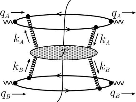
FIG. 5.: Factorized structure of the virtual photon cross section in the high energy limit.

Consider Eq. (69) specialized to the case of two gluon exchange. The approximate gluon four-point function ${\cal G}$ is trivial in this case:

$${\cal G}_{0}(k_{A}^{+},k_{B}^{-},{\bf k}_{A},{\bf k}_{B})={1\over 2}\ \delta({\bf k}_{A}-{\bf k}_{B})\ \delta(k_{A}^{+})\ \delta(k_{B}^{-})\hskip 22.76228pt.$$ (70)

We identify

$$J(0,-{\bf k}_{A};Q_{A}^{2})=G_{1}({\bf k}_{A}^{2}/Q_{A}^{2})\hskip 14.22636pt,\hskip 22.76228ptJ(0,{\bf k}_{B};Q_{B}^{2})=G_{1}({\bf k}_{B}^{2}/Q_{B}^{2})\hskip 14.22636pt.$$ (71)

Then we recover the earlier result (22).

For a generic term in $\cal G$, the transverse momenta ${\bf k}_{A}$ and ${\bf k}_{B}$ are independent variables, while the factor $\delta(k_{A}^{+})\,\delta(k_{B}^{-})$ turns into $1/(k_{A}^{+}k_{B}^{-})$. Taking moments with respect to $s$ and changing integration variables to $\xi_{A}=-k_{A}^{+}/q_{A}^{+}$, $\xi_{B}=k_{B}^{-}/q_{B}^{-}$ and $\lambda=\xi_{A}\xi_{B}s/Q^{2}$ gives the structure

$$\sigma_{N}(Q_{A}^{2},Q_{B}^{2}) = \int{d^{2}{\bf k}_{A}\over\pi{\bf k}_{A}^{2}}\int_{0}^{1}{d\xi_{A}\over\xi_{A}}\ \xi_{A}^{N}\ J(\xi_{A},-{\bf k}_{A};Q_{A}^{2})$$ (73)

$$\times\int{d^{2}{\bf k}_{B}\over\pi{\bf k}_{B}^{2}}\int_{0}^{1}{d\xi_{B}\over\xi_{B}}\ \xi_{B}^{N}\ J(\xi_{B},{\bf k}_{B};Q_{B}^{2})\int_{0}^{\infty}\ {d\lambda\over\lambda}\ \lambda^{-N}\ {\cal H}(\lambda Q^{2},{\bf k}_{A},{\bf k}_{B})\;\;\;.$$

Having evaluated $\cal H$ at some fixed perturbative order, we are interested in the poles of $\sigma_{N}$ at $N=0$. There are poles from the small $\xi_{A}$ and $\xi_{B}$ ends of the integrations over $\xi_{A}$ and $\xi_{B}$. To evaluate $\sigma_{N}$ without losing any powers of $1/N$, we approximate

$$J(\xi_{A},-{\bf k}_{A};Q_{A}^{2}) \to J(0,-{\bf k}_{A};Q_{A}^{2})=G_{1}({\bf k}_{A}^{2}/Q_{A}^{2})\;\;,$$ (74)

$$J(\xi_{B},{\bf k}_{B};Q_{B}^{2}) \to J(0,{\bf k}_{B};Q_{B}^{2})=G_{1}({\bf k}_{B}^{2}/Q_{B}^{2})\;\;.$$ (75)

The pole associated with the integration over $\xi_{A}$ can be thought of as arising from the integration over the rapidity of the final state gluon with the largest rapidity. Almost all of the momentum fraction $\xi_{A}$ is taken by this gluon. Since, in the leading logarithmic approximation, this gluon has a rapidity that is much less than that of the quarks in photon $A$, the momentum fraction $\xi_{A}$ is negligible compared to 1. Similarly, the pole associated with the integration over $\xi_{B}$ can be thought of as arising from the integration over the rapidity of the final state gluon with the most negative rapidity. The poles from the large $\lambda$ end of the integration over the function $\cal H$ can be thought of as arising from integrations over final state gluons with intermediate rapidities.

The leading logarithmic result can thus be written in the form

$$\sigma_{N}(Q_{A}^{2},Q_{B}^{2})=\int{d^{2}{\bf k}_{A}\over\pi{\bf k}_{A}^{2}}\int{d^{2}{\bf k}_{B}\over\pi{\bf k}_{B}^{2}}\ G_{1}({\bf k}_{A}^{2}/Q_{A}^{2})\ {\cal F}_{N}({\bf k}_{A}^{2},{\bf k}_{B}^{2})\ G_{1}({\bf k}_{A}^{2}/Q_{A}^{2})\;\;\;\;,$$ (76)

where ${\cal F}_{N}({\bf k}_{A}^{2},{\bf k}_{B}^{2})$ is the BFKL function that describes the interaction of gluons with fast moving colored systems moving in opposite directions and obeys the BFKL equation [1]. It is normalized so that at order $\alpha_{s}^{0}$ we have

$${\cal F}_{N}^{(0)}({\bf k}_{A}^{2},{\bf k}_{B}^{2})={1\over{2\,N}}\ {1\over\pi}\,\delta({\bf k}_{A}^{2}-{\bf k}_{B}^{2})\;\;\;.$$ (77)

The solution to the BFKL equation can be written to all orders in $\alpha_{s}$ in the form

$${\cal F}_{N}({{\bf k}}_{A}^{2},{{\bf k}}_{B}^{2})={1\over{2\,\,\pi\,\sqrt{{{\bf k}}^{2}_{A}\,{{\bf k}}^{2}_{B}}}}\,\int_{1/2-i\infty}^{1/2+i\infty}\,{{d\,\gamma}\over{2\pi i}}\,\left({{{{\bf k}}^{2}_{A}}\over{{{\bf k}}^{2}_{B}}}\right)^{\gamma-1/2}\,{1\over{N-{\bar{\alpha}_{s}}\,\chi(\gamma)}}\hskip 22.76228pt,$$ (78)

where

$${\bar{\alpha}_{s}}=\alpha_{s}\,C_{A}/\pi\hskip 14.22636pt,\hskip 22.76228ptC_{A}=3\hskip 22.76228pt.$$ (79)

The function $\chi(\gamma)$ is determined by solving the eigenvalue problem for the BFKL kernel and is given by

$$\chi(\gamma)=2\,\psi(1)-\psi(\gamma)-\psi(1-\gamma)\hskip 28.45274pt,$$ (80)

with $\psi$ being the Euler $\psi$-function.

The BFKL function (78) has poles at $N=0$ order by order in perturbation theory. Eq. (76) shows that the poles in the $\gamma^{*}\,\gamma^{*}$ cross section are generated from the ones in ${\cal F}_{N}$ by integrating the color functions over $k_{\perp}$. While these functions are specific to the off-shell photon probe, the function ${\cal F}$ is universal. The same function contributes to the small $x$ behavior of the cross sections in hadron-initiated processes [16] via the high energy factorization formulas.

By inserting the representation (78) in Eq. (76), and scaling out the dependence on the photon virtualities, we get

$${\sigma}_{N}({Q}_{A}^{2},{Q}_{B}^{2})={1\over{2\,\pi\,Q_{A}\,Q_{B}}}\,\int_{1/2-i\infty}^{1/2+i\infty}\,{{d\,\gamma}\over{2\pi i}}\,\left({{{Q}^{2}_{A}}\over{{Q}^{2}_{B}}}\right)^{\gamma-1/2}\,{1\over{N-{\bar{\alpha}_{s}}\,\chi(\gamma)}}\,V_{1}(\gamma)\,V_{1}(1-\gamma)\hskip 22.76228pt,$$ (81)

where $V_{1}(\gamma)$ is defined as the following $k_{\perp}$-transform of the photon color function $G_{1}$

$$V_{1}(\gamma)=\int_{0}^{\infty}\,{{d\,{{\bf k}}^{2}}\over{{{\bf k}}^{2}}}\,\left({{{{\bf k}}^{2}}\over{{Q}^{2}}}\right)^{\gamma-1}\,G_{1}({{{{\bf k}}^{2}}\over{{Q}^{2}}})\hskip 22.76228pt.$$ (82)

The explicit expression of the function $V_{1}(\gamma)$ can be determined by using the representation (31) and performing the integral transform. The result reads

$$V_{1}(\gamma)=\pi\alpha\,\alpha_{s}\,\left(\sum_{q}e^{2}_{q}\right)\,{{(1+\gamma)\,(2-\gamma)\,\Gamma^{2}(\gamma)\,\Gamma^{2}(1-\gamma)}\over{(3-2\,\gamma)\,\Gamma(3/2+\gamma)\,\Gamma(3/2-\gamma)}}\hskip 22.76228pt.$$ (83)

Eq. (81), together with the explicit formulas (80), (83), gives the leading logarithmic result for the moments of the $\gamma^{*}\gamma^{*}$ total cross section. It sums the $1/N$ poles to the accuracy $(\alpha^{2}/N)\times\left(\alpha_{s}/N\right)^{k}$, for any $k$.

The lowest order perturbative contribution, $k=0$, can be recovered from the summed formula (81) by expanding the denominator $\left(N-{\bar{\alpha}_{s}}\,\chi(\gamma)\right)^{-1}$ to the zeroth order in $\alpha_{s}$. The simple pole $N^{-1}$ is the Mellin transform of unity, and one can check numerically that the $\gamma$-integral

$$2\,\pi\,{Q}_{A}\,{Q}_{B}\,{\sigma}^{(0)}({Q}_{A}^{2},{Q}_{B}^{2})=\int_{1/2-i\infty}^{1/2+i\infty}\,{{d\,\gamma}\over{2\pi i}}\,\left({{{Q}^{2}_{A}}\over{{Q}^{2}_{B}}}\right)^{\gamma-1/2}\,V_{1}(\gamma)\,V_{1}(1-\gamma)\hskip 22.76228pt$$ (84)

agrees with Eq. (37) and Fig. 4.

In general, multiple pole contributions $1/N^{k+1}$ to the cross section are obtained by retaining higher orders in the $\alpha_{s}$-expansion of Eq. (81). We see that the general structure of the coefficients of the leading logarithmic series comes from both $\chi(\gamma)$ and $V_{1}(\gamma)$: the former is a universal function associated with the BFKL pomeron, while the latter describes the coupling of the pomeron to a specific physical source.

A Energy dependence

The total cross section is obtained from Eq. (81) by taking the inverse Mellin-Fourier transform (66). By evaluating the $N$-integral from the residue at the pole $N={\bar{\alpha}_{s}}\,\chi(\gamma)$, one gets

$${\sigma}(s,{Q}_{A}^{2},{Q}_{B}^{2})={1\over{2\,\pi\,Q_{A}\,Q_{B}}}\,\int_{1/2-i\infty}^{1/2+i\infty}\,{{d\,\gamma}\over{2\pi i}}\,\left({{{Q}^{2}_{A}}\over{{Q}^{2}_{B}}}\right)^{\gamma-1/2}\left({s\over{Q^{2}}}\right)^{{\bar{\alpha}_{s}}\,\chi(\gamma)}\,V_{1}(\gamma)\,V_{1}(1-\gamma)\hskip 11.38092pt.$$ (85)

Note that this result depends on two mass scales, the scale $\mu^{2}$ in $\alpha_{s}$ and the scale $Q^{2}$ in the high energy corrections, whose reliable determination would require a next-to-leading analysis. We discuss the uncertainties in the leading log result associated with these scales in Secs. V and X.

In the limit $s\to\infty$ the integral (85) is dominated by the region near $\gamma=1/2$, where the function $\chi$ has a saddle point. In the saddle point approximation one obtains

$${\sigma}(s,{Q}_{A}^{2},{Q}_{B}^{2})\simeq{1\over{2\,\pi\,Q_{A}\,Q_{B}}}\,\,{{{|V_{1}(1/2)|}^{2}}\over{\sqrt{2\,\pi\,\chi^{\prime\prime}(1/2)\,{\bar{\alpha}_{s}}\,\ln\left(s/Q^{2}\right)}}}\,\left({s\over{Q^{2}}}\right)^{{\bar{\alpha}_{s}}\,\chi(1/2)}\hskip 22.76228pt,$$ (86)

with

$$\chi(1/2)=4\,\ln 2\simeq 2.77\hskip 5.69046pt,\hskip 11.38092ptV_{1}(1/2)=9\,\pi^{3}\alpha\,\alpha_{s}\,\left(\sum_{q}e^{2}_{q}\right)/8\hskip 5.69046pt,\hskip 11.38092pt\chi^{\prime\prime}(1/2)=28\,\zeta(3)\simeq 33.66\hskip 5.69046pt.$$ (87)

Eq. (86) shows the asymptotic power behavior characteristic of the QCD pomeron, $s^{\lambda}$ with $\lambda={\bar{\alpha}_{s}}\,\chi(1/2)\simeq 2.65\ \alpha_{s}$. The pre-factor that determines the normalization of the asymptotic cross section, on the other hand, depends on the off-shell photon probe, and is controlled by the value of the function $V_{1}(\gamma)$ at $\gamma=1/2$.

If the two photon virtualities are significantly far apart, corrections of order $\ln(Q^{2}_{A}/Q^{2}_{B})/(\alpha_{s}\,\ln(s/Q^{2}))$ need to be taken into account when one calculates the large $s$ limit. In this case, one finds that the position of the saddle point is shifted to $\gamma\simeq 1/2-\ln(Q^{2}_{A}/Q^{2}_{B})/\left({\bar{\alpha}}_{s}\,\chi^{\prime\prime}(1/2)\,\ln(s/Q^{2})\right)$. Apart from corrections in the pre-factor, the net effect of evaluating the integral (85) around the shifted saddle point is to multiply the expression in the right hand side of Eq. (86) by the factor

$$\exp\left[-{{\ln^{2}\left({Q}^{2}_{A}/{Q}^{2}_{B}\right)}\over{2\,\chi^{\prime\prime}(1/2)\,{\bar{\alpha}_{s}}\,\ln\left(s/Q^{2}\right)}}\right]\;\;\;.$$ (88)

The cross section acquires a gaussian modulation in $\ln(Q^{2}_{A}/Q^{2}_{B})$ with a width that grows like $\ln s$.

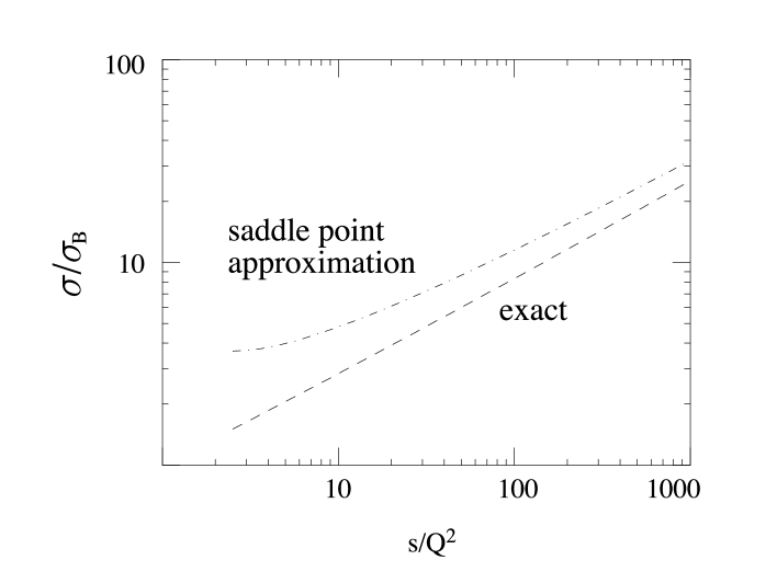
FIG. 6.: The $s/Q^{2}$ dependence of the $\gamma^{*}\,\gamma^{*}$ cross section, Eq. (85). We take $Q_{A}^{2}=Q_{B}^{2}$, $\alpha_{s}=0.2$, and divide $\sigma$ by the Born cross section, which eliminates the factor $1/(Q_{A}Q_{B})$.

In the general case, the integral (85) can be performed numerically. In Fig. 6 we show the result as a function of $s/Q^{2}$ for a given choice of the values of the photon virtualities and the strong coupling. For comparison we also plot the saddle point formula. As the energy increases the two curves get closer. However, in the range considered, the sub-asymptotic contributions are still significant (about $50\%$ at $Q^{2}/s\sim 10^{-1}$, $25\%$ at $Q^{2}/s\sim 10^{-3}$). The large size of the corrections to the saddle point approximation can be mainly traced back to the fact that the function $V_{1}(\gamma)$ itself is rather sharply peaked around $\gamma=1/2$. This is illustrated in Fig. 7, where we see that, for instance, for $\alpha_{s}=0.2$ and $s/Q^{2}=10^{2}$, the width of the pomeron factor is still not small compared to the width of the factor associated with the off-shell photon color function. This effect accounts for most of the shift in the normalization of the cross section between the asymptotic and exact evaluation of the leading logarithmic sum.

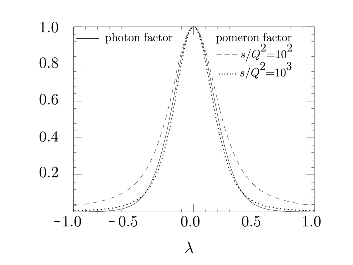
FIG. 7.: The BFKL pomeron factor $\exp\left[{\bar{\alpha}_{s}}\,\,\left(\chi(\gamma)-\chi(1/2)\right)\ln(s/Q^{2})\right]$ and the photon factor $V_{1}(\gamma)\,V_{1}(1-\gamma)/V_{1}^{2}(1/2)$ (normalized to the saddle point) along the contour of integration in Eq. (85). We parametrize this contour as $\gamma=1/2+i\,\lambda$. We take $\alpha_{s}=0.2$, and show the BFKL pomeron factor for two different values $s/Q^{2}=10^{2}$, $s/Q^{2}=10^{3}$.

B Summed results for the asymmetry and the longitudinal cross section

Using the same method described above for the cross section averaged over the two transverse photon polarizations, one can derive summed results for each photon polarization $(1,2,L)$ and for the polarization asymmetry ${\cal A}$. Denoting by $a$, $a^{\prime}$ and $b$, $b^{\prime}$ the polarization indices for photons $q_{A}$ and $q_{B}$, we write the factorization formula for the moments of the polarized cross section $\sigma_{N}^{aa^{\prime},bb^{\prime}}$ as

$$\sigma_{N}^{aa^{\prime},bb^{\prime}}(Q_{A}^{2},Q_{B}^{2})=\int\,{{d^{2}\,{{\bf k}}_{A}}\over{\pi\,{{\bf k}}^{2}_{A}}}\,\int\,{{d^{2}\,{{\bf k}}_{B}}\over{\pi\,{{\bf k}}^{2}_{B}}}\,G^{aa^{\prime}}({{\bf k}}_{A},Q_{A})\,{\widetilde{\cal F}}_{N}({{\bf k}}_{A},{{\bf k}}_{B})\,G^{bb^{\prime}}({{\bf k}}_{B},Q_{B})\,\;\;\;\;.$$ (89)

The color functions $G$ have been discussed in Sec. III. The full solution for the Green’s function ${\widetilde{\cal F}}$ of the BFKL pomeron reads [1]

$${\widetilde{\cal F}}_{N}({{\bf k}}_{A},{{\bf k}}_{B})={1\over{2\,\,\pi\,\sqrt{{{\bf k}}^{2}_{A}\,{{\bf k}}^{2}_{B}}}}\,\sum_{m=-\infty}^{+\infty}\int_{1/2-i\infty}^{1/2+i\infty}\,{{d\,\gamma}\over{2\pi i}}\,{1\over{N-{\bar{\alpha}_{s}}\,\chi_{m}(\gamma)}}\,\left({{{{\bf k}}^{2}_{A}}\over{{{\bf k}}^{2}_{B}}}\right)^{\gamma-1/2}\,e^{i\,m\,(\phi_{A}-\phi_{B})}\hskip 2.84544pt$$ (90)

with

$$\chi_{m}(\gamma)=2\,\psi(1)-\psi(\gamma+|m|/2)-\psi(1-\gamma+|m|/2)\hskip 28.45274pt.$$ (91)

The function ${\cal F}$ in Eq. (78), relevant to the case of the unpolarized cross section, is given by the term $m=0$ in Eq. (90).

Consider the product $\Sigma={\overline{\sigma}}\,{\cal A}$ of the asymmetry times the averaged cross section, with the asymmetry ${\cal A}$ defined in Eq. (56). Due to the azimuthal integration only the terms with $m=+2,-2$ in Eq. (90) contribute. Substituting the color function $G_{2}$ (see Eq. (51)) in Eq. (89), one finds for the $N$ moments

$$\Sigma_{N}({Q}_{A}^{2},{Q}_{B}^{2})={1\over{16\,\pi\,Q_{A}\,Q_{B}}}\,\int_{1/2-i\infty}^{1/2+i\infty}\,{{d\,\gamma}\over{2\pi i}}\,\left({{{Q}^{2}_{A}}\over{{Q}^{2}_{B}}}\right)^{\gamma-1/2}\,{1\over{N-{\bar{\alpha}_{s}}\,\chi_{2}(\gamma)}}\,V_{2}(\gamma)\,V_{2}(1-\gamma)\hskip 22.76228pt,$$ (92)

where $V_{2}(\gamma)$ is defined from the $k_{\perp}$-transform of the function $G_{2}$ analogous to (82), and has the expression

$$V_{2}(\gamma)=2\,\pi\alpha\,\alpha_{s}\,\left(\sum_{q}e^{2}_{q}\right)\,{{\Gamma(1+\gamma)\,\Gamma(2-\gamma)\,\Gamma(\gamma)\,\Gamma(1-\gamma)}\over{(3-2\,\gamma)\,\Gamma(3/2+\gamma)\,\Gamma(3/2-\gamma)}}\hskip 22.76228pt.$$ (93)

By inverse Mellin-Fourier transformation, one obtains the summed formula for the asymmetry in the energy space:

$${\cal A}(s,{Q}_{A}^{2},{Q}_{B}^{2}) = {1\over{{\overline{\sigma}}(s,Q_{A}^{2},Q_{B}^{2})}}\,{1\over{16\,\pi\,Q_{A}\,Q_{B}}}$$ (95)

$$\times\,\int_{1/2-i\infty}^{1/2+i\infty}\,{{d\,\gamma}\over{2\pi i}}\,\left({{{Q}^{2}_{A}}\over{{Q}^{2}_{B}}}\right)^{\gamma-1/2}\left({s\over{Q^{2}}}\right)^{{\bar{\alpha}_{s}}\,\chi_{2}(\gamma)}\,V_{2}(\gamma)\,V_{2}(1-\gamma)\hskip 11.38092pt,$$

where ${\overline{\sigma}}$ is given by Eq. (85).

As in the case of the unpolarized cross section, the asymptotic behavior in the limit $s\to\infty$ is determined by the saddle point approximation to the integral in Eq. (95). In this case we observe a negative power law with the energy $s$, controlled by the value of $\chi_{2}$ at the saddle point, $\chi_{2}(1/2)=-4\,(1-\ln 2)\simeq-1.23$, indicating that the angular correlations between the two photons tend to be washed out when BFKL pomeron exchange dominates.

The contributions to the photon-photon cross section from longitudinally polarized photons are given by formulas analogous to Eq. (85) in terms of different combinations of the functions $V_{1}$ and $V_{2}$, and the same function $\chi$:

$${\sigma}^{(LL)}(s,{Q}_{A}^{2},{Q}_{B}^{2})={1\over{2\,\pi\,Q_{A}\,Q_{B}}}\,\int_{1/2-i\infty}^{1/2+i\infty}\,{{d\,\gamma}\over{2\pi i}}\,\left({{{Q}^{2}_{A}}\over{{Q}^{2}_{B}}}\right)^{\gamma-1/2}\left({s\over{Q^{2}}}\right)^{{\bar{\alpha}_{s}}\,\chi(\gamma)}\,V_{2}(\gamma)\,V_{2}(1-\gamma)\hskip 5.69046pt,$$ (96)

$${\sigma}^{(TL)}(s,{Q}_{A}^{2},{Q}_{B}^{2})={\sigma}^{(LT)}(s,{Q}_{A}^{2},{Q}_{B}^{2})$$ (97)

$$={1\over{2\,\pi\,Q_{A}\,Q_{B}}}\,\int_{1/2-i\infty}^{1/2+i\infty}\,{{d\,\gamma}\over{2\pi i}}\,\left({{{Q}^{2}_{A}}\over{{Q}^{2}_{B}}}\right)^{\gamma-1/2}\left({s\over{Q^{2}}}\right)^{{\bar{\alpha}_{s}}\,\chi(\gamma)}\,V_{1}(\gamma)\,V_{2}(1-\gamma)\hskip 5.69046pt.$$ (98)

Unlike $V_{1}(\gamma)$ in Eq. (83), $V_{2}$ has simple poles at $\gamma=0,1$ (instead of double poles), corresponding to the non-logarithmic behavior of the color function $G_{2}$ at ${{\bf k}}^{2}\ll Q^{2}$, ${{\bf k}}^{2}\gg Q^{2}$ noted in Sec. III. Replacing functions $V_{1}$ by functions $V_{2}$ accounts for the different size of the longitudinal cross sections with respect to the purely transverse one. Roughly, one finds

$${\sigma}^{(LL)}\approx 0.05\;{\sigma}^{(TT)}\hskip 5.69046pt,\hskip 11.38092pt{\sigma}^{(TL)}\approx 0.2\;{\sigma}^{(TT)}\hskip 5.69046pt.$$ (99)

V Scale dependence and uncertainties of the leading logarithmic approximation

The result (85) for the $\gamma^{*}\,\gamma^{*}$ cross section depends on two mass scales which cannot be determined in a leading logarithmic analysis: the mass $\mu^{2}$ at which the running coupling $\alpha_{s}$ is evaluated, and the mass $Q^{2}$ that provides the scale for the high energy logarithms. The former can be thought of as being associated with the integrations over the transverse momenta in the loops contributing to higher order diagrams, while the latter stems from the longitudinal integrations. A reliable determination of these scales would require a next-to-leading order calculation. Lacking this, we provide here qualitative arguments to relate these scales with the physical hard scales of the problem. In Sec. X we will use these relations to examine numerically the dependence of the cross section on the scale choices.

A possible choice of the scale $\mu^{2}$ in the strong coupling is based on the prescription of Ref. [17]. To apply this prescription, we consider the lowest order gluon exchange contribution, which we have discussed in Sec. II. This is given (see Eq. (22)) by the integral in $d{{\bf k}}^{2}$ of two $G$ factors, each of which is proportional to $\alpha_{s}$, $G=\alpha_{s}(\mu^{2})\,{\cal G}$. We first compute the quark loop contribution to the gluon propagator, renormalized in the ${\overline{\mbox{MS}}}$ scheme:

$$\Pi({\bf k}^{2})={\tilde{\beta}}_{0}\,\left[\ln({{\bf k}}^{2}/\mu^{2})+C\right]\;\;\;\;,$$ (100)

where ${\tilde{\beta}}_{0}=-1/(6\,\pi)$ is the contribution to $\beta_{0}=(33-2\,N_{f})/(12\,\pi)$ from one quark loop, and $C=-5/3$. Inserting a quark loop into the gluon propagator in the lowest order diagram amounts to replacing $\alpha_{s}(\mu^{2})$ by

$$\alpha_{s}(\mu^{2})\left[1-{\tilde{\beta}}_{0}\,\alpha_{s}(\mu^{2})\,\ln({{\bf k}}^{2}\,e^{C}/\mu^{2})\right]$$ (101)

(as in [17] this can be regarded as a contribution to an effective coupling $\alpha_{eff}({{\bf k}}^{2})$). Now, following [17] we choose the scale $\mu^{2}$ so that the quark loop contribution vanishes after integrating over ${{\bf k}}^{2}$:

$$\int_{0}^{\infty}{{d{{\bf k}}^{2}}\over{({{\bf k}}^{2})^{2}}}\,{\cal G}({{\bf k}}^{2}/Q^{2}_{A})\,{\cal G}({{\bf k}}^{2}/Q^{2}_{B})\,\ln({{\bf k}}^{2}\,e^{C}/\mu^{2})=0\;\;\;\;.$$ (102)

This is the same procedure that applies in the case of the abelian theory. Using the representation (31) for $G$, we are led to calculate an integral of the form

$$\int_{0}^{\infty}{d{{\bf k}}^{2}}{1\over{\lambda_{A}\,(1-\lambda_{A})\,{{\bf k}}^{2}+z_{A}\,(1-z_{A})\,Q^{2}_{A}}}\,{1\over{\lambda_{B}\,(1-\lambda_{B})\,{{\bf k}}^{2}+z_{B}\,(1-z_{B})\,Q^{2}_{B}}}\,\ln\left({{{{\bf k}}^{2}\,e^{C}}\over{\mu^{2}}}\right)\;\;\;\;.$$ (103)

Exploiting the symmetry of the integrand under the transformation ${{\bf k}}^{2}/Q_{A}\,Q_{B}\to Q_{A}\,Q_{B}/{{\bf k}}^{2}$ and interchange of the variables $z_{A}\leftrightarrow\lambda_{B}$, $z_{B}\leftrightarrow\lambda_{A}$, one can show that the condition (102) is satisfied by

$$\mu^{2}=c_{\mu}\,Q_{A}\,Q_{B}\hskip 14.22636pt,\hskip 17.07182ptc_{\mu}=e^{-5/3}\hskip 14.22636pt.$$ (104)

Note that, when the two photon virtualities $Q_{A}^{2}$ and $Q_{B}^{2}$ are far apart from each other, the prescription [17] picks out a scale for $\alpha_{s}$ which is neither of the order of the big virtuality nor of the order of the small one, but rather is proportional to the geometric mean $\sqrt{Q_{A}^{2}\,Q_{B}^{2}}$. The value of the proportionality coefficient $c_{\mu}$ in Eq. (104) is specific to the subtraction scheme (${\overline{\mbox{MS}}}$) chosen to define the quark loop insertion.

The argument given above applies to the factors of $\alpha_{s}$ that appear in the Born approximation to the high energy cross section. The result (85), however, also contains a dependence on the running coupling through the higher order factor $s^{\alpha_{s}\,\chi}$ associated with the solution of the BFKL equation. For the scale in $\alpha_{s}$ in this case one does not have such a simple argument as the one described above. For the numerical estimates in Sec. X we will make the assumption that the same value of $\mu^{2}$ also controls the running coupling in the BFKL factor. In Sec. X we will check the numerical effect of varying this scale.

We now consider the mass $Q^{2}$ that provides the scale for the large energy logarithms $\left(\alpha_{s}\ln(s/Q^{2})\right)^{k}$ (see Eq. (65)). To estimate this scale, we observe that the rapidity of gluons exchanged in the rungs of the BFKL ladders should lie between the rapidity $y_{A}$ of the quark $p_{A}$ (produced by the photon $q_{A}$) and the rapidity $y_{B}$ of the quark $p_{B}$ (produced by the photon $q_{B}$). This gives rise to integrations over the rapidity intervals

$$\int_{y_{B}}^{y_{A}}dy=y_{A}-y_{B}\hskip 8.5359pt.$$ (105)

The logarithms of the energy $s$ are generated precisely by these integrals. Estimating the size of the rapidity intervals thus allows us to estimate the scale $Q^{2}$.

Expressing the “$+$” and “$-$” momentum components of the quark $p_{A}$ as

$$p_{A}^{+}=z_{A}\,q^{+}_{A}\hskip 8.5359pt,\hskip 14.22636ptp_{A}^{-}={{{\bf p}}_{\perp\,A}^{2}\over{2\;p^{+}_{A}}}\hskip 14.22636pt,$$ (106)

we write its rapidity as

$$y_{A}={1\over 2}\ln\left({{p_{A}^{+}}\over{p_{A}^{-}}}\right)={1\over 2}\ln\left({{2\,z_{A}^{2}\,(q^{+}_{A})^{2}}\over{{{\bf p}}_{\perp\,A}^{2}}}\right)\hskip 14.22636pt.$$ (107)

Similarly, for the quark $p_{B}$ we have

$$y_{B}={1\over 2}\ln\left({{p_{B}^{+}}\over{p_{B}^{-}}}\right)=-{1\over 2}\ln\left({{2\,z_{B}^{2}\,(q^{-}_{B})^{2}}\over{{{\bf p}}_{\perp\,B}^{2}}}\right)\hskip 14.22636pt.$$ (108)

Taking the difference between these rapidities gives

$$y_{A}-y_{B}=\ln\left({{z_{A}\,z_{B}\,s}\over{|{{\bf p}}_{\perp\,A}|\,|{{\bf p}}_{\perp\,B}|}}\right)\;\;\;\;\;.$$ (109)

The average transverse momenta ${{\bf p}}_{\perp\,A}$, ${{\bf p}}_{\perp\,B}$ carried by the quarks are of the order of the photon virtualities $Q_{A}$, $Q_{B}$. For the longitudinal momentum fractions $z_{A}$, $z_{B}$, we assume a typical maximum value of the order $z_{\rm max}\sim 0.1$ in the high energy region. Using these estimates, we obtain

$$y_{A}-y_{B}=\ln\left({{s\,z_{\rm max}^{2}}\over{Q_{A}\,Q_{B}}}\right)\;\;\;\;\;.$$ (110)

We thus identify the scale

$$Q^{2}=c_{Q}\,Q_{A}\,Q_{B}\hskip 14.22636pt,\hskip 17.07182ptc_{Q}=1/z_{\rm max}^{2}=10^{2}\hskip 14.22636pt.$$ (111)

VI Limitations on the BFKL pomeron approach at very large energy

The transverse-momentum integrations in the factorization formula (76) are dominated by values of ${{\bf k}}^{2}_{A},{{\bf k}}^{2}_{B}$ of the order of the photon virtualities. (For the purpose of this section we will take the photon virtualities to be equal, ${Q}^{2}_{A}={Q}^{2}_{B}$.) As a result, for sufficiently off shell photons the dominant contribution to the cross section comes from short distances, and the evaluation of Eq. (76) gives rise to a finite result in perturbation theory. However, there are limitations on the perturbative treatment that are intrinsic to the BFKL equation. These limitations come from the region of very high $s$. Although an accurate understanding of these effects is an open problem [18] that goes beyond the scope of this work, one can nevertheless make some rough estimates. We discuss them in this section. In order to keep the notation simple, we do not distinguish here between the scales $Q_{A}Q_{B}$, $Q^{2}=c_{Q}Q_{A}Q_{B}$, and $\mu^{2}=c_{\mu}Q_{A}Q_{B}$, calling all of these simply $Q^{2}$.

It is known from the structure of the BFKL equation that, even if the incoming ${{\bf k}}^{2}_{A}$, ${{\bf k}}^{2}_{B}$ are large, say, ${{\bf k}}^{2}_{A},{{\bf k}}^{2}_{B}\sim Q^{2}$, the typical transverse momenta in the gluon ladders contributing to the function ${\cal F}_{N}({{\bf k}}_{A},{{\bf k}}_{B})$ (see Eq. (78)) may diffuse away from $Q^{2}$ as the energy becomes very large. The diffusion coefficient in $\ln{{\bf k}}^{2}$ can be read directly from the asymptotic solution to the BFKL equation (or, equivalently, from the exponential term (88) in the $\gamma^{*}\,\gamma^{*}$ cross section) and is given by

$$\rho_{\rm diff}=2\,\chi^{\prime\prime}(1/2)\,{\bar{\alpha}_{s}}\,\ln\left(s/Q^{2}\right)\,\;\;.$$ (112)

As a result, the distribution of the transverse momenta in the BFKL ladders is a gaussian in $\ln{{\bf k}}^{2}$ centered around $Q^{2}$ with a width proportional to $\rho_{\rm diff}$ [19]. With increasing $s$ the distribution broadens, and one becomes sensitive to the region of small transverse momenta.

A self-consistency check of the perturbative treatment requires that the contribution from transverse momenta of the order of $\Lambda_{QCD}$ be suppressed. In order to keep away from momenta of this order one has to have

$$\ln^{2}(Q^{2}/\Lambda^{2})/\left(2\,\chi^{\prime\prime}(1/2)\,{\bar{\alpha}_{s}}\,\ln(s/Q^{2})\right)\gtrsim 1\;\;\;\;.$$ (113)

Identifying $\alpha_{s}$ with the strong coupling evaluated at the scale $Q^{2}$, $\alpha_{s}\simeq\left(\beta_{0}\,\ln(Q^{2}/\Lambda^{2})\right)^{-1}$, one gets

$$\alpha_{s}(Q^{2})\,\ln(s/Q^{2})\lesssim c_{1}/\alpha_{s}^{2}(Q^{2})\;\;,\hskip 34.14322ptc_{1}=\pi/\left(2\,\chi^{\prime\prime}(1/2)\,\beta_{0}^{2}\,C_{A}\right)\approx 1/30\;\,.$$ (114)

For any given $Q^{2}$, this can be read as an upper bound on the domain of energies $s$ in which we expect the perturbative approach based on the BFKL pomeron to be reliable. Observe that, for small values of $\alpha_{s}$, this is not so stringent a constraint. However, because the BFKL function $\chi$ has a large second derivative at the saddle point, the numerical value of the coefficient $c_{1}$ is small. Therefore, the limit (114) may become relevant unless $Q^{2}$ is very large.

The BFKL equation is also known to give rise to violation of the unitarity bound at asymptotically large energies. The growth of the cross section predicted by the BFKL equation cannot continue indefinitely, and unitarity corrections must arise to slow it down. Roughly, these effects are expected to become important when the calculated cross section is bigger than the naive geometrical cross section $1/Q^{2}$. A careful discussion may be found in Ref. [20]. The simplest estimate, $\sigma\lesssim 1/Q^{2}$, yields, using Eq. (86),

$${{\alpha_{s}^{2}}\over{\sqrt{2\,\pi\,\chi^{\prime\prime}(1/2)\,{\bar{\alpha}_{s}}\,\ln\left(s/(Q^{2})\right)}}}\,\left({s\over{Q^{2}}}\right)^{{\bar{\alpha}_{s}}\,\chi(1/2)}\lesssim 1\;\;\;\;,$$ (115)

where we have neglected factors from the term in $V_{1}(1/2)$ in Eq. (86). Assuming, as we did before, $\alpha_{s}$ to be evaluated at the scale $Q^{2}$, we can write

$$\alpha_{s}(Q^{2})\,\ln(s/Q^{2})\lesssim c_{2}\,\ln(1/\alpha_{s}^{2}(Q^{2}))+A\;\;,\hskip 34.14322ptc_{2}=\pi/\left(C_{A}\,\chi(1/2)\right)\approx 1/3\;\,.$$ (116)

In the term $A$ we collect contributions arising from the factor in the square root in Eq. (115) as well as from the factor $V_{1}$ in Eq. (86).

The different functional dependence on $\alpha_{s}$ in the right hand sides of the inequalities (114) and (116) implies that, for small enough values of $\alpha_{s}$, the unitarity limit (116) is more stringent than the diffusion limit (114). This suggests that for sufficiently high $Q^{2}$ it should be possible to study unitarization in a purely perturbative context [20].

On the other hand, the coefficients $c_{1}$ and $c_{2}$ are significantly different in size. This may make the two bounds (114) and (116) rather comparable for moderate values of $Q^{2}$. In addition, inspection of Eqs. (86), (115) suggests that the term $A$ in Eq. (116) is not necessarily negligible, and may contribute to push the onset of unitarity corrections further away.

As to the impact on experimental studies at future $e^{+}e^{-}$ colliders, we observe that unitarity corrections should set in when the cross section has grown to be much larger than the Born value $\sim\alpha_{s}^{2}/Q^{2}$. At a future $e^{+}e^{-}$ collider one may thus expect to see the rise of the cross section with $s/Q^{2}$. Possibly, one may see this rise slow as unitarity corrections become important [10].

VII Virtuality dependence and relationship with deeply inelastic scattering

If we let $Q_{A}^{2}$ be much larger than $Q_{B}^{2}$ in Eq. (85), we obtain a result that describes small $x$ deeply inelastic scattering from a transversely polarized photon [21] whose virtuality $Q_{B}^{2}$ is sufficiently large to allow the use of perturbation theory to analyze its decomposition into quarks. The structure function $F_{1}(x,Q^{2})$ (which is the same as $F_{T}$) is related to the virtual photon-photon cross section by

$$F_{1}(x,Q_{A}^{2})={1\over(2\pi)^{2}\alpha}\ Q_{A}^{2}\ {\sigma}(s,{Q}_{A}^{2},{Q}_{B}^{2})$$ (117)

with

$$s={Q_{A}^{2}\over x}\;\;\;.$$ (118)

Thus Eq. (85) gives a leading logarithmic summation for $F_{1}$ at small $x$:

$$F_{1}(x,Q_{A}^{2})={1\over(2\pi)^{3}\alpha}\,\int_{1/2-i\infty}^{1/2+i\infty}\,{{d\,\gamma}\over{2\pi i}}\,\left({{{Q}^{2}_{A}}\over{{Q}^{2}_{B}}}\right)^{\gamma}\left(Q_{A}^{2}\over x\,Q^{2}\right)^{{\bar{\alpha}_{s}}\,\chi(\gamma)}\,V_{1}(\gamma)\,V_{1}(1-\gamma)\hskip 11.38092pt.$$ (119)

The scale $Q^{2}$ is not fixed by a leading logarithmic calculation. A sensible choice for $Q^{2}$ based on a qualitative argument has been discussed in Sec. V. For the purpose of the present section we simply leave it undetermined.

Consider the perturbative expansion of Eq. (119),

$$F_{1}(x,Q_{A}^{2})={1\over(2\pi)^{3}\alpha}\,\int_{1/2-i\infty}^{1/2+i\infty}\,{{d\,\gamma}\over{2\pi i}}\,\left({{{Q}^{2}_{A}}\over{{Q}^{2}_{B}}}\right)^{\gamma}\left[1+{\bar{\alpha}_{s}}\,\chi(\gamma)\ln\left(Q_{A}^{2}\over x\,Q^{2}\right)+\cdots\right]\,V_{1}(\gamma)\,V_{1}(1-\gamma)\hskip 2.84544pt.$$ (120)

The functions $V_{1}(\gamma)$, $V_{1}(1-\gamma)$ and $\chi(\gamma)$ have poles at integer values of $\gamma$. Thus this expression contains contributions proportional to $(Q_{A}^{2})^{0}$ times logarithms, $(Q_{A}^{2})^{-1}$ times logarithms, and so forth. We extract the leading twist contribution, the part proportional to $(Q_{A}^{2})^{0}$ times logarithms, by rewriting the integral as an integral over a contour $\cal C$ that encircles the singularity at $\gamma=0$ plus an integral over a contour from $-1/2-i\infty$ to $-1/2+i\infty$. The integral over the contour $\cal C$ is the leading twist contribution. We discard the integration over the contour from $-1/2-i\infty$ to $-1/2+i\infty$, which contains the higher twist contributions. Thus the leading twist contribution to $F_{1}$ is

$$F_{1}^{\rm L.T.}(x,Q_{A}^{2}) = {1\over(2\pi)^{3}\alpha}\,\int_{\cal C}\,{{d\,\gamma}\over{2\pi i}}\,\left({{{Q}^{2}_{A}}\over{{Q}^{2}_{B}}}\right)^{\gamma}\left[1+{\bar{\alpha}_{s}}\,\chi(\gamma)\ln\left(Q_{A}^{2}\over x\,Q^{2}\right)+\cdots\right]\,V_{1}(\gamma)\,V_{1}(1-\gamma)$$ (121)

$$= {1\over(2\pi)^{3}\alpha}\ {\lower 6.0pt\hbox{\vbox{\hbox{$\rm Res$} \kern-6.0pt\hbox{$\scriptstyle\,\gamma=0$}}}}\,\left({{{Q}^{2}_{A}}\over{{Q}^{2}_{B}}}\right)^{\gamma}\left[1+{\bar{\alpha}_{s}}\,\chi(\gamma)\ln\left(Q_{A}^{2}\over x\,Q^{2}\right)+\cdots\right]\,V_{1}(\gamma)\,V_{1}(1-\gamma)\hskip 2.84544pt.$$ (122)

It is straightforward to determine the perturbative coefficients. The function $V_{1}(\gamma)$ has a double pole at $\gamma=0$, as does the function $V_{1}(1-\gamma)$. Thus there are three powers of $\ln(Q_{A}^{2}/Q_{B}^{2})$ at leading order in $\alpha_{s}$, which is $\alpha_{s}^{2}$ since $V_{1}\propto\alpha_{s}$. We find

$$F_{1}^{\rm L.T.}(x,Q_{A}^{2}) = {{4\,\alpha\,\alpha_{s}^{2}}\over{9\,\pi^{3}}}\,\left(\sum_{q}e^{2}_{q}\right)^{2}\,\left[{1\over 3}\,\ln^{3}\!\left({{Q_{A}^{2}}\over{Q_{B}^{2}}}\right)+{7\over 3}\,\ln^{2}\!\left({{Q_{A}^{2}}\over{Q_{B}^{2}}}\right)+\left({119\over 6}-4\,\zeta(2)\right)\,\ln\!\left({{Q_{A}^{2}}\over{Q_{B}^{2}}}\right)\right.$$ (124)

$$\left.+\left({1063\over 27}-{28\over 3}\,\zeta(2)\right)\,+{\cal O}\left(\alpha_{s}\right)\right]\hskip 5.69046pt,\hskip 11.38092pt\zeta(2)\simeq 1.64\hskip 5.69046pt.$$

If we restore the summation of the leading logs of $1/x$, we obtain

$$F_{1}^{\rm L.T.}(x,Q_{A}^{2})={1\over(2\pi)^{3}\alpha}\,\int_{\cal C}\,{{d\,\gamma}\over{2\pi i}}\,\left({{{Q}^{2}_{A}}\over{{Q}^{2}_{B}}}\right)^{\gamma}\left({Q_{A}^{2}\over x{Q^{2}}}\right)^{{\bar{\alpha}_{s}}\,\chi(\gamma)}\,V_{1}(\gamma)\,V_{1}(1-\gamma)\hskip 11.38092pt.$$ (125)

This is not a simple function. However, one can easily perform the integration numerically.

One interesting result is that we observe what used to be called “precocious Bjorken scaling”. That is, the leading twist approximation begins to be accurate at values of $Q_{A}^{2}$ that are not really very large compared to the only other scale in the problem, $Q_{B}^{2}$. We illustrate this in Fig. 8, working at order $\alpha_{s}^{2}$. We compare the leading twist approximation that applies for $Q_{A}^{2}\gg Q_{B}^{2}$, the leading twist approximation that applies for $Q_{B}^{2}\gg Q_{A}^{2}$, and the full result. First we define $x_{A}=Q_{A}^{2}/s$ and plot

$$\sigma_{\rm L.T.-A}(s,Q_{A}^{2},Q_{B}^{2})={{(2\pi)^{2}\alpha}\over Q_{A}^{2}}\ F_{1}^{\rm L.T.}(x_{A},Q_{A}^{2})$$ (126)

versus $Q_{A}/Q_{B}$. Then we define $x_{B}=Q_{B}^{2}/s$ and plot

$$\sigma_{\rm L.T.-B}(s,Q_{A}^{2},Q_{B}^{2})={{(2\pi)^{2}\alpha}\over Q_{B}^{2}}\ F_{1}^{\rm L.T.}(x_{B},Q_{B}^{2})$$ (127)

Finally, we plot $\sigma(s,Q_{A}^{2},Q_{B}^{2})$ at the leading order in $\alpha_{s}$ without approximation. We see that the leading twist approximation for $Q_{A}^{2}\gg Q_{B}^{2}$ is quite good down to $Q_{A}^{2}=Q_{B}^{2}$, while the leading twist approximation that applies for $Q_{B}^{2}\gg Q_{A}^{2}$ is quite good down to $Q_{B}^{2}=Q_{A}^{2}$. In fact, at $Q_{A}^{2}=Q_{B}^{2}$, both approximations are quite good. A similar behavior is observed if we include higher orders in $\alpha_{s}$.

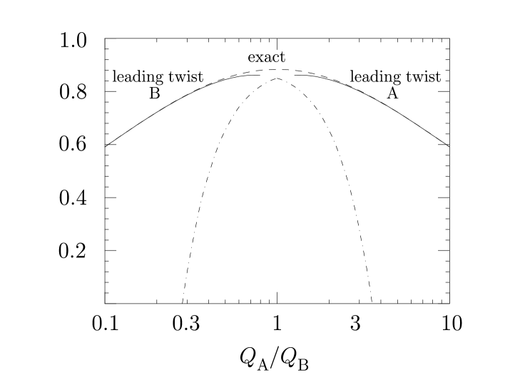
FIG. 8.: The full and the leading-twist approximation to the virtual photon cross section. We plot the cross section divided by $16\alpha^{2}\alpha_{s}^{2}(\sum_{q}e_{q}^{2})^{2}/(Q_{A}Q_{B})$, as in Fig. 4.

VIII Regge factorization

The QCD result for $\gamma^{*}\,\gamma^{*}$ scattering can be compared with expectations for the structure of the high energy cross section based on traditional Regge theory [22]. In Regge theory, to analyze the elastic scattering of particles $A$ and $B$ one considers the singularity structure of the amplitude $A(s,t)$ in the complex angular momentum plane. The simplest case is a pole in the angular momentum $j$ plane located at a position dependent on $t$, $1/\left(j-\alpha(t)\right)$. One then obtains the asymptotic behavior $s^{\alpha(t)}$ for $s\to\infty$ and $t$ fixed, and the amplitude takes the factorized form

$$A(s,t)\sim\beta_{A}(t)\,s^{\alpha(t)}\,\beta_{B}(t)\hskip 11.38092pt.$$ (128)

Here $\beta_{A}$, $\beta_{B}$ are functions of the transferred momentum, associated respectively with the couplings of particles $A$ and $B$ to the reggeon whose trajectory is ${\alpha(t)}$.

For the case of the $\gamma^{*}\,\gamma^{*}$ total cross section, this would correspond to the structure

$$\sigma_{\gamma^{*}\,\gamma^{*}}(s,Q^{2}_{A},Q^{2}_{B})\sim\beta_{A}(t=0;Q^{2}_{A})\,s^{\alpha(0)-1}\,\beta_{B}(t=0;Q^{2}_{B})\hskip 11.38092pt,$$ (129)

where we have used the optical theorem to relate the total cross section to the imaginary part of the forward elastic amplitude, and we have let $\beta_{A}$ and $\beta_{B}$ depend on the photon virtualities in the case of off-shell photons.

However, it has been long known, from various phenomenological and theoretical considerations [22], that this structure cannot be exactly true, and strong-interaction scattering at high energy has to have a more complicated singularity structure than a pole, such as moving or fixed cuts. In this case, one does not expect the factorized form for the cross section to hold.

If we now turn to the QCD result (see Eq. (81)), we may ask what kind of singularities the amplitude has in the angular momentum plane. The BFKL pomeron is known to give rise to a (fixed) branch point singularity [1]. To see this, let us consider the moments of the $\gamma^{*}\,\gamma^{*}$ cross section. At leading level, we are allowed to identify the moment $N$ with the complex angular momentum $j$ [22]. Eq. (81) is written in terms of an integral in the complex $\gamma$-plane. The integrand has the pole $1/\left(N-{\bar{\alpha}}_{s}\,\chi(\gamma)\right)$ and one factor of $V$ for the coupling of the gluon system to the quarks in each photon. Thus the integrand has a factorized structure. To understand the angular-momentum singularity structure, one should see what becomes of the pole $N={\bar{\alpha}}_{s}\,\chi(\gamma)$ after $\gamma$-integration.

For $Q_{A}^{2}>Q_{B}^{2}$, the $\gamma$-integral is well approximated by the residue at the rightmost pole ${\bar{\gamma}}$ to the left of the integration contour. As we have seen in the previous section, numerically this approximation turns out to be fairly good down to values of $Q_{A}^{2}/Q_{B}^{2}$ just above $1$. In this approximation one gets

$${\sigma}_{N}(Q_{A}^{2},Q_{B}^{2})\sim{1\over{2\,\pi\,Q_{A}^{2}}}\,C_{N}\,\exp\left[{\bar{\gamma}}_{N}\,\ln(Q_{A}^{2}/Q_{B}^{2})\right]\;\;,\;\;\;C_{N}=-{{V_{1}({\bar{\gamma}}_{N})\,V_{1}(1-{\bar{\gamma}}_{N})}\over{{\bar{\alpha}}_{s}\,\chi^{\prime}({\bar{\gamma}}_{N})}}\;\;\;.$$ (130)

The leading pole ${\bar{\gamma}}_{N}$ is determined by the equation $N-{\bar{\alpha}}_{s}\,\chi({\bar{\gamma}})=0$. At $N={\bar{\alpha}}_{s}\,\chi(1/2)$ it has a square-root branch point singularity:

$${\bar{\gamma}}_{N}\sim{1\over 2}-\sqrt{{{2\,\left(N-N_{0}\right)}\over{{\bar{\alpha}}_{s}\,\chi^{\prime\prime}(1/2)}}}\;\;,\;\;\;N\to N_{0}\equiv{\bar{\alpha}}_{s}\,\chi(1/2)\;\;\;.$$ (131)

Correspondingly, the residue $C_{N}$ is also singular:

$$C_{N}\sim|V_{1}(1/2)|^{2}/\sqrt{2\,{\bar{\alpha}}_{s}\,\chi^{\prime\prime}(1/2)\,\left(N-N_{0}\right)}\;\;,\;\;\;N\to N_{0}\;\;\;.$$ (132)

Therefore, the QCD result implies a branch point rather than a simple pole in the angular momentum plane. As a consequence, we do not obtain a Regge-factorized form for $\sigma(s,Q_{A}^{2},Q_{B}^{2})$.

It is of interest, however, to see by how much this factorization is violated. We first consider the asymptotic formula (86), obtained by using the saddle point approximation around $\gamma=1/2$. In this case, provided the scale $Q^{2}$ is fixed by $Q^{2}=c_{Q}\,Q_{A}\,Q_{B}$, as discussed in Sec. V, and the QCD coupling $\alpha_{s}$ is fixed, an approximate form of Regge factorization is recovered. The piece which violates this factorization in Eq. (86) is proportional to the square root of a logarithm, and is therefore a slowly varying function. A more substantial source of factorization breaking comes in when one takes into account the correction due to the position of the saddle point drifting away from $1/2$, see Eq.(88).

For the exact leading log result (85), a possible way to quantify the deviation from the Regge-factorized behavior is to look at the ratio

$$R={{\left[\sigma_{\gamma^{*}\,\gamma^{*}}(s,Q^{2}_{A},Q^{2}_{B})\right]^{2}}\over{\sigma_{\gamma^{*}\,\gamma^{*}}(s,Q^{2}_{A},Q^{2}_{A})\,\sigma_{\gamma^{*}\,\gamma^{*}}(s,Q^{2}_{B},Q^{2}_{B})}}\hskip 14.22636pt.$$ (133)

If Regge factorization holds, this quantity should be equal to $1$. On the other hand, from Eq. (85) we see that $R$ goes like $R\sim Q_{B}^{2}/Q_{A}^{2}$ for $Q_{A}^{2}\gg Q_{B}^{2}$, and $R\sim Q_{A}^{2}/Q_{B}^{2}$ for $Q_{B}^{2}\gg Q_{A}^{2}$. That is, for $Q_{A}$ and $Q_{B}$ sufficiently far apart the Regge-factorized form breaks down.

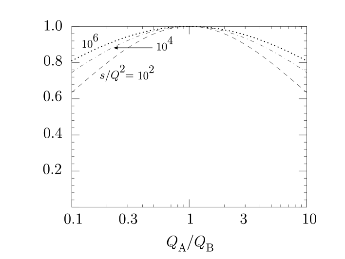
FIG. 9.: The $Q_{A}/Q_{B}$ dependence of the ratio $R$ defined in Eq. (133), at different values of $s/Q^{2}$.

In Fig. 9, we plot $R$ as a function of the ratio of the photon virtualities $Q_{A}/Q_{B}$ for different values of the energy. It is interesting to observe that, for typical parameter values, $R$ varies by not more than 40% when $Q_{A}/Q_{B}$ varies from 0.1 to 10. We take this as an indication that an approximate Regge factorization holds numerically for the exact integral (85) if $Q_{A}/Q_{B}$ is not too large or too small.

IX Soft scattering and hard scattering

The calculation of the high energy photon-photon cross section discussed so far is a perturbative calculation, based on the dominance of short distances for large photon virtualities. When the photon virtualities decrease, one goes out of the region of validity of the perturbative approach. As the photons go near the mass shell, the high energy scattering process is expected to become dominated by soft interactions. In this regime one is not able to calculate in QCD, and in order to have a (phenomenological) description of the cross section, one rather has to rely on models for strong-interaction scattering based on Regge theory.

For on-shell photons, the Regge factorization hypothesis allows us to relate the photon-photon total cross section to the photon-proton and proton-proton cross sections, as follows

$$\sigma_{{\gamma}{\gamma}}\approx{\sigma_{{\gamma}{p}}\;\sigma_{{\gamma}{p}}}/{\sigma_{p\,p}}\hskip 22.76228pt.$$ (134)

Assuming the values $\sigma_{{\gamma}\,{p}}\approx 0.1\;{\mbox{mb}}$, $\sigma_{p\,p}\approx 40\;{\mbox{mb}}$, one gets $\sigma_{{\gamma}{\gamma}}\approx 250\;{\mbox{nb}}$. For virtual photons with small $Q_{A}$ and $Q_{B}$, the fall-off of the cross section can be estimated from vector meson dominance:

$$\sigma_{{\gamma^{*}}{\gamma^{*}}}\sim\left({{M^{2}_{\rho}}\over{{M^{2}_{\rho}}+Q_{A}^{2}}}\right)^{2}\;\,\left({{M^{2}_{\rho}}\over{{M^{2}_{\rho}}+Q_{B}^{2}}}\right)^{2}\;\,\sigma_{{\gamma}{\gamma}}\hskip 22.76228pt.$$ (135)

As the photon virtualities increase, the cross section, instead of continuing to fall like $1/Q^{8}$, should begin to fall more slowly. At large photon virtualities (of the order of a few GeV, or bigger), it should go over to the perturbative scaling behavior in Eq. (85), $\sigma\propto 1/Q^{2}$ at fixed $s/Q^{2}$.

Note that the $1/Q^{2}$ behavior could not be obtained in the framework of the Regge factorization (134) even if one assumed perturbative scaling in each one of the photon cross section factors, that is, even if one assumed $\sigma_{\gamma p}\propto 1/Q^{2}$. This is the counterpart (at the level of hadronic cross sections) of the effect of the deviation from unity observed for the ratio $R$ in the previous section (see Eq. (133)). In fact, experimental data on the ${\gamma\,p}$ cross section for large photon virtuality are now available in the region of high energies from the measurements of small-$x$ deeply inelastic scattering at HERA. The above observation amounts to saying that, even if one used the data for $\sigma_{\gamma p}$, the relation (134) would not lead to the correct perturbative QCD result for the $\gamma^{*}\,\gamma^{*}$ cross section.

In Fig. 10 we show a log-log plot of the curves corresponding to the soft and perturbative formulas for the $Q^{2}$-behavior of the cross section [6]. For the former, we use Eqs. (134)-(135), and for the latter we take the Born approximation to Eq.(85). In this plot we are interested in emphasizing the dependence of the cross section on $Q^{2}$ at fixed $s/Q^{2}$. For this reason we limit ourselves to the lowest order formulas, and do not include the higher order summation of the $\ln(s/Q^{2})$ terms that give an enhancement at large energies. It is understood that such high-energy corrections affect both the soft and perturbative curves, giving rise to “soft-pomeron” and “hard-pomeron” effects in the two cases.

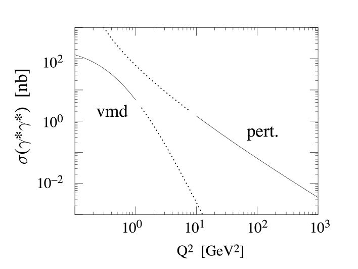
FIG. 10.: $Q^{2}$-behavior of the vector meson dominance and perturbative cross sections in lowest order, with $Q_{A}^{2}=Q_{B}^{2}=Q^{2}$.

The region of intermediate values of $Q^{2}$ in Fig. 10 ($Q$ of the order of $1\ {\mbox{GeV}}$) is where the transition from the soft-scattering regime to the hard-scattering regime is expected to occur. The mechanism through which this happens is not theoretically under control at present, and one may consider trying to estimate the cross section in this region by interpolating between the two curves.

In the next section we will study the prospects for investigating high energy $\gamma^{*}\,\gamma^{*}$ scattering at $e^{+}\,e^{-}$ colliders, and we will discuss which regions in $Q^{2}$ in Fig. 10 can likely be accessed experimentally at LEP200 and a future $e^{+}e^{-}$ collider.

X Numerical results for the electron-positron cross section

The cross section for high energy virtual photon scattering can be measured in $e^{+}\,e^{-}$ collisions in which the outgoing leptons are tagged. The cross section for the electron-positron scattering process is obtained by folding the $\gamma^{*}\,\gamma^{*}$ cross section with the flux of photons from each lepton. Consider the four-fold differential $e^{+}\,e^{-}$ cross section averaged over the angle between the lepton scattering planes, Eq. (5). To get an estimate of the rates available to study BFKL effects in virtual photon scattering at $e^{+}\,e^{-}$ colliders of the present and next generation, we integrate this cross section over a region ${\cal R}$ determined by cuts that we discuss below:

$$\sigma=\int_{{\cal R}}\,{{d\,x_{A}}}\,{{d\,x_{B}}}\,{{d\,Q^{2}_{A}}\over{Q^{2}_{A}}}\,{{d\,Q^{2}_{B}}\over{Q^{2}_{B}}}\,{{Q^{2}_{A}\,Q^{2}_{B}\,d\,\sigma^{(e^{+}e^{-})}}\over{dx_{A}\,dx_{B}\,dQ^{2}_{A}\,dQ^{2}_{B}}}\hskip 11.38092pt.$$ (136)

We choose

i) $Q_{A}>Q_{\rm min}$, $Q_{B}>Q_{\rm min}$, where $Q_{\rm min}$ is a few GeV, in order that the coupling $\alpha_{s}$ be small, and that the process be dominated by the perturbative contribution;

ii) $x_{A}\,x_{B}\,s_{ee}>{\kappa}\,Q_{A}\,Q_{B}$, in order that the high energy approximation be valid. We discuss the parameter ${\kappa}$ below.

Note that, with these criteria, the photon virtualities $Q^{2}$ lie in a range $Q_{\rm min}^{2}<Q^{2}\ll s$ in which the equivalent photon approximation (Eq. (5)) is expected to work fairly well. On one hand, kinematical corrections of order $Q^{2}/s$ are suppressed in this range. On the other hand, contributions of order $m_{e}^{2}/Q^{2}$ to the $e\to e\,\gamma$ splitting process can be neglected.

To choose a value for the parameter ${\kappa}$, we compare the gluon exchange contribution with contributions that are suppressed by a power of $s$ [5, 6]. We consider first the two gluon exchange graph, for which $\sigma\sim s^{0}$ for large $s$. Taking the case $Q_{A}=Q_{B}\equiv Q$, we have from Fig. 4

$$\sigma^{(0)}(s,Q^{2})\,\approx\;{{0.9\times 16\,\;\alpha^{2}\,\alpha_{s}^{2}\,\left(\sum_{q}e^{2}_{q}\right)^{2}}\over{Q^{2}}}\,\left(1+{\cal O}(Q^{2}/s)\right)\hskip 22.76228pt.$$ (137)

Next, we consider the leading order (electromagnetic) contribution to $\gamma^{*}\,\gamma^{*}\to q\,{\bar{q}}$, occurring via quark exchange, for which $\sigma^{(q)}\sim 1/s$. In Appendix B we report results for this subprocess. For $Q_{A}=Q_{B}=Q$ and large enough $s$, the corresponding cross section is well approximated by the formula:

$${\sigma}^{(q)}(s,Q^{2})\,\approx\;{{8\,\pi\,\alpha^{2}\,\sum_{q}e_{q}^{4}\,}\over{s}}\,\left(\ln(s/Q^{2})-1\right)\,\left(1+{\cal O}(Q^{2}/s)\right)\hskip 22.76228pt.$$ (138)

Demanding that the gluon exchange graph give a larger contribution than the quark exchange graph leads to the requirement

$${s\over Q^{2}}\,{1\over{\left(\ln(s/Q^{2})-1\right)}}\,\gtrsim\,\,{1\over\alpha_{s}^{2}}\;\,{{8\,\pi\,\sum_{q}e_{q}^{4}\,}\over{0.9\times 16\,\left(\sum_{q}e^{2}_{q}\right)^{2}}}\,\approx\,{1\over\alpha_{s}^{2}}\hskip 22.76228pt.$$ (139)

For typical perturbative values, $\alpha_{s}\approx 0.2$, we get $s/Q^{2}\gtrsim 10^{2}$. We will therefore use $10^{2}$ as a standard value for ${\kappa}$.

We note that for $s/Q^{2}\gtrsim 10^{2}$, one is surely entitled to drop terms in the gluon exchange graphs that are suppressed by powers of $Q^{2}/s$, as we have done.

We thus compute the integrated rate $\sigma$ in Eq. (136) using the results given in Sec. IV for the photon-photon cross section, and setting the scales in the running coupling and in the high energy logarithms according to the prescriptions discussed in Sec. V. The dependence of $\sigma$ on the lower bound $Q_{\rm min}^{2}$ on the photon virtualities is shown by the “summed” curve in Fig. 11 for the energy of a future $e^{+}e^{-}$ collider. Fig. 12 shows the cross section for the LEP collider at CERN operating at $\sqrt{s}=200\ {\rm GeV}$.

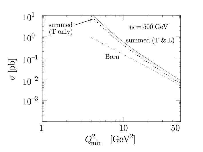
FIG. 11.: The $Q_{\rm min}^{2}$ dependence of the integrated rate $\sigma$, Eq. (136), for $\sqrt{s}=500\ {\rm GeV}$. We take $\kappa=10^{2}$. We set the scales $\mu^{2}$ and $Q^{2}$ according to the prescriptions given in Eqs. (104) and (111). The solid curve represents the full leading log summation, while the dot-dashed curve shows the Born result. The dotted curve shows the contribution to the fully summed result coming from transversely polarized photons.

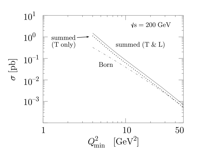
FIG. 12.: Same as in Fig. 11 for $\sqrt{s}=200\ {\rm GeV}$.

The dashed and solid lines in Figs. 11 and 12 correspond to the result of using, respectively, the Born and the summed expressions for the photon-photon cross section. At the values of $\sqrt{s}$ considered in the figures, summation effects enhance the rates significantly in the range of $Q_{\rm min}$ of a few GeV. As $Q_{\rm min}$ increases, lowest order perturbation theory gets closer and closer to the fully summed prediction, as a result of both $\alpha_{s}$ becoming small and the phase space closing up for the high energy logarithms.

In Figs. 11 and 12, we also plot separately the contribution to the cross section from purely transverse photons, that is, the contribution from the term in $\sigma^{(TT)}$ in Eq. (5). We see that this contribution accounts for about three quarters of the full cross section.

For values of the cuts $Q_{\rm min}=2\ {\mbox{GeV}}$, ${\kappa}=10^{2}$, we find

$$\sigma\simeq 1.5\,{\mbox{pb}}\hskip 56.9055pt(\sqrt{s}=200\ {\mbox{GeV}})$$ (140)

at LEP200 energies, and

$$\sigma\simeq 12\,{\mbox{pb}}\hskip 56.9055pt(\sqrt{s}=500\ {\mbox{GeV}})$$ (141)

at the energy of a future collider. These cross sections would give rise to about $750$ events at LEP200 for a value of the luminosity $L=500\,{\mbox{pb}}^{-1}$, and about $6\times 10^{5}$ events at $\sqrt{s}=500\ {\rm GeV}$ for $L=50\,{\mbox{fb}}^{-1}$.

The choice of the cuts that can realistically be implemented is affected by experimental constraints. In particular, the lowest photon virtualities that can be reached are limited by the angular acceptance of the detector, according to the relation $Q^{2}\approx(1-x)E^{2}\,\theta^{2}$, where $E$ is the beam energy, $\theta$ the angle of the tagged lepton, and $x$ is the momentum fraction of the emitted photon. In this situation, the value $Q_{\rm min}=2\ {\mbox{GeV}}$, for which the rates (140), (141) are given, implies detecting leptons scattered through angles down to about $20\ {\mbox{mrad}}$ at LEP200, which is close to the range of the current luminosity monitors at the LEP experiments [23]. For a future 500 GeV collider, $Q_{\rm min}=2\ {\rm GeV}$ corresponds to a minimum angle of about $8\ {\mbox{mrad}}$. It appears that working down to such an angle will be difficult but not impossible [24]. If instead we take $Q_{\rm min}=6\ {\rm GeV}$, the minimum angle is $24\ {\mbox{mrad}}$. Then the cross section is about $2\times 10^{-2}\ {\rm pb}$, corresponding to about $10^{3}$ events.

As stated earlier, the numerical results given above depend on the choice of the scales in $\alpha_{s}$ and in the high energy logarithms that enter the photon-photon cross section. For the calculations described above, we have used the prescriptions given in Sec. V. Different scale choices are possible, and they would affect the predictions at the next-to-leading logarithmic order, which is beyond the present theoretical accuracy. We can use the variation of the results with the scale choices to get an estimate of the uncertainties associated with unknown sub-leading corrections. We can vary the two scales $\mu^{2}$ and $Q^{2}$ (see Eqs. (104), (111)) independently. An illustration of this is reported in Fig. 13. Here we compare the result of Fig. 11 with the curve obtained by multiplying the scale in $\alpha_{s}$ by a factor of $4$, $\mu^{2}\to 4\times\mu^{2}$, and the curve obtained by reducing the scale in the high energy logarithms by a factor of $4$, $Q^{2}\to Q^{2}/4$. The band between these two curves indicates that the uncertainty on the leading logarithmic result is fairly large, and emphasizes the need for improving the accuracy of the calculations at high energy.

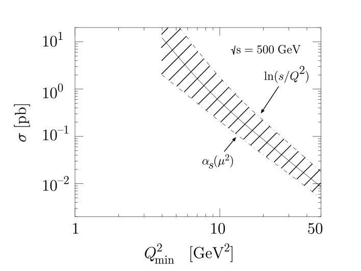
FIG. 13.: Estimate of the uncertainty on the leading logarithmic result for the rate $\sigma$. The solid curve is the summed result shown in Fig. 11. The dot-dashed curves summarize the variation of this prediction as a result of varying the scales in the strong coupling ($\mu^{2}\to 4\mu^{2}$) and the high energy logarithms ($Q^{2}\to Q^{2}/4$).

The plots of the cross section versus $Q_{\rm min}^{2}$ shown in Figs. 11 and 12 illustrate the expected dependence of the photon-photon cross section on the photon virtualities. If we fix $Q_{\rm min}$ we can look at the dependence on the photon-photon c.m. energy $\sqrt{\hat{s}}$. It is useful to use

$$\hat{s}=x_{A}\,x_{B}s$$ (142)

and the photon-photon rapidity

$$y={1\over 2}\,\ln\left(x_{A}\over x_{B}\right)$$ (143)

as variables instead of $x_{A}$ and $x_{B}$. Then we define

$${d\sigma\over d\ln\hat{s}\,dy}\equiv\int_{Q_{\rm min}}^{\hat{s}/(\kappa Q_{\rm min})}dQ_{A}\int_{Q_{\rm min}}^{\hat{s}/(\kappa Q_{A})}dQ_{B}{d\sigma\over d\ln\hat{s}\,dy\,dQ_{A}\,dQ_{B}}$$ (144)

Using Eq. (5), we can write $d\sigma/(d\ln\hat{s}\,dy)$ as

$${d\sigma\over d\ln\hat{s}\,dy} = \left({\alpha\over\pi}\right)^{\!2}x_{A}P^{(T)}_{\gamma/e^{+}}(x_{A})\ x_{B}P^{(T)}_{\gamma/e^{-}}(x_{B})$$ (147)

$$\times\int_{Q_{\rm min}}^{\hat{s}/(\kappa Q_{\rm min})}{dQ_{A}\over Q_{A}}\int_{Q_{\rm min}}^{\hat{s}/(\kappa Q_{A})}{dQ_{B}\over Q_{B}}\ \sigma_{\gamma^{*}\gamma^{*}}^{TT}(\hat{s},Q_{A}^{2},Q_{B}^{2})$$

$$+\cdots\,,$$

where we omit three similar terms. We see that $d\sigma/(d\ln\hat{s}\,dy)$ is very directly related to the $\gamma\,\gamma$ cross section.

We plot ${d\sigma/(d\ln\hat{s}\,dy)}$ at $y=0$ in Fig. 14 for $\sqrt{s}=200\ {\rm GeV}$ and in Fig. 15 for $\sqrt{s}=500\ {\rm GeV}$. Here we choose $Q_{\rm min}^{2}=10\ {\rm GeV}^{2}$ and $\kappa=10^{2}$. In each case, we show a curve for the Born level cross section and another for the full BFKL cross section. We also show the cross section arising from the scattering of (transversely polarized) photons via quark exchange instead of gluon exchange. We see that, with our choice of cuts, quark exchange scattering is suppressed.

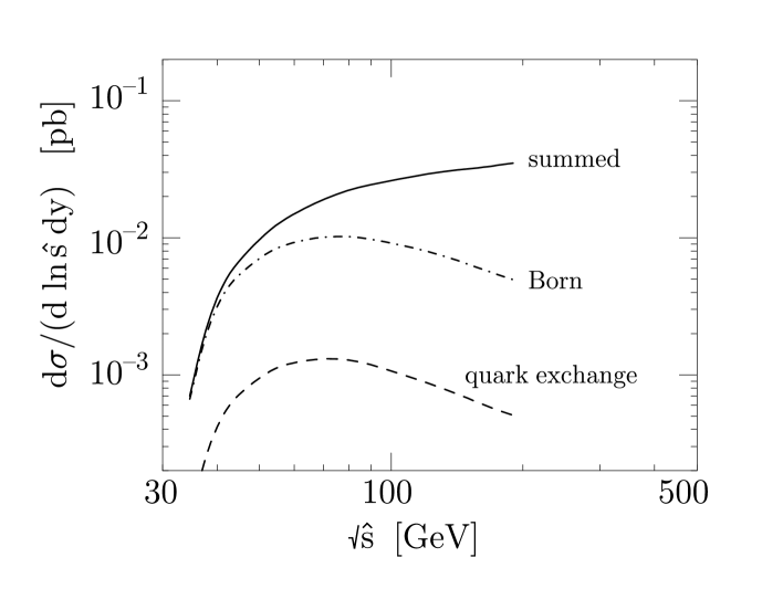
FIG. 14.: The cross section $d\sigma/(d\ln\hat{s}\,dy)$, Eq. (144), at $y=0$ for $\sqrt{s}=200\ {\rm GeV}$. The solid curve is the summed BFKL result. The dot-dashed curve is the Born result. The dashed curve shows the cross section arising from the scattering of (transversely polarized) photons via quark exchange. The cuts are $Q_{\rm min}^{2}=10\ {\rm GeV}^{2}$ and $\kappa=10^{2}$.

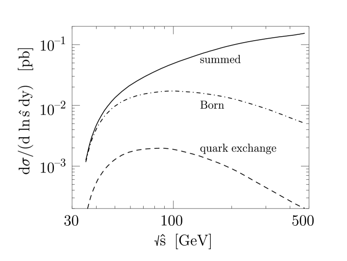
FIG. 15.: Same as in Fig. 14 but for $\sqrt{s}=500\ {\rm GeV}$.

For $\sqrt{\hat{s}}\lesssim 50\ {\rm GeV}$ the cross section shows a strong dependence on the cut $\kappa\,Q_{A}Q_{B}<\hat{s}$. With our choice of $\kappa=100$ and with $Q_{A},Q_{B}>Q_{\rm min}=\sqrt{10}\ {\rm GeV}$, the cross section is forced to vanish for $\sqrt{\hat{s}}<31.6\ {\rm GeV}$. As $\sqrt{\hat{s}}$ increases, the effect of this cut on the $Q_{A}$ and $Q_{B}$ integrations becomes less and less important. Since $\sigma_{\gamma^{*}\gamma^{*}}(\hat{s},Q_{A}^{2},Q_{B}^{2})$ is independent of $\hat{s}$ at Born level, the cross section begins to flatten out as $\sqrt{\hat{s}}$ increases to about $100\ {\rm GeV}$. For larger values of $\sqrt{\hat{s}}$, the Born cross section decreases because of the influence of the photon flux factor $x_{A}P(x_{A})\ x_{B}P(x_{B})=(\hat{s}/s)P([{\hat{s}/s}]^{1/2})^{2}$. For the summed BFKL curve, the growth of $\sigma_{\gamma^{*}\gamma^{*}}(\hat{s},Q_{A}^{2},Q_{B}^{2})$ overcomes the effect of the photon flux factor, so that the cross section rises with $\sqrt{\hat{s}}$.

The curves for $\sqrt{s}=200\ {\rm GeV}$ and $\sqrt{s}=500\ {\rm GeV}$ are similar. The main difference is that at $\sqrt{s}=500\ {\rm GeV}$ there is more available range for $\sqrt{\hat{s}}$.

Our plots are for $y=0$. The available range of $y$ is $|y|<{\scriptstyle{1\over 2}}\,\ln(s/\hat{s})$. Thus the cross section integrated over $y$ goes to zero as $\sqrt{\hat{s}}\to\sqrt{s}$.

We see from the results presented above that at a future $e^{+}e^{-}$ collider it should be possible to probe the effects of pomeron exchange in a range of $Q^{2}$ where summed perturbation theory applies. One should be able to investigate this region in detail by varying $Q_{A}$, $Q_{B}$ and ${\hat{s}}=x_{A}\,x_{B}\,s_{ee}$ independently. At LEP200 such studies appear to be more problematic mainly because of limitations in luminosity. Even with a modest luminosity, however, one can access the region of relatively low $Q^{2}$ in the graph of Fig. 10 if one can get down to small enough angles. This would allow one to examine experimentally the transition between soft and hard scattering.

We now move on to the angular distribution for the $e^{+}\,e^{-}$ scattering cross section, and consider the asymmetries $A_{1}$, $A_{2}$ introduced in Eq. (1). As pointed out in Sec. III, $A_{1}$ is zero at leading order. On the other hand, $A_{2}$ is given by an equivalent-photon formula in terms of the asymmetry ${\cal A}$ for the $\gamma^{*}\,\gamma^{*}$ scattering process discussed in Sec. IV B. This reads

$$A_{2}\,{{Q^{2}_{A}\,Q^{2}_{B}\,d\,\sigma^{(e^{+}e^{-})}}\over{dx_{A}\,dx_{B}\,dQ^{2}_{A}\,dQ^{2}_{B}}}$$ (148)

$$=\left({\alpha\over{2\,\pi}}\right)^{2}\,{{1-x_{A}}\over x_{A}}\,{{1-x_{B}}\over x_{B}}\,{\cal A}_{\gamma^{*}\,\gamma^{*}}(x_{A}\,x_{B}\,s,Q^{2}_{A},Q^{2}_{B}){\overline{\sigma}}_{\gamma^{*}\,\gamma^{*}}(x_{A}\,x_{B}\,s,Q^{2}_{A},Q^{2}_{B})\,\;\;\;,$$ (149)

with ${\cal A}$ and ${\overline{\sigma}}$ being given in Eqs. (95), (85).

We can use the same cuts discussed earlier in this section to integrate Eq. (148), and thus define

$${\tilde{A}}_{2}={1\over\sigma}\,\int_{{\cal R}}\,{{d\,x_{A}}}\,{{d\,x_{B}}}\,{{d\,Q^{2}_{A}}\over{Q^{2}_{A}}}\,{{d\,Q^{2}_{B}}\over{Q^{2}_{B}}}\,A_{2}\,{{Q^{2}_{A}\,Q^{2}_{B}\,d\,\sigma^{(e^{+}e^{-})}}\over{dx_{A}\,dx_{B}\,dQ^{2}_{A}\,dQ^{2}_{B}}}\hskip 11.38092pt,$$ (150)

where $\sigma$ is the integrated rate in Eq. (136). Performing the integral numerically, we find that the asymmetry ${\tilde{A}}_{2}$ is very small. As noted in Sec. IV, the role of the summed BFKL terms is that of reducing the magnitude of the asymmetry with respect to the Born order result. At a 500 GeV collider, in the range of the angular and energy cuts previously described, we find ${\tilde{A}}_{2}\simeq 10^{-3}$. We observe that spin effects in photon-photon scattering at high energies are interesting, but the predicted asymmetries are either zero or small.

XI Conclusions

Understanding the behavior of high energy hadron reactions from a fundamental perspective within QCD is an important goal of particle physics. As we have shown in this paper, virtual photon scattering $\gamma^{*}(Q_{A}^{2})+\gamma^{*}(Q_{B}^{2})\to hadrons$ at high energies, $s>>Q_{A}^{2},Q_{B}^{2}$, provides a remarkable window into pomeron physics. The total cross section can be studied as a function of the space-like mass of each incident projectile. Most importantly, the process can be investigated in the regime where the photons both have large virtuality, so that one can use the framework of perturbative QCD.

Compared to tests of the QCD pomeron behavior based on deeply inelastic structure functions, the measurement of the total cross section for sufficiently off-shell photons is free from the long-distance ambiguities related to the structure of the hadronic target. On the other hand, unlike tests based on associated jet production in lepton-hadron or hadron-hadron collisions, the $\gamma^{*}\gamma^{*}$ measurement is fully inclusive and therefore it does not depend on specifying the details of the final state.

The scattering of highly virtual photons can be described as the interaction of two incident color singlet $q\bar{q}$ pairs of small transverse size interacting through multiple gluon exchange. We have studied this reaction both in the Born approximation (corresponding to two-gluon exchange) and also with the inclusion of the higher-order summation encompassed by the BFKL equation. The cross section at high energies and large virtuality takes a factorized form in transverse coordinates. However, it does not factorize simply into separate functions of $Q_{A}^{2}$ and $Q_{B}^{2}$, which reflects the cut structure of the BFKL pomeron in the complex angular momentum plane. We have also examined the background contribution from quark exchange, a process which is power-law suppressed at high energy.

According to this analysis, the $\gamma^{*}\gamma^{*}$ cross section falls off at high virtuality only as $1/Q^{2}$, where $Q^{2}\sim{\mbox{max}}\{Q_{A}^{2},Q_{B}^{2}\}$. The rate for sensitive tagged-lepton experiments at high energy $e^{\pm}e^{-}$ or $\mu^{\pm}\mu^{-}$ colliders is thus not negligible. In particular it appears that the main features of the perturbative QCD predictions, such as the energy dependence, the factorization properties of the cross section, the scaling laws in $Q_{A}^{2}$, $Q_{B}^{2}$, as well as the polarization and azimuthal correlations can be tested in detail at a high-energy and high-luminosity next linear collider. We have also found that an interesting first look at virtual photon scattering can be obtained from the tagged lepton events measured in the luminosity monitors of present experiments at LEP200.

More precisely, we estimate that, in the region of photon virtualities where summed perturbation theory is expected to apply, there should be several hundred events at LEP200, and about $10^{5}$ events at a future 500 GeV collider with an integrated luminosity of $50\ {\rm fb}^{-1}$. We also find that the enhancement due to BFKL pomeron terms over the Born cross section is sizable, and should be visible particularly in the ${\hat{s}}$-distribution of the cross section, with ${\hat{s}}=x_{A}\,x_{B}\,s_{ee}$.

The dependence of the cross section on the photon virtualities $Q_{A}$ and $Q_{B}$ is perturbative, and can be predicted in the framework of the BFKL equation. These predictions can be tested by measuring the angles of the recoil leptons. Both the case in which the two photon virtualities are varied together ($Q_{A}\sim Q_{B}$) and the case in which they are kept far apart ($Q_{A}\gg Q_{B}$) are of interest. In the second case one gets to observe the structure function of a virtual photon at small Bjorken-$x$.

The spin structure is rich, but hard to observe. Most of the observable cross section comes from the scattering of two transversely polarized photons. For this part of the cross section, there is an asymmetry in the angular distribution of the outgoing leptons, but this asymmetry is less than $1\%$.

In the region of low photon virtualities ($Q_{A},\,Q_{B}$ smaller than a few GeV), the photon-photon cross section becomes dominated by soft interactions. Here one cannot use a perturbative analysis. On the other hand, one may explore experimentally at what scales the breakdown of the perturbative result occurs, and how this is connected to the onset of the phenomenological “soft-pomeron” behavior.

The theory that is available at present is leading logarithmic and therefore is affected by rather large uncertainties. These uncertainties can be parametrized in terms of two mass scales, the transverse scale that controls the running coupling and the longitudinal scale associated with the high energy logarithms. A next-to-leading logarithmic calculation would help determine these scales. Such a calculation could make the theoretical predictions much more precise. At the largest values of $\hat{s}$, new effects related to unitarity and diffusion may become important. If so, an improved theory that deals with these effects would be testable at a future $e^{+}e^{-}$ collider.

A The Born order calculation

We start with the expression (12) for the amplitude corresponding to the graph in Fig. 2. The overall charge factor in Eq. (12) is

$$\sum_{a,b}\,g_{s}^{4}\,e^{2}_{a}\,e^{2}_{b}\,e^{4}\,{\mbox{\rm Tr}}\left(t^{r}t^{s}\right)\,{\mbox{\rm Tr}}\left(t^{r}t^{s}\right)=32\,\alpha^{2}\,\alpha_{s}^{2}\,\left(\sum_{q}e^{2}_{q}\right)^{2}\,(2\,\pi)^{4}\;\;\;,$$ (A1)

where we have used the color trace ${\mbox{\rm Tr}}\left(t^{r}t^{s}\right)=(1/2)\delta^{rs}$.

We use the mass shell constraints on the final quarks, $p_{A}$ and $p_{B}$, to eliminate the integrals over their “$-$” and “$+$” components, respectively, thus obtaining

$$\int{{d^{4}p_{A}}\over{(2\,\pi)^{4}}}\;2\,\pi\,\delta_{+}\!\left(p_{A}^{2}\right)\to\int{{d\,z_{A}}\over{2\,z_{A}}}\,d^{2}\,{{\bf p}}_{A}\,(2\,\pi)^{-3}\;\;,\;\;\;z_{A}^{\prime}={{{\bf p}}_{A}^{2}\over{2\;z_{A}\;q^{+}_{A}q^{-}_{B}}}\;\;,$$ (A2)

$$\int{{d^{4}p_{B}}\over{(2\,\pi)^{4}}}\;2\,\pi\,\delta_{+}\!\left(p_{B}^{2}\right)\to\int{{d\,z_{B}}\over{2\,z_{B}}}\,d^{2}\,{{\bf p}}_{B}\,(2\,\pi)^{-3}\;\;,\;\;\;z_{B}^{\prime}={{{\bf p}}_{B}^{2}\over{2\;z_{B}\;q^{+}_{A}q^{-}_{B}}}\;\;.$$ (A3)

We use the mass shell constraints on the antiquarks to eliminate the integrals over the “$-$” and “$+$” components of the exchanged momentum $k$, as follows:

$$\int{{d\,k^{-}}\over{2\,\pi}}\;2\,\pi\,\delta_{+}\!\left((q_{A}-p_{A}-k)^{2}\right)\to{1\over{2\;(1-z_{A})\;q^{+}_{A}}}\;\;,\,$$ (A5)

$$k^{-}\simeq-{1\over{2\,q_{A}^{+}}}\,\left(Q_{A}^{2}+{{{{\bf p}}_{A}^{2}}\over z_{A}}+{{({{\bf p}}_{A}+{{\bf k}})^{2}}\over{1-z_{A}}}\right)\;\;\;,$$

$$\int{{d\,k^{+}}\over{2\,\pi}}\;2\,\pi\,\delta_{+}\!\left((q_{B}-p_{B}+k)^{2}\right)\to{1\over{2\;(1-z_{B})\;q^{-}_{B}}}\;\;,$$ (A6)

$$k^{+}\simeq{1\over{2\,q_{B}^{-}}}\,\left(Q_{B}^{2}+{{{{\bf p}}_{B}^{2}}\over z_{B}}+{{({{\bf p}}_{B}-{{\bf k}})^{2}}\over{1-z_{B}}}\right)\;\;\;.$$ (A7)

Note that in Eqs. (A5), (A6) we have neglected terms of order $k^{+}/\sqrt{s}$ and $k^{-}/\sqrt{s}$ with respect to unity, consistently with the high energy approximation.

Eq. (12) can then be rewritten as

$${|{\cal M}|}^{2}=32\,\alpha^{2}\,\alpha_{s}^{2}\,\left(\sum_{q}e^{2}_{q}\right)^{2}\,(2\,\pi)^{4}\,\int\;{{d^{2}\,{\bf k}}\over{(2\,\pi)^{2}}}\;{{d^{2}\,{{\bf p}}_{A}}\over{(2\,\pi)^{2}}}\;{{d^{2}\,{{\bf p}}_{B}}\over{(2\,\pi)^{2}}}$$ (A8)

$$\times\,\int_{0}^{1}{1\over{2\,\pi}}\;{{d\,z_{A}}\over{2\,z_{A}\,(1-z_{A})}}\int_{0}^{1}{1\over{2\,\pi}}\;{{d\,z_{B}}\over{2\,z_{B}\,(1-z_{B})}}\;{1\over{2\,s}}\,{1\over{(k^{2})^{2}}}\,$$ (A9)

$$\times\,{{{\mbox{\rm Tr}}\left[\,{\hbox to0.0pt{/\hss}p}_{A}\,\gamma_{\alpha}\,({\hbox to0.0pt{/\hss}p}_{A}+\hbox to0.0pt{/\hss}k)\,{\hbox to0.0pt{/\hss}\varepsilon}_{A}\,({\hbox to0.0pt{/\hss}q}_{A}-{\hbox to0.0pt{/\hss}p}_{A}-\hbox to0.0pt{/\hss}k)\,\gamma_{\beta}\,({\hbox to0.0pt{/\hss}p}_{A}-{\hbox to0.0pt{/\hss}q}_{A})\,{\hbox to0.0pt{/\hss}\varepsilon}_{A}\right]}\over{\left((p_{A}+k)^{2}+i\,\varepsilon\right)\left((p_{A}-q_{A})^{2}-i\,\varepsilon\right)}}\,$$ (A10)

$$\times\,{{{\mbox{\rm Tr}}\left[\,{\hbox to0.0pt{/\hss}p}_{B}\,\gamma^{\alpha}\,({\hbox to0.0pt{/\hss}p}_{B}-\hbox to0.0pt{/\hss}k)\,{\hbox to0.0pt{/\hss}\varepsilon}_{B}\,({\hbox to0.0pt{/\hss}q}_{B}-{\hbox to0.0pt{/\hss}p}_{B}+\hbox to0.0pt{/\hss}k)\,\gamma^{\beta}\,({\hbox to0.0pt{/\hss}p}_{B}-{\hbox to0.0pt{/\hss}q}_{B})\,{\hbox to0.0pt{/\hss}\varepsilon}_{B}\right]}\over{\left((p_{B}-k)^{2}+i\,\varepsilon\right)\left((p_{B}-q_{B})^{2}-i\,\varepsilon\right)}}\;\;.$$ (A11)

We now re-express the denominators and numerators of the amplitude (12) in the high energy limit. With the neglect of terms of order $k^{+}/\sqrt{s}$ and $k^{-}/\sqrt{s}$, the denominators take the form

$$(p_{A}+k)^{2}\simeq-{1\over{1-z_{A}}}\,\left(z_{A}\,(1-z_{A})\,Q^{2}_{A}+({{\bf p}}_{A}+{{\bf k}})^{2}\right)\,\;,\;\;\;$$ (A12)

$$(p_{A}-q_{A})^{2}\simeq-{1\over z_{A}}\,\left(z_{A}\,(1-z_{A})\,Q^{2}_{A}+{{\bf p}}_{A}^{2}\right)\;\;\;,$$ (A13)

and analogously

$$(p_{B}-k)^{2}\simeq-{1\over{1-z_{B}}}\,\left(z_{B}\,(1-z_{B})\,Q^{2}_{B}+({{\bf p}}_{B}-{{\bf k}})^{2}\right)\,\;,\;\;\;$$ (A14)

$$(p_{B}-q_{B})^{2}\simeq-{1\over z_{B}}\,\left(z_{B}\,(1-z_{B})\,Q^{2}_{B}+{{\bf p}}_{B}^{2}\right)\;\;\;.$$ (A15)

In the numerator, light-cone gluon polarizations are dominant at high energy, and therefore we are led to calculate the product of traces

$$T_{A}^{++}\,T_{B}^{--}$$ (A16)

$$={\mbox{\rm Tr}}\left[\,{\hbox to0.0pt{/\hss}p}_{A}\,\gamma^{+}\,({\hbox to0.0pt{/\hss}p}_{A}+\hbox to0.0pt{/\hss}k)\,{\hbox to0.0pt{/\hss}\varepsilon}_{A}\,({\hbox to0.0pt{/\hss}q}_{A}-{\hbox to0.0pt{/\hss}p}_{A}-\hbox to0.0pt{/\hss}k)\,\gamma^{+}\,({\hbox to0.0pt{/\hss}p}_{A}-{\hbox to0.0pt{/\hss}q}_{A})\,{\hbox to0.0pt{/\hss}\varepsilon}_{A}\right]\;$$ (A17)

$$\times\,{\mbox{\rm Tr}}\left[\,{\hbox to0.0pt{/\hss}p}_{B}\,\gamma^{-}\,({\hbox to0.0pt{/\hss}p}_{B}-\hbox to0.0pt{/\hss}k)\,{\hbox to0.0pt{/\hss}\varepsilon}_{B}\,({\hbox to0.0pt{/\hss}q}_{B}-{\hbox to0.0pt{/\hss}p}_{B}+\hbox to0.0pt{/\hss}k)\,\gamma^{-}\,({\hbox to0.0pt{/\hss}p}_{B}-{\hbox to0.0pt{/\hss}q}_{B})\,{\hbox to0.0pt{/\hss}\varepsilon}_{B}\right]\;.$$ (A18)

The result reads

$$T_{A}^{++}\,T_{B}^{--}$$ (A19)

$$= 8\,(q_{A}^{+})^{2}\,\left(4z_{A}(1-z_{A}){\bf{\varepsilon}}_{A}\cdot{{\bf p}}_{A}\;{\bf{\varepsilon}}_{A}\cdot({{\bf p}}_{A}+{\bf k})-{{\bf p}}_{A}\cdot({{\bf p}}_{A}+{\bf k})\right)\,$$ (A20)

$$\times 8\,(q_{B}^{-})^{2}\,\left(4z_{B}(1-z_{B}){\bf{\varepsilon}}_{B}\cdot{{\bf p}}_{B}\;{\bf{\varepsilon}}_{B}\cdot({{\bf p}}_{B}-{\bf k})-{{\bf p}}_{B}\cdot({{\bf p}}_{B}-{\bf k})\right)\;\;\;.$$ (A21)

Substituting Eqs. (A12)-(A15) and (A19) in Eq. (A8), we obtain the expression (16) for the amplitude corresponding to the graph in Fig. 2.

The total cross section is arrived at by adding the contributions from the other graphs according to the replacements described in the text below Eq. (16), and dividing by $2\,s$. The result reads

$$\sigma^{(0)}_{\gamma^{*}\,\gamma^{*}}=128\,\alpha^{2}\,\alpha_{s}^{2}\,\left(\sum_{q}e^{2}_{q}\right)^{2}\,(2\,\pi)^{2}\,\int\;{{d^{2}\,{\bf k}}\over{(2\,\pi)^{2}}}\;{{d^{2}\,{{\bf p}}_{A}}\over{(2\,\pi)^{2}}}\;{{d^{2}\,{{\bf p}}_{B}}\over{(2\,\pi)^{2}}}\;\int_{0}^{1}{d\,z_{A}}\int_{0}^{1}{d\,z_{B}}\,{1\over{({{\bf k}}^{2})^{2}}}$$ (A22)

$$\times\,\left\{{{\left[4z_{A}(1-z_{A}){\bf{\varepsilon}}_{A}\cdot{{\bf p}}_{A}\;{\bf{\varepsilon}}_{A}\cdot({{\bf p}}_{A}+{\bf k})-{{\bf p}}_{A}\cdot({{\bf p}}_{A}+{\bf k})\right]}\over{\left[z_{A}\,(1-z_{A})\,Q^{2}_{A}+({{\bf p}}_{A}+{{\bf k}})^{2}\right]\,\left[z_{A}\,(1-z_{A})\,Q^{2}_{A}+{{\bf p}}_{A}^{2}\right]}}\right.$$ (A24)

$$\hskip 28.45274pt\left.-{{\left[4z_{A}(1-z_{A})({\bf{\varepsilon}}_{A}\cdot{{\bf p}}_{A})^{2}\;-{{\bf p}}_{A}^{2}\right]}\over{\left[z_{A}\,(1-z_{A})\,Q^{2}_{A}+{{\bf p}}_{A}^{2}\right]^{2}}}\right\}$$

$$\times\,\left\{{{\left[4z_{B}(1-z_{B}){\bf{\varepsilon}}_{B}\cdot{{\bf p}}_{B}\;{\bf{\varepsilon}}_{B}\cdot({{\bf p}}_{B}-{\bf k})-{{\bf p}}_{B}\cdot({{\bf p}}_{B}-{\bf k})\right]}\over{\left[z_{B}\,(1-z_{B})\,Q^{2}_{B}+({{\bf p}}_{B}-{{\bf k}})^{2}\right]\,\left[z_{B}\,(1-z_{B})\,Q^{2}_{B}+{{\bf p}}_{B}^{2}\right]}}\right.$$ (A26)

$$\hskip 28.45274pt\left.-{{\left[4z_{B}(1-z_{B})({\bf{\varepsilon}}_{B}\cdot{{\bf p}}_{B})^{2}\;-{{\bf p}}_{B}^{2}\right]}\over{\left[z_{B}\,(1-z_{B})\,Q^{2}_{B}+{{\bf p}}_{B}^{2}\right]^{2}}}\right\}.$$

This coincides with Eq. (22) in the text once the explicit expression (23) for $G$ is used.

Using Eqs. (A8)-(A16), the tensor ${\cal G}^{\,\mu\,\nu\,}({\bf k};Q^{2})$ introduced in Eq. (49) takes the form

$${\cal G}^{\,\mu\,\nu\,}({\bf k};Q^{2})={\alpha\,\alpha_{s}\over 4(q_{A}^{+})^{2}}\,\left(\sum_{q}e^{2}_{q}\right)\,\int\;{{d^{2}\,{{\bf p}}}\over{\pi}}\;\int_{0}^{1}\,{d\,z}\,$$ (A27)

$$\times\,\left\{{{{\mbox{\rm Tr}}\left[\,{\hbox to0.0pt{/\hss}p}\,\gamma^{+}\,({\hbox to0.0pt{/\hss}p}+\hbox to0.0pt{/\hss}k)\,\gamma^{\mu}\,({\hbox to0.0pt{/\hss}q}-{\hbox to0.0pt{/\hss}p}-\hbox to0.0pt{/\hss}k)\,\gamma^{+}\,({\hbox to0.0pt{/\hss}p}-{\hbox to0.0pt{/\hss}q})\,\gamma^{\nu}\right]}\over{\left[({{\bf p}}+{{\bf k}})^{2}+z\,(1-z)\,Q^{2}\right]\,\left[{{\bf p}}^{2}+z\,(1-z)\,Q^{2}\right]}}+\,symm.\,\right\}\;\;\;,$$ (A28)

where the additive symmetric terms are obtained from the replacements given in Sec. II.

B Comparison with the cross section from quark exchange

The gluon exchange diagrams discussed in the text provide the dominant contribution to the photon-photon cross section in the high energy limit. They give rise to constant (in Born order) or logarithmic (in higher orders) terms at large $s$ in the cross section. This appendix is concerned with quark exchange contributions, which vanish in the large energy limit. We examine quark exchange in order to estimate the energy at which gluon exchange becomes dominant.

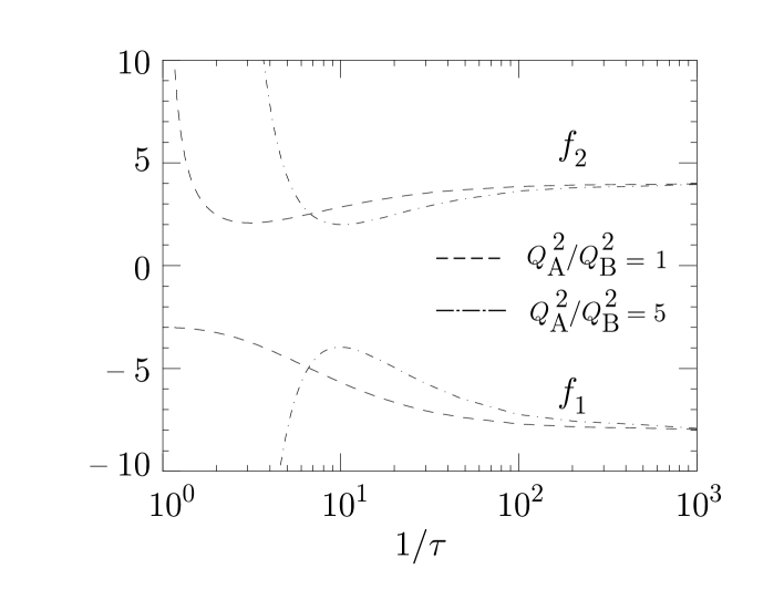
FIG. 16.: The $\tau$-dependence of the functions $f_{1}$ and $f_{2}$ that enter the leading order expression for ${\sigma}^{(q)}$, Eq. (B4). We report $f_{1}$ and $f_{2}$ for two different values of $Q_{A}^{2}/Q_{B}^{2}$.

The leading-order term of quark-exchange type comes from the purely electromagnetic process

$$\gamma^{*}(q_{A})+\gamma^{*}(q_{B})\to q(p)+{\bar{q}}({\bar{p}})\;\;\;.$$ (B1)

This contribution is suppressed by a power of $s$ at high energies, $\sigma^{(q)}\sim 1/s$. To express the cross section for this process, we parametrize the incoming photon momenta as in Eq. (8), and introduce the variables

$$\xi_{A}={{Q_{A}^{2}}\over{2\,q^{+}_{A}\,q^{-}_{B}}}\hskip 19.91684pt,\hskip 28.45274pt\xi_{B}={{Q_{B}^{2}}\over{2\,q^{+}_{A}\,q^{-}_{B}}}\hskip 28.45274pt,$$ (B2)

in terms of which the total energy $s$ has the expression

$$s=2\,q^{+}_{A}\,q^{-}_{B}\,\;\;(1-\xi_{A})\,(1-\xi_{B})\hskip 28.45274pt.$$ (B3)

In the high energy region one has $\xi_{A},\,\xi_{B}\ll 1$, and $s\sim 2\,q^{+}_{A}\,q^{-}_{B}$ as in Eq. (9).

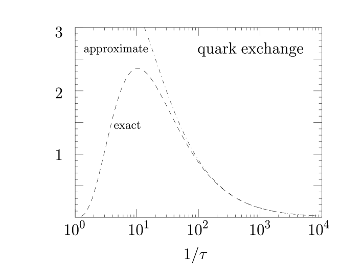
FIG. 17.: The $\tau$-dependence of the quark-exchange contribution to the $\gamma^{*}\gamma^{*}$ cross section in leading order. We take $Q_{A}=Q_{B}$, and we plot the rescaled cross section $Q_{A}\,Q_{B}\,\sigma^{(q)}/\left(\alpha^{2}\,(\sum_{q}e_{q}^{4})\right)$. The dashed curve is the exact expression, Eq. (B4), while the dot-dashed curve is the expression approximated for high energies, Eq. (B5).

The cross section for the process (B1) to order $\alpha^{2}$, averaged over the transverse photon polarizations, has the form

$${\sigma}^{(q)}={{2\,\pi\,\alpha^{2}\,\sum_{q}e_{q}^{4}\,}\over{Q_{A}\,Q_{B}}}{{\sqrt{\xi_{A}\,\xi_{B}}}\over{2\,(1-\xi_{A}\,\xi_{B})}}\left[{{f_{1}}}+{{f_{2}\,\ln\left(1/(\xi_{A}\,\xi_{B})\right)}}\right]\hskip 22.76228pt,$$ (B4)

where $f_{1}$ and $f_{2}$ are rational functions of $\xi_{A},\xi_{B}$, and are plotted in Fig. 16 versus the variable $\tau=\sqrt{\xi_{A}\,\xi_{B}}$ for different values of the ratio $\rho=\xi_{A}/\xi_{B}$.

The $\tau$-dependence of the cross section (B4) is reported in Fig. 17 for the case of equal virtualities. The cross section vanishes at the kinematic threshold $\tau=1$, it has a maximum around $\tau\sim 10^{-1}$, then it falls off and vanishes for $\tau\to 0$ (corresponding to high energy) like $\tau\,\ln\tau$, according to the asymptotic formula

$${\sigma}^{(q)}\simeq{{2\,\pi\,\alpha^{2}\,\sum_{q}e_{q}^{4}\,}\over{Q_{A}\,Q_{B}}}\,4\,\tau\,\left(\ln(1/\tau)-1\right)\hskip 14.22636pt,\hskip 22.76228pt\tau\ll 1\hskip 22.76228pt.$$ (B5)

The power suppression with $\tau$ at small $\tau$ is the one expected from the exchange of a spin-$1/2$ line in the $t$-channel. The logarithmic enhancement is associated with the integration over the region of small angles at the splitting vertex $\gamma^{*}\to q\,{\bar{q}}$ in the limit of small photon virtuality. The behavior of the cross section is qualitatively the same in the case of unequal virtualities.

REFERENCES

[1]
L.N. Lipatov,
Sov. J. Nucl. Phys. 23, 338 (1976);
E.A. Kuraev, L.N. Lipatov and V.S. Fadin,
Sov. Phys. JETP 45, 199 (1977) ;
I. Balitskii and L.N. Lipatov,
Sov. J. Nucl. Phys. 28, 822 (1978).
[2]
H. Abramowicz, plenary talk at ICHEP96 (Warsaw, July 1996),
in Proceedings of the
XXVIII International
Conference on High Energy Physics,
eds. Z. Ajduk and A.K. Wroblewski, World Scientific, p.53.
[3]
D0 Collaboration, Phys. Rev. Lett. 77, 595 (1996).
[4]
S.J. Brodsky, talk at Workshop on High Energy Colliders,
Brookhaven National Laboratory, May 1996.
[5]
F. Hautmann, talk at ICHEP96 (Warsaw, July 1996),
preprint OITS 613/96,
in Proceedings of the
XXVIII International Conference on High Energy Physics,
eds. Z. Ajduk and A.K. Wroblewski, World Scientific, p.705.
[6]
S.J. Brodsky, F. Hautmann and D.E. Soper, Phys. Rev. Lett. 78, 803 (1997).
[7]
P. Aurenche, G.A. Schuler et al., Report
on “ Physics” in Proceedings of the Workshop
“Physics at LEP2”, eds. G. Altarelli,
T. Sjöstrand and F. Zwirner, CERN 1996-01, Vol.1, p.291.
[8]
A.H. Mueller, Nucl. Phys. B415, 373 (1994);
A.H. Mueller and B. Patel,
ibid.B425, 471 (1994).
[9]
I. Balitskii, Nucl. Phys. B463, 99 (1996).
[10]
J. Bartels, A. De Roeck and H. Lotter,
Phys. Lett. B 389, 742 (1996).
[12]
F.E. Low, Phys. Rev. D 12, 163 (1975);
S. Nussinov, Phys. Rev. Lett. 34, 1286 (1975),
Phys. Rev. D 14, 246 (1976);
J.F. Gunion and D.E. Soper,
ibid.15, 2617(1977).
[13]
J.D. Bjorken, J. Kogut and
D.E. Soper, Phys. Rev. D 3, 1382 (1971).
[14]
J.D. Bjorken and J. Kogut, Phys. Rev. D 8, 1341 (1973).
[15]
L.L. Frankfurt and M. Strikman, Phys. Rep. 160,
235 (1988).
[16]
S. Catani, M. Ciafaloni and F. Hautmann,
Phys. Lett. B 242, 97 (1990),
Nucl. Phys. B366, 135 (1991);
J.C. Collins and R.K. Ellis,
ibid.B360, 3 (1991).
[17]
G.P. Lepage and P.B. Mackenzie,
Phys. Rev. D 48, 2250 (1993);
S.J. Brodsky, G.P. Lepage and P.B. Mackenzie,
ibid.28, 228 (1983).
[18]
J.D. Bjorken, preprint SLAC-PUB-7341, presented
at Snowmass 1996 Summer Study
on New Directions for High Energy Physics,
e-print archive hep-ph/9610516.
[19]
J. Bartels and H. Lotter, Phys. Lett. B 309, 400 (1993).
[20]
A.H. Mueller, Nucl. Phys. B437, 107 (1995).
[21]
G.A. Schuler and T. Sjöstrand,
Zeit. Phys. C 68, 607 (1995),
Phys. Lett. B 376, 193 (1996);
M. Glück, E. Reya and M. Stratmann,
Phys. Rev. D 51, 3220 (1995).
[22]
P.D.B. Collins, An introduction to
Regge theory and high energy physics, Cambridge University
Press, Cambridge, 1977.
[23]
OPAL Collaboration, contributed paper pa03-007
at ICHEP96 (Warsaw, July 1996);
J.A. Lauber (OPAL),
in Proceedings of the
XXVIII International Conference on High Energy Physics,
eds. Z. Ajduk and A.K. Wroblewski, World Scientific, p.725.
[24]
S. Kuhlman et al., Physics and Technology of the Next Linear
Collider, Snowmass 1996 Report, e-print archive hep-ex/9605011.