Abstract

I discuss the operator expansion for diffractive high-energy scattering and present the non-linear evolution equation for the relevant Wilson-line operators which describes both the propagator of the BFKL pomeron and the three-pomeron vertex.

Semihard diffractive processes are of special interest since they provide us with valuable information about the non-linear dynamics of the pomerons. (For review of the experimental situation, see ref. [1]). In a recent paper[2] I suggested the operator expansion (OPE) for high-energy amplitudes. It turns out that the small-$x$ behavior of structure functions of DIS is governed by the evolution of Wilson-line operators with respect to the deviation of the supporting lines from the light cone. In this paper, I generalize this approach to diffractive high-energy scattering. In particular, I obtain the cross section of the diffractive dissociation of the virtual photon in the triple Regge limit $s\gg M^{2}\gg Q^{2}$ as a result of the evolution of the relevant Wilson-line operators.

OPE for high-energy amplitudes

First, let me remind the OPE for high-energy amplitudes derived in [2]. Consider the amplitude of forward $\gamma^{*}\gamma^{*}$-scattering at small $x_{B}={Q^{2}\over s}$. In the target frame, the virtual photon splits into $q\bar{q}$ pair which approaches the nucleon at high speed. Due to the high speed the classical trajectories of the quarks are straight lines collinear to the momentum of the incoming photon $q$. The corresponding operator expansion switched between nucleon states has the form [2]:

$$\int\!d^{4}xe^{iq\cdot x}\langle p|T\{j_{\mu}(x)j_{\nu}(0)\}|p\rangle=\int d^{2}x_{\perp}I_{\mu\nu}(x_{\perp})\langle p|\mathop{\rm Tr}\{\hat{U}(x_{\perp})\hat{U^{\dagger}}(0)\}|p\rangle,$$ (1)

where $I_{\mu\nu}(x_{\perp})$ is a certain numerical function of the transverse separation of quarks $x_{\perp}$ and virtuality of the photon $Q^{2}=-q^{2}$. The relevant operators $U(U^{\dagger})$ are gauge factors ordered along the classical trajectories which are almost light-like lines stretching from minus to plus infinity:

$$U(z_{\perp})=P\exp\left(i\int_{-\infty}^{\infty}due^{\mu}A_{\mu}(ue+z_{\perp})\right)$$ (2)

where $e$ is collinear to $q$ and $z_{\perp}$ is the transverse position of the Wilson line.

It turns out that the small-$x$ behavior of structure functions is governed by the evolution of these operators with respect to the deviation of the Wilson lines from the light cone; this deviation serves as a kind of “renormalization point” for these operators. At infinite energy, the vector $e$ is light-like and the corresponding matrix elements of the operators (2) have a logarithmic divergence in longitudinal momenta. To regularize it , we consider operators corresponding to large but finite velocity and take $e_{\zeta}=e_{1}~{}+~{}\zeta e_{2}$ where $e_{1}=(q-\frac{q^{2}}{2pq}p)$ and $e_{2}=p$ are the lightlike vectors close to the directions of the colliding particles. Now, instead of studying the energy-dependence of the physical amplitude we must investigate the dependence of the operators (2) on the slope $\zeta$. Large energies mean small $\zeta$ and we can sum up logarithms of $\zeta$ instead of logarithms of $s$ (At present, we can do it only in the leading logarithmic approximation (LLA) $\alpha_{s}\ll 1$, $\alpha_{s}\ln{s\over m^{2}}\sim 1$). The equation governing the dependense of $U$ on $\zeta$ has the form [2]:

$$\zeta\frac{d}{d\zeta}{\cal U}(x_{\perp},y_{\perp})={3\alpha_{s}\over 2\pi^{2}}\int dz_{\perp}{(x_{\perp}-y_{\perp})^{2}\over(x_{\perp}-z_{\perp})^{2}(z_{\perp}-y_{\perp})^{2}}$$ (3)

$$\left\{{\cal U}(x_{\perp},z_{\perp})+{\cal U}(z_{\perp},y_{\perp})-{\cal U}(x_{\perp},y_{\perp})+{\cal U}(x_{\perp},z_{\perp}){\cal U}(z_{\perp},y_{\perp})\right\}$$ (4)

where ${\cal U}(x_{\perp},y_{\perp})\stackrel{{\scriptstyle\rm def}}{{\equiv}}{1\over 3}\mathop{\rm Tr}\{U(x_{\perp})U^{\dagger}(y_{\perp})\}-1$. The first three linear terms in braces in the r.h.s. of eq. (4)) reproduces the BFKL pomeron[3] while the quadratic term will give us the three-pomeron vertex as we shall see below. The solution of the linearized evolution equation is especially simple in the case of zero momentum transfer (e.g. for the total cross section of small-x DIS):

$$\langle p|{\cal U}^{\zeta=x_{B}}(x_{\perp},0)|p\rangle=\int\!\frac{d\nu}{2\pi^{2}}(x_{\perp}^{2})^{-\frac{1}{2}+i\nu}\left(\frac{s}{m^{2}}\right)^{\omega(\nu)}\int\!dz_{\perp}(z_{\perp}^{2})^{-\frac{1}{2}-i\nu}\langle p|{\cal U}^{\zeta_{0}}(z_{\perp},0)|p\rangle$$ (5)

where $\omega(\nu)=6{\alpha_{s}\over\pi}[-\mathop{\rm Re}\psi(\frac{1}{2}+i\nu)-C]$ and $m^{2}$ is either $Q^{2}$ or $m_{N}^{2}$ (in LLA, we cannot distinquish between $\alpha_{s}\ln{s\over Q^{2}}$ and $\alpha_{s}\ln{s\over m_{N}^{2}}$). The sketch of linear evolution is presented in Fig. 1

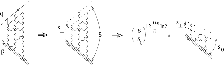
FIG. 1.: BFKL evolution in terms of Wilson-line operators (denoted by dotted lines).

The starting point of the evolution is the slope collinear to the momentum of the incoming photon q ($\zeta=x_{B}$) and it is convenient to stop the evolution at a certain intermediate point $\zeta_{0}={Q^{2}\over s_{0}}$ where $s_{0}\gg m_{N}^{2},~{}~{}{\alpha_{s}\over\pi}\ln{s_{0}\over m_{N}^{2}}\ll 1~{}$. The first of these conditions means that $s_{0}$ is still high from the viewpoint of low-energy nucleon physics while the second condition means that $s_{0}$ is sufficiently small from the viewpoint of high-energy physics (so one can neglect BFKL logs). The matrix element of the double-Wilson-line operator at this slope is a phenomenological input for the BFKL evolution (just as the structure function at low $Q^{2}$ serves as the input for ordinary DGLAP evolution). At large $s$ the integral over $\nu$ is dominated by the vicinity of $\nu=0$ which gives the familiar BFKL asymptotics:

$$\sigma^{\rm tot}\simeq x_{B}^{12{\alpha_{s}\over\pi}\ln 2}$$ (6)

Note, however, that the full nonlinear equation (4) contains more information than the linear BFKL equation — for example, it describes also the triple vertex of hard pomerons in QCD. In order to see that, it is convenient to consider some process which is dominated by the three-pomeron vertex — the best example is the diffractive dissociation of the virtual photon.

OPE for diffractive cross sections

The total cross section for diffractive scattering has the form:

$$\sigma^{\rm diff}_{\rm tot}=\int dxe^{iqx}\int{d^{3}p^{\prime}\over(2\pi)^{3}}\sum_{X}\langle p|j_{\mu}(x)|p^{\prime}+X\rangle\langle p^{\prime}+X|j_{\nu}(0)|p\rangle$$ (7)

where $\sum_{X}$ means the summation over all intermediate states. We can formally write down this cross section as a “diffractive matrix element”(cf ref. [4]):

$$\sigma^{\rm diff}_{\mu\nu}=\langle p|T\{j^{-}_{\mu}(x)j^{+}_{\nu}(0)e^{i\int dz({\cal L}^{+}(z)-{\cal L}^{-}(z))}\}|p\rangle_{\rm diff}$$ (8)

The index “$-$” marks the fields to the left of the cut and “$+$” to the right. The definition of the T-product of the fields with $\pm$ labels is as follows: the “$+$”fields are time-ordered, the “$-$”fields stand in inverse time order (since they correspond to the complex conjugate amplitude), and “$-$” fields stand always to the left of the “$+$”ones. Therefore, the diagram technique with the double set of fields is the following: contraction of two “$+$”fields is the usual Feynman propagator ${\not p\over p^{2}+i\epsilon}$ (for the quark field), contraction of two $``-^{\prime\prime}$ fields is the complex conjugated propagator ${\not p\over p^{2}-i\epsilon}$, and the contraction of the “$-$” field with the “$+$”one is the “cutted propagator” $2\pi\delta(p^{2})\theta(p_{0})\!\not\!p$ . This diagram technique for calculating T-products of double sets of fields exactly reproduces the Cutkosky rules for the calculation of cross sections.

The main result of this paper is the operator expansion for the diffractive amplitude $\sigma^{\rm diff}_{\mu\nu}$. Similarly to the case of the usual amplitude (1), we get in lowest order in $\alpha_{s}$:

$$\sigma^{\rm diff}_{\mu\nu}=\int d^{2}x_{\perp}I_{\mu\nu}(x_{\perp})\langle p|\mathop{\rm Tr}\{W(x)W^{\dagger}(0)\}|p\rangle_{\rm diff},$$ (9)

Here $W(x_{\perp})=V^{\dagger}(x_{\perp})U(x_{\perp})$ where $U(x_{\perp})$ denotes the Wilson-line operator (2) constructed from $``+^{\prime\prime}$ fields and $V(x_{\perp})$ from $``-^{\prime\prime}$ fields.

The evolution equation (with respect to the slope of the supporting line) turns out to have the same form as eq. (4) for usual amplitudes:

$$\zeta\frac{d}{d\zeta}{\cal W}(x_{\perp},y_{\perp})={3\alpha_{s}\over 2\pi^{2}}\int dz_{\perp}{(x_{\perp}-y_{\perp})^{2}\over(x_{\perp}-z_{\perp})^{2}(z_{\perp}-y_{\perp})^{2}}$$ (10)

$$\left\{{\cal W}(x_{\perp},z_{\perp})+{\cal W}(z_{\perp},y_{\perp})-{\cal W}(x_{\perp},y_{\perp})+{\cal W}(x_{\perp},z_{\perp}){\cal W}(z_{\perp},y_{\perp})\right\}$$ (11)

where ${\cal W}(x_{\perp},y_{\perp})\stackrel{{\scriptstyle\rm def}}{{\equiv}}{1\over 3}\mathop{\rm Tr}\{W(x_{\perp})W^{\dagger}(y_{\perp})\}-1$. Consequently, the linear evolution has the same form as (5).

Let us describe now the diffrractive amplitude in LLA and in leading order in $N_{c}$. In this approximation we must take into account the non-linearity in eq. (11) only once, and the rest of the evolution is linear. The result is (roughly speaking) the three two-gluon BFKL ladders which couple in a certain point — see Fig.2.

                                   

FIG. 2.: Amplitude of diffractive scattering in the LLA-$N_{c}$ approximation.

For the case of diffractive DIS, this evolution has the form (cf. ref. [5]):

$$\langle p|\int dy_{\perp}{\cal W}^{\zeta=x_{B}}(x_{\perp}+y_{\perp},y_{\perp})|p\rangle=$$ (12)

$$\displaystyle{3\alpha_{s}\over 8\pi^{3}}\int d\nu(x_{\perp}^{2})^{\frac{1}{2}+i\nu}\int d\nu_{1}d\nu_{2}dx_{1\perp}dx_{2\perp}\nu_{1}^{2}\nu_{2}^{2}\left((x_{1}-x_{2})_{\perp}^{2}\right)^{-\frac{1}{2}+i(\nu_{1}+\nu_{2}-\nu)}$$ (13)

$$\displaystyle\Theta(\nu;\nu_{1},\nu_{2})\int{d^{2}p^{\prime}_{\perp}\over 4\pi^{2}}\int^{s}_{Q^{2}}{dM^{2}\over M^{2}}\left({s\over M^{2}}\right)^{\omega(\nu)}\left({M^{2}\over Q^{2}}\right)^{\omega(\nu_{1})+\omega(\nu_{2})}$$ (14)

$$\langle p|{\cal U}^{\zeta_{0}}(x_{1\perp},\nu_{1}|p^{\prime}\rangle\langle p^{\prime}|{\cal U}^{\zeta_{0}}(x_{2\perp},\nu_{2})|p\rangle$$ (15)

where $M^{2}$ is the invariant mass of the produced particles,

$${\cal U}(x_{\perp},\nu)=\int dx_{\perp}^{\prime}dy_{\perp}^{\prime}\left({(x^{\prime}-y^{\prime})_{\perp}^{2}\over(x^{\prime}-x)_{\perp}^{2}(y^{\prime}-x)_{\perp}^{2}}\right)^{\frac{1}{2}+i\nu}{{\cal U}(x_{\perp}^{\prime},y_{\perp}^{\prime})\over(x^{\prime}-y^{\prime})_{\perp}^{4}}$$ (16)

is the eigenfunction[6] of the linear evolution equation (4) (at $t\not=0$) and $\Theta(\nu;\nu_{1},\nu_{2})$ is a certain numerical function of three $\nu$’s. (The coupling constant of three BFKL pomerons (6) is $\Theta(0;0,0)\simeq 1.58$). The value of $M^{2}$ determines the rapidity gap: from $\eta=\ln{s\over Q^{2}}$ to $\eta=\ln{M^{4}\over Q^{2}s}$ we have a production of particles described by the cut part of the ladder in Fig. 2 which brings in the factor $\left({s/M^{2}}\right)^{\omega(\nu)}$ while from $\eta=\ln{M^{4}\over Q^{2}s}$ to $\eta=\ln x_{B}$ we have a rapidity gap so there are two independent BFKL ladders which bring in the factors $\left({M^{2}/Q^{2}}\right)^{\omega(\nu_{1})}$ and $\left({M^{2}/Q^{2}}\right)^{\omega(\nu_{2})}$. The coupling of the BFKL pomeron with non-zero momentum transfer to the nucleon is decribed by the matrix element $\langle p^{\prime}|{\cal U}(x,\nu)|p\rangle$. At high energies and momentum transfer, it can be approximated by the non-forward gluon parton density.

REFERENCES

• [1] N. Cartiglia, ”Diffractive scattering at HERA”, hep-ph/9703245.
• [2] I. Balitsky, Nucl. Phys. B463, 99 (1996).
• [3] V.S. Fadin, E.A. Kuraev, and L.N. Lipatov, Phys. Lett.60B,50 (1975)
I. Balitsky and L.N. Lipatov,Sov. J. Nucl. Phys.28,822 (1978)
• [4] I. Balitsky and V.M. Braun, Phys. Lett.B222,123 (1989); Nucl. Phys. B361, 93 (1991).
• [5] I. Bartels and M. Wuesthoff, Z. Phys. C66, 157 (1995).
• [6] L.N. Lipatov Sov. Phys. JETP 63, 904 (1986)