Abstract

We compare vector boson fusion and quark antiquark annihilation production of vector boson pairs at the LHC and include the effects of anomalous couplings. Results are given for confidence intervals for anomalous couplings at the LHC assuming that measurements will be in agreement with the standard model. We consider all couplings of the general triple vector boson vertex and their correlations. In addition we consider a gauge invariant dimension-six extension of the standard model. Analytical results for the cross sections for quark antiquark annihilation and vector boson fusion with anomalous couplings are given.

1 Introduction

In this note we study vector boson pair production with possible anomalous couplings in proton proton collisions at the LHC. The motivation to study these processes has been twofold:

1. If the electroweak symmetry breaking is not realized by a light Higgs boson, the symmetry breaking will manifest itself by some strong interactions among longitudinally polarized gauge bosons [1, 2]. In general, the amplitudes for longitudinal vector boson scattering are then very large at high energies. Several models to describe the strongly coupled symmetry breaking, in particular the standard model with a heavy Higgs boson and technicolor inspired models, have been discussed [3, 4, 5, 6]. If an amplitude has been calculated within a specific model, a method to connect this amplitude to parton parton scattering processes has to be employed. The conventional method [7, 8, 9, 10] was to use the effective vector boson approximation (EVBA) [11]. The EVBA was originally used only for longitudinally polarized vector bosons. It was however also applied to all intermediate helicity states [5] despite of the known problems with the EVBA for the transverse helicities [12].

   Avoiding the use of the EVBA, the quark-quark scattering processes $q_{1}q_{2}\to V_{3}V_{4}q_{1}^{\prime}q_{2}^{\prime}$ were calculated exactly in lowest order of perturbation theory [3, 6]. In addition to the vector boson scattering diagrams, diagrams of bremsstrahlung type have to be evaluated in the exact calculation.

2. On the other hand one may assume that the symmetry breaking is realized by a light Higgs boson. In this case the dominating processes for vector boson pair production are those of direct quark antiquark annihilation, also called Drell-Yan processes. The rates for these processes are sensitive to the values of the couplings of the electroweak vector bosons among each other [13]. Drell-Yan production with anomalous (=non-standard) couplings has been studied in [14]-[20]. ${O}(\alpha_{s})$ corrections have been taken into account in [21]-[26]. The vector boson scattering processes were not considered in these works. The common argument to omit these processes was that they are ${O}(\alpha^{4})$ and therefore suppressed with respect to the Drell-Yan processes. However, a particular case in which these processes can give a significant contribution is near a Higgs boson resonance. In the study [27] of the signal of a resonant Higgs boson both the Drell-Yan processes, including the ${O}(\alpha_{s})$ corrections [28], and the exact matrix element for $q_{1}q_{2}\to V_{3}V_{4}q_{1}^{\prime}q_{2}^{\prime}$ were taken into account. Also in [29], the processes $q_{1}q_{2}\to V_{3}V_{4}q_{1}^{\prime}q_{2}^{\prime}$ were included. These calculations however were only for standard vector boson self couplings and the rates for the two different production mechanisms have not been explicitly compared.

In summary, in the strongly interacting scenario particular attention was paid to the vector boson scattering processes while the analyses of vector boson self couplings only considered the Drell-Yan processes.

Later on, the effects of various $SU(2)_{L}\times U(1)_{Y}$ gauge invariant effective interaction terms among the electroweak vector bosons were investigated and the vector boson scattering processes were considered [30, 31] together with the Drell-Yan processes. It was found that the Drell-Yan contribution and the one of vector boson scattering were of comparable magnitude. However, as in [5], the vector boson scattering processes were calculated using the EVBA for all intermediate boson helicities.

Recently [32, 33] we showed that an improved version of the EVBA can increase the reliability of EVBA calculations. In particular, the improved EVBA could well reproduce the result of a complete perturbative calculation for a process which is dominated by the transverse intermediate helicities.

In this article we carry out a comparison of Drell-Yan production and vector boson scattering using the improved EVBA and including the influence of anomalous couplings. This work is thus a supplement to the existing analyses [14, 24, 25, 26] in which the Drell-Yan processes have been considered in more detail ($O(\alpha_{s})$ corrections were included and more refined kinematical cuts were applied), but vector boson scattering was not discussed. We will study the general parametrization [16],[34]-[38] of the triple gauge boson vertices in terms of seven parameters, allowing for $C$- and $P$-violation. In addition, we will study an $SU(2)_{L}\times U(1)_{Y}$ gauge invariant dimension-six extension of the standard model. Our work extends the works [30, 31] in that all three $C$- and $P$-invariant gauge invariant dimension-six operators [39]-[42] which affect the vector boson self-interactions are discussed. We note that the three $C$- and $P$-invariant trilinear couplings which potentially contribute to the experimentally relevant [13] process of $W^{\pm}Z$ Drell-Yan production can be equivalently expressed in terms of the parameters of the three-parameter gauge invariant model. The same is true for the two $C$- and $P$-invariant couplings which potentially contribute to the similarly relevant process of $W^{\pm}\gamma$ production.

In Section 2 we compare vector boson fusion and Drell Yan production in the three-parameter gauge invariant model. In Section 3, we present parameter fits for the anomalous couplings which can be obtained from future LHC measurements assuming that standard model predictions will actually be measured. We discuss the full set of anomalous couplings and also give the unitarity limits for the set of couplings which we use. We also consider again the three-parameter gauge invariant model. In Appendix A we give analytical formulas for the cross sections for $q\bar{q}^{\prime}$ annihilation into $W^{\pm}Z,W^{\pm}\gamma$ and $W^{+}W^{-}$ pairs in terms of the seven anomalous couplings. In Appendix B we give formulas for vector boson scattering cross sections for the gauge invariant model.

2 Comparison of Vector-Boson Fusion and Drell-Yan Production

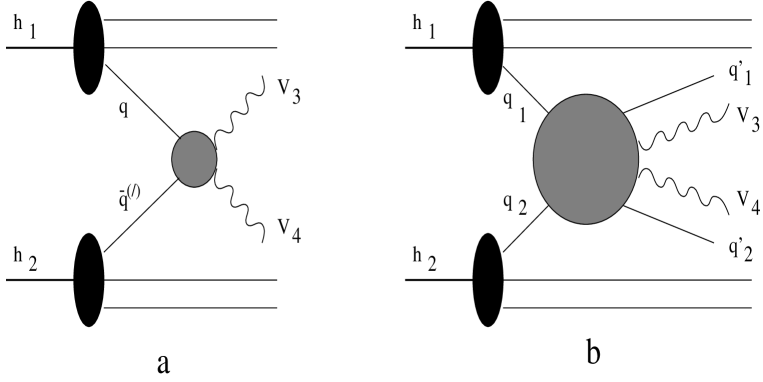
Figure 1: Diagrammatic representations for the production of a vector boson pair $V_{3}V_{4}$ in the collision of two hadrons $h_{1}h_{2}$. a: via the quark antiquark annihilation mechanism. b: via the ${O}(\alpha^{4})$ parton reaction $q_{1}q_{2}\to V_{3}V_{4}q^{\prime}_{1}q^{\prime}_{2}$.

To illustrate our results we calculate the invariant mass distributions of the cross sections for vector boson pair production at the LHC ($pp$ collisions at $\sqrt{s_{pp}}=14$ TeV). We compute both the contribution from Drell-Yan production and from the ${O}(\alpha^{4})$ parton reaction $q_{1}q_{2}\to V_{3}V_{4}q_{1}^{\prime}q_{2}^{\prime}$ which contains vector boson scattering. The two contributions are shown diagrammatically in Figure 1. Both contributions are calculated in the Born approximation and we use the improved EVBA [32, 33] to calculate the latter contribution. We discuss all possible pairs of produced electroweak vector-bosons, $W^{\pm}Z,W^{\pm}\gamma,W^{+}W^{-},ZZ,W^{\pm}W^{\pm},Z\gamma$ and $\gamma\gamma$. We first present the results for the standard model and then for non-zero anomalous couplings.

2.1 Calculational Procedure

2.1.1 Drell-Yan Production

In the usual quark-parton description, the lowest order contribution comes from the Drell-Yan processes shown in Figure 1 (a). Three generic Feynman diagrams can contribute to any of these processes in lowest order (Fig. 2). They correspond to the exchange of vector boson(s) in the $s$-channel and the exchange of fermions in the $t$- and in the $u$-channel. Only the vector-boson exchange diagrams receive a contribution from the vector boson self-couplings. The standard model differential cross sections for $q\bar{q}^{\prime}\to V_{3}V_{4}$ have been first given in [43]. The results for arbitrary $\alpha_{W}$ can be found in [30]. For arbitrary vector boson self couplings, demanding only Lorentz-invariance, the differential cross sections as well as the expressions for the helicity amplitudes have been recently given for all processes in analytical form in [44]. We choose to repeat the formulas for the differential cross sections in Appendix A in a form in which the high energy behavior is immediately transparent. We note that the ${O}(\alpha_{s})$-corrections to the lowest order cross-sections can be huge. For $W^{\pm}Z$ production [25] they can reach up to 70% of the lowest order contribution and for $W^{\pm}\gamma$ production [20] they can be even larger. Only the Born cross section will be considered here.

The formula for the invariant mass distribution of the cross section for $V_{3}V_{4}$-pair production via $q\bar{q}^{\prime}$-annihilation in the collision of two hadrons $h_{1}h_{2}$ is given by

$$\frac{d\sigma}{dM_{V_{3}V_{4}}}(h_{1}h_{2}\to q\bar{q}^{\prime}\to V_{3}V_{4},s_{hh})|_{\mathrm{cut}}$$ (1)

$$= \frac{2M_{V_{3}V_{4}}}{s_{hh}}\int\limits_{-y_{\mathrm{max}}}^{y_{\mathrm{max}}}dy\sum_{(q\bar{q}^{\prime})}\left[f_{q}^{h_{1}}(\sqrt{x}e^{y},Q_{1}^{2})f_{\bar{q}^{\prime}}^{h_{2}}(\sqrt{x}e^{-y},Q_{2}^{2})\;\;+\;\;h_{1}\leftrightarrow h_{2}\;\right]$$ (3)

$$\quad\quad\quad\times\int\limits_{z_{\mathrm{min}}(y)}^{z_{\mathrm{max}}(y)}d\cos\theta\frac{d\sigma}{d\cos\theta}(q\bar{q}^{\prime}\to V_{3}V_{4}).$$

This formula is valid if either no cuts or a rapidity or a pseudorapidity cut on both produced vector bosons is applied. A pseudorapidity cut, in contrast to a rapidity cut, always excludes events near the hadron beam direction. In (3), $\sqrt{s_{hh}}$ and $M_{V_{3}V_{4}}$ are the invariant masses of the hadron pair and the vector boson pair, respectively, $y$ is the rapidity of the $q\bar{q}^{\prime}$-pair in the $h_{1}h_{2}$ c.m.s and $x\equiv M_{V_{3}V_{4}}^{2}/s_{hh}$. The quantities $f_{q}^{h_{i}}$ denote the parton distributions in the hadrons and the quantities $Q_{i}^{2}$ are the factorization scales. $\theta$ is the angle between the quark $q$ and the vector-boson $V_{3}$ in the center-of-mass system of the quarks. Applying no cuts, the limits of integration in (3) are $y_{\mathrm{max}}=\frac{1}{2}\ln(1/x)$ and $z_{\mathrm{min}}(y)=z_{\mathrm{max}}(y)=1$. We choose here to apply a pseudorapidity cut $\eta$ on the produced vector bosons. This cut is equivalent to a minimum required angle $\vartheta_{\mathrm{min}}$ between the direction of momentum of any of the produced vector-bosons and the hadron beam direction. The cut $\eta$ is related to $\vartheta_{\mathrm{min}}$ by $\tanh(\eta)\equiv\cos\vartheta_{\mathrm{min}}$. The integration limits with an $\eta$-cut in the $h_{1}h_{2}$ c.m.s are given by

$$y_{\mathrm{max}} = \min\left[\frac{1}{2}\ln\left(\frac{1}{x}\right),\tanh^{-1}\left(\sqrt{\frac{1}{1+(\min(E_{3}^{2},E_{4}^{2})/q^{2})\tan^{2}\vartheta_{\mathrm{min}}}}\right),\right.$$ (5)

$$\left.\quad\quad\quad\quad\quad\quad\quad\!\tanh^{-1}\left(\sqrt{\frac{1}{1+(\max(M_{3}^{2},M_{4}^{2})/q^{2})\sin^{2}\vartheta_{\mathrm{min}}}}\right)\right],$$

$$z_{\mathrm{min}\atop\mathrm{max}}(y) = \frac{1}{q(1+t^{2}\gamma^{2})}{\max\atop\min}\left[-t^{2}\gamma^{2}\beta E_{3}\mp\sqrt{q^{2}(1+t^{2}\gamma^{2})-t^{2}\gamma^{2}\beta^{2}E_{3}^{2}}\right.,$$ (7)

$$\quad\quad\quad\quad\quad\quad\quad\quad\;\,\left.t^{2}\gamma^{2}\beta E_{4}\mp\sqrt{q^{2}(1+t^{2}\gamma^{2})-t^{2}\gamma^{2}\beta^{2}E_{4}^{2}}\right],$$

and one has to require that $z_{\mathrm{min}}<z_{\mathrm{max}}$. The upper sign of $\mp$ in (7) is for $z_{\mathrm{min}}$, the lower sign for $z_{\mathrm{max}}$. In (7), the quantity $\beta\equiv\tanh(y)$ is the boost-parameter for a transformation from the $(h_{1}h_{2})$ c.m.s into the $(V_{3}V_{4})$ (=$(q\bar{q}^{\prime})$) c.m.s. and $t^{2}\equiv\tan^{2}\vartheta_{\mathrm{min}}$. Further we defined $\gamma^{2}\equiv 1/(1-\beta^{2})$. The quantities $E_{3}\equiv\sqrt{q^{2}+M_{3}^{2}}$ and $E_{4}\equiv\sqrt{q^{2}+M_{4}^{2}}$ are the energies of $V_{3}$ and $V_{4}$ in the $(q\bar{q}^{\prime})$ cms, while $M_{3}$ and $M_{4}$ are their masses. $q$ is the magnitude of the three-momentum of $V_{3}$ or $V_{4}$ in the $(V_{3}V_{4})$ cms-system. The last argument of the $\min$-function which defines $y_{\mathrm{max}}$ in (7) only plays a role near the threshold. In deriving (7) we assumed that the quarks have no transverse momentum with respect to the hadrons, but no other kinematical approximations were made.

For large energies of the produced vector-bosons, $q^{2}\gg\max(M_{3}^{2},M_{4}^{2})$, the limits of integration (7) take on the simplified forms

$$y_{\mathrm{max}} \simeq \min\left[\frac{1}{2}\ln\left(1/x\right),\eta\right],$$ (8)

$$z_{\mathrm{max}}(y) \simeq -z_{\mathrm{min}}(y)\;\simeq\;\tanh(\eta-|y|).$$ (9)

In this limit, the $\eta$-cut is identical to a rapidity-cut $Y$ of the same magnitude. We choose a cut of the magnitude $\eta=1.5$, corresponding to a minimum angle of $\theta_{\mathrm{min}}=25^{0}$. For the relevant process $pp\to W^{\pm}Z+X$ the highest sensitivity to anomalous couplings is achieved with a cut of about this magnitude [45].

Figure 2: The generic Feynman diagrams for a process $q\bar{q}^{\prime}\to V_{3}V_{4}$ in lowest order of perturbation theory.

2.1.2 Vector Boson Fusion

The ${O}(\alpha^{4})$ partonic reaction which is shown in Figure 1 (b) contains the vector-boson scattering processes $V_{1}V_{2}\to V_{3}V_{4}$ as subprocesses. Three types of Feynman diagrams contribute to a generic process $V_{1}V_{2}\to V_{3}V_{4}$. They correspond to vector boson exchange, a direct interaction among the four vector bosons and Higgs boson exchange. Using the Feynman rules for the GIDS model given in [46] we wrote the amplitudes as functions of the scalar products of the external momenta and of polarization vectors. We evaluated them numerically without making further approximations. In Appendix B we give analytical expressions for the cross sections for $W^{\pm}Z\to W^{\pm}Z$, $W^{\pm}\gamma\to W^{\pm}Z$ and $W^{\pm}\gamma\to W^{\pm}\gamma$ in a high energy approximation. Expressions for the amplitudes of these and other vector boson scattering processes can be found in [31, 46, 47].

We calculate the invariant mass distribution of the cross-section for $h_{1}h_{2}\to V_{1}V_{2}\to V_{3}V_{4}$ in the improved EVBA according to [33]. The formulas which have been given there apply if a rapidity cut is used. The corresponding expressions for a pseudorapidity cut are obtained by replacing $z_{\mathrm{min}}(y),z_{\mathrm{max}}(y)$ and $y_{\mathrm{max}}$ in [33] by the expressions (7). We use the exact vector boson pair luminosities of [33] if $V_{1}V_{2}$ consists of two massive vector bosons. If a photon is involved, the Approximation 2 of [33] with the photon distribution function of [48] is used.

2.2 Results in the Standard Model

Figs. 3,4 and 5 show the invariant mass distributions for all vector boson pair production processes in the standard model. We separately show the contributions from the processes $V_{1}V_{2}\to V_{3}V_{4}$ and those from $q\bar{q}^{\prime}\to V_{3}V_{4}$. The mass of the Higgs boson was chosen to be $M_{H}=300$ GeV. There is little effect (less than 15% of change in the contribution from vector boson fusion) on the results for $W^{\pm}Z$ and $W^{\pm}\gamma$ production if the mass of the Higgs boson is varied in between $M_{H}=0.1$ TeV and $M_{H}=0.8$ TeV. The other electroweak parameters were chosen as $\alpha=1/128,M_{Z}=91.19$ GeV and $M_{W}=80.33$ GeV. We use the Higgs boson width $\Gamma_{H}$ for the dominant decay modes into $W^{+}W^{-}$ and $ZZ$, $\Gamma_{H}=\Gamma_{H\to W^{+}W^{-}}+\Gamma_{H\to ZZ}$, where

$$\Gamma_{H\to VV}=\frac{\alpha M_{H}^{3}}{n!64s_{W}^{2}M_{W}^{2}}\sqrt{1-x_{V}}(4-4x_{V}+3x_{V}^{2}).$$ (10)

In (10), $x_{V}\equiv 4M_{V}^{2}/M_{H}^{2}$ and $s_{W}^{2}\equiv\sin^{2}(\theta_{W})$, where $\theta_{W}$ is the weak mixing angle. $n$ is the number of identical particles in the state $VV$. For the parton distribution functions we use the set MRS(R2) [49] which includes the latest HERA data and uses $\alpha_{s}(M_{Z}^{2})=0.120$ as input parameter, a value favored by the LEP 1 data. A contribution from top quarks is neglected. For the scales $Q_{i}^{2}$ appearing as arguments of the parton distribution functions we use the quark-quark sub-energy, $Q_{i}^{2}=s_{qq}$. For the elements of the CKM matrix we take $|V_{ud}|^{2}=|V_{cs}|^{2}=0.95$, $|V_{us}|^{2}=|V_{cd}|^{2}=0.05$ and consequently assume no mixing of the third flavor with the other two flavors. If no CKM mixing is included at all none of the differential cross sections changes by more than 1%.

Figs. 3 to 5 clearly show that the contribution from vector boson scattering is always an order of magnitude smaller than the contribution from $q\bar{q}^{\prime}$-annihilation (also if the sum over all $V_{1}V_{2}$ is taken). The contribution may therefore indeed be neglected.

Fig. 6 shows the ratio of the cross sections for $pp\to W^{\pm}(\gamma,Z)\to W^{\pm}Z$ ($W^{\pm}Z$ production $\equiv$ the sum of $W^{+}Z$ and $W^{-}Z$ production, $W^{\pm}(\gamma,Z)$ intermediate states $\equiv$ the sum of $W^{\pm}\gamma$ and $W^{\pm}Z$ intermediate states) and for $pp\to q\bar{q}^{\prime}\to W^{\pm}Z$ as a function of $M_{V_{3}V_{4}}$. The ratio of the integrated cross sections is 12% (15%) for a cut of $\eta=1.5$ ($\eta=2.5$).

Figure 3: The cross sections for $W^{+}Z,W^{-}Z,W^{+}\gamma$ and $W^{-}\gamma$ production as functions of the invariant mass $M_{V_{3}V_{4}}$ of the produced vector boson pair for $pp$-collisions at $\sqrt{s}=14$ TeV. Separately shown are the contributions from $q\bar{q}^{\prime}$-annihilation and from vector-boson fusion processes. A rapidity cut of $\eta=1.5$ has been applied.

Figure 4: The cross sections for $W^{+}W^{-},ZZ,W^{+}W^{+}$ and $W^{-}W^{-}$ production as functions of the invariant mass $M_{V_{3}V_{4}}$ of the produced vector boson pair for $pp$-collisions at $\sqrt{s}=14$ TeV. Separately shown are the contributions from $q\bar{q}^{\prime}$-annihilation and from vector-boson fusion processes. A pseudorapidity cut of $\eta=1.5$ has been applied.

Figure 5: The same as Fig. 4 but for $Z\gamma$ and $\gamma\gamma$ production.

Figure 6: The ratio of the cross sections for $pp\to W^{\pm}(Z,\gamma)\to W^{\pm}Z$ and $pp\to q\bar{q}^{\prime}\to W^{\pm}Z$ as a function of the invariant mass $M_{V_{3}V_{4}}$ for $\sqrt{s_{pp}}=14$ TeV.

We note that a different value of this ratio is obtained if the EVBA in leading logarithmic approximation (LLA) is used instead. In [4, 5] the cross sections for $pp\to W^{\pm}(\gamma,Z)\to W^{\pm}Z$ and for $pp\to q\bar{q}^{\prime}\to W^{\pm}Z$ were calculated and the LLA EVBA was used. Calculating the ratio of these cross sections, we obtain 57% for $Y=1.5$ and 64% for $Y=2.5$ for the case of a light Higgs boson (59% ($Y=1.5$) and 65% ($Y=2.5$) for $M_{H}=1$ TeV). Likewise, if we repeat the calculation of [30, 31] (we used $\eta=1.5$, $M_{H}=0.1$ TeV and integrated the cross sections in the region 0.5 TeV $<M_{WZ}<$ 2 TeV), we obtain a value of 52% for the ratio. For more details we refer to [45].

These values of the ratio are thus much higher than the values obtained with the improved EVBA. The latter values are however in agreement with values following from [6], in which a complete (lowest order) calculation of the processes $q_{1}q_{2}\to q^{\prime}_{1}q^{\prime}_{2}W^{+}Z$ was carried out instead of an EVBA. Computing the ratio of the cross sections for $pp\to q_{1}q_{2}\to q_{1}^{\prime}q_{2}^{\prime}W^{+}Z$ and $pp\to q\bar{q}^{\prime}\to W^{+}Z$ given in [6] one obtains 17% (21%) for $M_{H}=0.1$ TeV ($M_{H}=1$ TeV). In summary, the improved EVBA calculation and the complete calculation both yield a value for the ratio which is between 10% and about 20%, while calculations using the LLA EVBA yield a value which is larger by more than a factor of 3.

We remark that for $M_{H}=300$ GeV even the Higgs boson peak (which is present only in $W^{+}W^{-}$ and $ZZ$ production) stays below the rate of $q\bar{q}^{\prime}$-annihilation. We finally note that the like-charge pair production processes $pp\to W^{\pm}W^{\pm}+X$ cannot proceed via $q\bar{q}^{\prime}$ annihilation and might thus allow to directly observe vector boson scattering.

2.3 Parametrization of Anomalous Couplings

The model we use for the anomalous couplings was described in [42] (GIDS model). In this model, the most general $SU(2)_{L}\times U(1)_{Y}$-symmetric interaction terms of dimension six are added to the Lagrangian of the standard model. We restrict ourselves to $C$- and $P$-conserving interactions which contain no higher derivatives and explicitly contain vector boson self-interactions. There are three of those interaction terms which are described by the parameters $\alpha_{W},\alpha_{W\Phi}$ and $\alpha_{B\Phi}$. They are related to the usual parameters [37] $x_{\gamma},y_{\gamma}$ and $\delta_{Z},x_{Z},y_{Z}$, which parametrize the $C$- and $P$-conserving interactions of the $\gamma W^{+}W^{-}$ and the $ZW^{+}W^{-}$ vertex, respectively, by

$$\delta_{Z}=\frac{c_{W}}{s_{W}}\Delta g_{1}^{Z}=\frac{\alpha_{W\Phi}}{s_{W}c_{W}},\;\,x_{Z}=\frac{c_{W}}{s_{W}}(\Delta\kappa_{Z}-\Delta g_{1}^{Z})=-\frac{s_{W}}{c_{W}}(\alpha_{W\Phi}+\alpha_{B\Phi})=-\frac{s_{W}}{c_{W}}x_{\gamma},$$

$$y_{Z}=\frac{c_{W}}{s_{W}}\lambda_{Z}=\frac{c_{W}}{s_{W}}\alpha_{W},\quad x_{\gamma}=\Delta\kappa_{\gamma}=\alpha_{W\Phi}+\alpha_{B\Phi},\quad y_{\gamma}=\lambda_{\gamma}=\alpha_{W}.$$ (11)

In (11) we also included the relations to the parameters $\Delta g_{1}^{Z},\Delta\kappa_{Z},\lambda_{Z}$ and $\Delta\kappa_{\gamma},\lambda_{\gamma}$ of [17].

The reduction from the five parameter case of $\delta_{Z},x_{Z},y_{Z},x_{\gamma}$ and $y_{\gamma}$ to the three parameter case is manifest through the relations $x_{Z}=-(s_{W}/c_{W})x_{\gamma}$ and $y_{Z}=(c_{W}/s_{W})y_{\gamma}$ which are implicit in (11). The three parameter model defined in (11) has already been obtained [42] in [16, 35] from the assumption of a custodial $SU(2)$ symmetry. The relation between $x_{\gamma}$ and $x_{Z}$ in (11), $x_{Z}=-(s_{W}/c_{W})x_{\gamma}$, is a consequence of the exclusion of intrinsic $SU(2)$ violation, i.e., of $SU(2)$ custodial symmetry. The relation between $y_{\gamma}$ and $y_{Z}$ in (11) follows from the requirement of $SU(2)_{L}\times U(1)_{Y}$ symmetry in the quadrupole interactions. In addition to trilinear interactions the three-parameter dimension-six $SU(2)_{L}\times U(1)_{Y}$ gauge invariant model describes interactions among four and more vector bosons. Also these interactions are already contained in an identical form [42] in the model described in [16, 35]. The only difference [50] of the three-parameter model [16, 35] and the $SU(2)_{L}\times U(1)_{Y}$ invariant one lies in non-standard interactions of the Higgs boson.

We note that there are no non-standard interactions among three neutral gauge bosons which would obey $C$- and $P$-symmetry, contain no higher derivatives and are compatible with electromagnetic gauge and Lorentz invariance [36].

The Lagrangian of the GIDS model is an effective, unrenormalizable one and can in general be written as [51]

$${\cal L}_{\mathrm{eff}}={\cal L}_{0}+\sum_{j}\frac{\tilde{g_{j}}}{\Lambda}{\cal L}_{j}^{(5)}+\sum_{j}\frac{\tilde{g_{j}}}{\Lambda^{2}}{\cal L}_{j}^{(6)}+\ldots\;.$$ (12)

In (12), ${\cal L}_{0}$ is the Lagrangian of the standard model, the ${\cal L}_{j}^{(d)}$ are interaction terms of dimension $d$, the $\tilde{g_{j}}$ are coupling constants and $\Lambda$ is the energy scale of new physics. We assumed the same (gauge) symmetries for the ${\cal L}_{j}^{(d)}$ as for ${\cal L}_{0}$. This implies that the ${\cal L}_{j}^{(5)}$ term (and all terms with an odd $d$) in (12) are absent. If we further assume that the $\tilde{g}_{j}$ are of the same order of magnitude as the standard model couplings $g$,$g^{\prime}$ and $e$ and compare the Lagrangian (12) with the one defining the $\alpha$-parameters [42], we read off the order of magnitude for the $\alpha$-parameters,

$$\alpha_{W},\alpha_{W\Phi},\alpha_{B\Phi}=O\left(M_{W}^{2}/\Lambda^{2}\right).$$ (13)

Assuming $\Lambda\;\raisebox{-3.00003pt}{$\stackrel{{\scriptstyle\displaystyle>}}{{\sim}}$}\;2$ TeV (and consequently restricting ourselves to scattering energies up to $M_{V_{3}V_{4}}<2$ TeV), the order of magnitude for the $\alpha$-parameters is

$$\alpha_{W},\alpha_{W\Phi},\alpha_{B\Phi}\;\raisebox{-3.00003pt}{$\stackrel{{\scriptstyle\displaystyle<}}{{\sim}}$}\;{O}\left(10^{-3}\right).$$ (14)

The restrictions derived from partial wave unitarity applied to vector boson scattering amplitudes are [47]:

$$\left|\frac{s\alpha_{W}}{M_{W}^{2}}\right|\;\raisebox{-3.00003pt}{$\stackrel{{\scriptstyle\displaystyle<}}{{\sim}}$}\;\sqrt{\frac{12s_{W}^{2}}{\alpha}}\simeq 19,\quad\left|\frac{s\alpha_{W\Phi}}{M_{W}^{2}}\right|\;\raisebox{-3.00003pt}{$\stackrel{{\scriptstyle\displaystyle<}}{{\sim}}$}\;15.5,\quad\left|\frac{s\alpha_{B\Phi}}{M_{W}^{2}}\right|\;\raisebox{-3.00003pt}{$\stackrel{{\scriptstyle\displaystyle<}}{{\sim}}$}\;49,$$ (15)

where we have introduced $s\equiv M_{V_{3}V_{4}}^{2}$. For $\sqrt{s}\leq 2$ TeV the unitarity bounds (15) are

$$|\alpha_{W}|\leq 0.031,\quad\quad|\alpha_{W\Phi}|\leq 0.025,\quad\quad|\alpha_{B\Phi}|\leq 0.079.$$ (16)

These limits are larger than the values in Eq. (14) for the $\alpha^{\prime}s$ which we expect from the effective Lagrangian ansatz. Therefore, if the couplings are not larger than expected from the effective Lagrangian ansatz, unitarity is not violated for energies $\sqrt{s}\leq 2$ TeV. In [17, 20, 25, 26] a form factor assumption is made in order to avoid violation of unitarity. In our fits we follow the simple prescription to vary the coupling parameters within their unitarity limits only. In fact it will turn out that within the 95% CL limits the unitarity limits are never reached. Thus, in order to derive sensible experimental bounds on the anomalous couplings, one does not have to use form factors for which additional (unknown) parameters must be introduced.

If one nevertheless introduces a form factor, the couplings $\alpha_{i}$ which are to be inserted in the expressions for the cross sections are energy dependent. They are related to bare (energy independent) coupling constants, $\alpha_{i}^{0}$, by

$$\alpha_{i}=\frac{\alpha_{i}^{0}}{\left(1+\frac{\textstyle s}{\textstyle\Lambda_{FF}^{2}}\right)^{\textstyle n}}.$$ (17)

The bare coupling constants are those which appear in the Lagrangian. A usual choice for the exponent $n$ in (17) is $n=2$. Similar to $\Lambda$ in (12) $\Lambda_{FF}$ is an energy scale for new physics. The unitarity limits for the parameters $\alpha_{i}^{0}$ are obtained by inserting (17) into (15). We use $n=2$ and minimize the maximum value for $|\alpha_{i}^{0}|$ with respect to $s$. The minimum occurs at $s=\Lambda_{FF}^{2}$ and the unitarity limits are given by

$$|\alpha_{W}^{0}|\;\raisebox{-3.00003pt}{$\stackrel{{\scriptstyle\displaystyle<}}{{\sim}}$}\;76(M_{W}^{2}/\Lambda_{FF}^{2})\simeq 0.123,\quad\quad|\alpha_{W\Phi}^{0}|\;\raisebox{-3.00003pt}{$\stackrel{{\scriptstyle\displaystyle<}}{{\sim}}$}\;62(M_{W}^{2}/\Lambda_{FF}^{2})\simeq 0.100,$$

$$|\alpha_{B\Phi}^{0}|\;\raisebox{-3.00003pt}{$\stackrel{{\scriptstyle\displaystyle<}}{{\sim}}$}\;196(M_{W}^{2}/\Lambda_{FF}^{2})\simeq 0.316.$$ (18)

The numerical values in (18) are for $\Lambda_{FF}=2$ TeV. At multi-TeV colliders the cross section for fixed $\alpha_{i}^{0}\neq 0$ is very different from the cross section for fixed $\alpha_{i}$ and the obtainable bounds on the $\alpha_{i}$ are very much tighter than those for the $\alpha_{i}^{0}$. The distinction between the two models does however not very much affect the analysis of present Tevatron data since there the form factor is close to the value 1 as $\sqrt{s}$ can hardly be greater than 0.5 TeV.

2.4 Results with Anomalous Couplings

Fig. 7 shows the comparison of $q\bar{q}^{\prime}$-annihilation and vector boson fusion in the presence of anomalous couplings. We show the results for the relevant processes of $W^{\pm}Z$ and $W^{\pm}\gamma$ production and for $W^{+}W^{-}$ production. In addition, we present a plot for $W^{\pm}W^{\pm}$ production. We sum over the charge conjugated final states i.e. discuss the cross sections for $W^{\pm}V\equiv W^{+}V+W^{-}V$ and $W^{\pm}W^{\pm}\equiv W^{+}W^{+}+W^{-}W^{-}$ production. We have also summed over all $V_{1}V_{2}$ pairs. We only vary one coupling at a time. Only those couplings which lead to enhanced terms at high energies (i.e. of ${O}(\alpha_{i}s)$ or ${O}(\alpha_{i}^{2}s^{2})$) in the $q\bar{q}^{\prime}$ cross section are varied. Varying the other couplings leaves the $q\bar{q}^{\prime}$ cross sections virtually unchanged. For $W^{\pm}W^{\pm}$ production we vary all couplings. We choose a single non-zero magnitude for each of the couplings which is already quite large for the effective Lagrangian expectation, (14), but which is still below the unitarity limit (15). For $\alpha_{W}$ and $\alpha_{W\Phi}$ we take $|\alpha_{i}|=0.01$. For $\alpha_{B\Phi}$ we take $|\alpha_{B\Phi}|=0.03$. For the relevant processes of $W^{\pm}V$ production, we choose a negative and a positive value for the coupling if there is an enhanced term linear in the coupling.

The main conclusion from Fig. 7 is that vector boson scattering is only marginally important even if the anomalous couplings are different from zero. When constraining anomalous couplings using these processes, vector boson scattering might therefore well be omitted. The non-enhanced terms ($\alpha_{B\Phi}$ in $W^{\pm}Z$-production, $\alpha_{W\Phi}$ and $\alpha_{B\Phi}$ in $W^{\pm}\gamma$-production) are unlikely to lead to any observable effect at the LHC. Fig. 7 (d) shows that the effect of anomalous couplings for like-charge $W^{\pm}$-pair production is not very large.

Figure 7: The cross-sections for $W^{\pm}Z(\equiv W^{+}Z+W^{-}Z),W^{\pm}\gamma,W^{+}W^{-}$ and $W^{\pm}W^{\pm}(\equiv W^{+}W^{+}+W^{-}W^{-})$ production as functions of the invariant mass $M_{V_{3}V_{4}}$ of the produced vector boson pair for $pp$-collisions at $\sqrt{s}=14$ TeV. Various values of the anomalous couplings have been chosen. Separately shown are the contribution from $q\bar{q}^{\prime}$-annihilation and the (summed) contribution from vector boson fusion processes. A pseudorapidity cut of $\eta=1.5$ has been applied.

3 Parameter Fits for Anomalous Couplings

In this section we present parameter fits to fictitious standard model data and derive limits for the anomalous couplings. Refering to the conclusion of Section 2, we will take into account only the contribution from $q\bar{q}^{\prime}$ annihilation. First we consider $W^{\pm}\gamma$ and $W^{\pm}Z$ production separately. These are the experimentally relevant production processes [13]. The detection of a $W^{+}W^{-}$ pair is experimentally plagued by a large background of $t\bar{t}$ production with the subsequent decay of a top quark into a $W^{\pm}$ boson and a $b$ quark [13]. We use the general parametrization of the triple gauge boson vertices [36, 37, 38] in terms of seven free parameters, thus allowing for $C$- and $P$-violation. Then we present a fit to combined $W^{\pm}\gamma$ and $W^{\pm}Z$ “data” for the three parameter gauge invariant model. We take into account the full correlations among the parameters. Before we proceed we present the unitarity limits for the set of couplings which we are using [38, 44]. As far as we know, these limits have never been given before.

3.1 Unitarity Limits for $\delta_{V},x_{V},y_{V},z_{V},z^{\prime}_{1V},z^{\prime}_{2V}$ and $z^{\prime}_{3V}$

Theoretical bounds on anomalous couplings can be obtained by applying partial wave unitarity to the amplitudes for $q\bar{q}^{\prime}\to V_{3}V_{4}$. Inequalities derived from the requirement of partial wave unitarity have been given in [52]. The inequalities have been written in terms of “reduced amplitudes” for $q\bar{q}^{\prime}\to W^{\pm}Z$ and $q\bar{q}^{\prime}\to W^{\pm}\gamma$ scattering. The reduced amplitudes have been given in terms of the parameters $g_{1}^{V},\kappa_{V},\lambda_{V},g_{4}^{V},g_{5}^{V},\tilde{\kappa}_{V}$ and $\tilde{\lambda}_{V}$, where $V=\gamma$ or $Z$. By comparison of the Lagrangians of [38] and [52] we find the following equivalence between this set of parameters and the one we are using:

$$g_{1}^{V}-1 = \frac{\delta_{V}}{g_{V}^{SM}},\quad\quad\lambda_{V}=\frac{y_{V}}{g_{V}^{SM}},\quad\quad\kappa_{V}-1=\frac{\delta_{V}+x_{V}}{g_{V}^{SM}}$$ (19)

$$g_{4}^{V} = \frac{z^{\prime}_{1V}}{g_{V}^{SM}},\quad\quad g_{5}^{V}=-\frac{z_{V}}{g_{V}^{SM}}\frac{M_{V}^{2}}{M_{W}^{2}}+i\frac{z^{\prime}_{3V}}{g_{V}^{SM}}\frac{(P^{2}-M_{W^{*}}^{2})}{M_{W}^{2}},\quad\quad\tilde{\lambda}_{V}=-2\frac{z^{\prime}_{3V}}{g_{V}^{SM}}$$ (20)

$$\tilde{\kappa}_{V} = -\frac{z^{\prime}_{2V}}{g_{V}^{SM}}-\frac{z^{\prime}_{3V}}{g_{V}^{SM}}\frac{(P^{2}+M_{W^{*}}^{2})}{M_{W}^{2}}-i\frac{z_{V}}{g_{V}^{SM}}\frac{(P^{2}-M_{W^{*}}^{2})}{M_{W}^{2}}.$$ (21)

In (21), $P^{2}$, $M_{W^{*}}^{2}$ and $M_{V}^{2}$ are the squared invariant masses of the $W^{+}$, the $W^{-}$ and the $V$, respectively, entering the trilinear vertex and $g_{\gamma}^{SM}=1$, $g_{Z}^{SM}=(c_{W}/s_{W})$. Because the two parameter sets are only equivalent up to possible form factors, the equations (21) contain the kinematic variables $P^{2},M_{W^{*}}^{2}$ and $M_{W}^{2}$. We checked that with the replacements (21) the expressions for the amplitudes for $W^{\pm}\gamma,W^{\pm}Z$ and $W^{+}W^{-}$ production in terms of the two sets translate in the correct way.

The following table summarizes the symmetry properties of the parameters under $C$ and $P$ transformations:

$\delta_{V},x_{V},y_{V}$	$z_{V}$	$z^{\prime}_{1V}$	$z^{\prime}_{2V},z^{\prime}_{3V}$
$C$,$P$	$\not\!C$,$\not\!P$ ($CP$)	$\not\!C$, $P$	$C$,$\not\!P$

If electromagnetic gauge invariance is demanded the following parameters vanish,

$$U(1)_{\mathrm{e.m.}}\quad\rightarrow\quad\delta_{\gamma}=0,\quad z^{\prime}_{1\gamma}=0.$$ (22)

Assuming that only one anomalous coupling at a time is different from zero we extract the unitarity bounds shown in Tables 1 and 2 from the bounds on the reduced amplitudes in [52]. For $W^{\pm}Z$ production we neglected terms of ${O}(M_{W}^{2}/s)$. For the form factor case we used (17) with $n=2$ and minimized the unitarity bounds with respect to $s$. However, for $z_{\gamma}^{0}$, $z_{Z}^{0}$ and $(z^{\prime}_{3Z})^{0}$ the value of $s$ at the minimum is greater than $\Lambda_{FF}^{2}$. For these cases we quote the unitarity limit for $s=\Lambda_{FF}^{2}$. The bounds shown in Tables 1 and 2 are weaker than those derived from vector boson scattering because in the latter processes the amplitude is in general quadratic in the couplings while for $q\bar{q}^{\prime}\to V_{3}V_{4}$ it is at most linear.

Para-	Unitarity	$\sqrt{s}=$	Para-	Unitarity	$\Lambda_{FF}=$
meter	limit	2 TeV	meter	limit	2 TeV
$|\delta_{\gamma}|$	$K/(\sqrt{2}\nu)\simeq 6.0/\sqrt{s},s\gg M_{W}^{2}$	3.0	$|\delta_{\gamma}^{0}|$	$96/(3\sqrt{3}\Lambda_{FF})$	9.2
$|x_{\gamma}|$	$\sqrt{2}K/\nu\simeq 12.0/\sqrt{s}$	6.0	$|x_{\gamma}^{0}|$	$192/(3\sqrt{3}\Lambda_{FF})$	18.5
$|y_{\gamma}|$	$\sqrt{2}KM_{W}/(\sqrt{s}\nu)\simeq 0.96/s$	0.24	$|y_{\gamma}^{0}|$	$3.84/\Lambda_{FF}^{2}$	0.96
$|z_{\gamma}|$	$\sqrt{2}K/[\nu((s/M_{W}^{2})-1)]\simeq 0.077/s^{3/2}$	0.0096	$|z_{\gamma}^{0}|$	$0.308/\Lambda_{FF}^{3}$	0.039
$|z^{\prime}_{1\gamma}|$	$\sqrt{2}K/\nu\simeq 12.0/\sqrt{s}$	6.0	$|(z^{\prime}_{1\gamma})^{0}|$	$192/(3\sqrt{3}\Lambda_{FF})$	18.5
$|z^{\prime}_{2\gamma}|$	$\sqrt{2}K/\nu\simeq 12.0/\sqrt{s}$	6.0	$|(z^{\prime}_{2\gamma})^{0}|$	$192/(3\sqrt{3}\Lambda_{FF})$	18.5

Table 1: Unitarity limits for $\gamma W^{+}W^{-}$ couplings without and with a form factor derived from partial wave unitarity for $q\bar{q}^{\prime}\to W^{\pm}\gamma$. $K=\sqrt{3}s_{W}/(\alpha\sqrt{1-M_{W}^{2}/s})$, $\nu=\sqrt{s/M_{W}^{2}+1}$.

Para-	Unitarity	$\sqrt{s}=$	Para-	Unitarity	$\Lambda_{FF}=$
meter	limit	2 TeV	meter	limit	2 TeV
$|\delta_{Z}|$	$(2K/s_{W})(M_{W}^{2}/s)\simeq 1.54/s$	0.39	$|\delta_{Z}^{0}|$	$6.16/\Lambda_{FF}^{2}$	1.54
$|x_{Z}|$	$\sqrt{2}K(c_{W}/s_{W})(M_{W}/\sqrt{s})\simeq 12.0/\sqrt{s}$	6.0	$|x_{Z}^{0}|$	$192/(3\sqrt{3}\Lambda_{FF})$	18.5
$|y_{Z}|$	$\sqrt{2}K(c_{W}/s_{W})(M_{W}^{2}/s)\simeq 0.96/s$	0.24	$|y_{Z}^{0}|$	$3.84/\Lambda_{FF}^{2}$	0.96
$|z_{Z}|$	$\sqrt{2}K(c_{W}/s_{W})(M_{W}^{3}/s^{3/2})\simeq 0.077/s^{3/2}$	0.0096	$|z_{Z}^{0}|$	$0.308/\Lambda_{FF}^{3}$	0.039
$|z^{\prime}_{1Z}|$	$(2K/s_{W})(M_{W}^{2}/s)\simeq 1.54/s$	0.39	$|(z^{\prime}_{1Z})^{0}|$	$6.16/\Lambda_{FF}^{2}$	1.54
$|z^{\prime}_{2Z}|$	$\sqrt{2}K(c_{W}/s_{W})(M_{W}/\sqrt{s})\simeq 12.0/\sqrt{s}$	6.0	$|(z^{\prime}_{2Z})^{0}|$	$192/(3\sqrt{3}\Lambda_{FF})$	18.5
$|z^{\prime}_{3Z}|$	$K/(\sqrt{2}s_{W})(M_{W}^{3}/s^{3/2})\simeq 0.044/s^{3/2}$	0.0055	$|(z^{\prime}_{3Z})^{0}|$	$0.176/\Lambda_{FF}^{3}$	0.022

Table 2: Unitarity limits for $ZW^{+}W^{-}$ couplings without and with a form factor derived from partial wave unitarity for $q\bar{q}^{\prime}\to W^{\pm}Z$. $K=\sqrt{3}s_{W}^{2}/(\alpha c_{W})$.

3.2 Present Direct Limits

At present, direct limits on the couplings have been obtained by the CDF and D0 collaborations at Tevatron [53, 54] and by the LEP 2 collaborations [55, 56]. Table 3 summarizes the most stringent bounds which were attained at the Tevatron.

diboson pair	$W\gamma$	$W^{+}W^{-}/WZ$	$W^{+}W^{-}$	$W^{+}W^{-}/WZ$
assumptions	none	$\delta_{Z}=0,x_{Z}=\frac{c_{W}}{s_{W}}x_{\gamma},y_{Z}=\frac{c_{W}}{s_{W}}y_{\gamma}$		$y_{\gamma}=y_{Z}=0,x_{\gamma}=0$
	$-1.4<x_{\gamma}<1.4$	$-0.4<x_{\gamma}<0.6$	$-0.9<x_{\gamma}<1.0$	$-2.5<\delta_{Z}<2.7$
results	$-0.5<y_{\gamma}<0.5$	$-0.4<y_{\gamma}<0.4$	$-0.7<y_{\gamma}<0.7$	$-4<x_{Z}<4$
$\Lambda_{FF}$/TeV	1.5	2	2	1

Table 3: Results from [53, 54] for the 95% CL limits on anomalous couplings obtained from two-parameter fits to data of diboson production in $p\bar{p}$ collisions at $\sqrt{s}=1.8$ TeV. The bounds take into account possible correlations between the two fitted parameters. The $C$- or $P$-violating couplings were assumed to be zero. The value of $\Lambda_{FF}$ which was used in the fits is indicated in the bottom row.

The LEP 2 collaborations recently gave [56] a preliminary limit for $\alpha_{W\Phi}$,

$$-0.3<\alpha_{W\Phi}<0.4,\quad\quad 95\%\;\mathrm{CL},$$

where $\alpha_{B\Phi}=\alpha_{W}=0$ was assumed. Adopting a two-parameter model [57] which is equivalent to $\alpha_{W\Phi},\alpha_{B\Phi}\neq 0$ and $\alpha_{W}=0$, the following preliminary limits were obtained at LEP 2 [56],

$$|\delta_{Z}|<1.9,\quad\quad-2.5<x_{\gamma}<3.8,\quad\quad 95\%\;\mathrm{CL}.$$

These limits take into account the correlations between the two parameters. No form factor was used.

The final sensitivity of LEP 2 has been estimated in [37, 58]. For the three parameter gauge invariant model the following result was obtained for a run at $\sqrt{s}=190$ GeV with an integrated luminosity of ${\cal L}=500~{}\mathrm{pb}^{-1}$ [37]:

$$-0.20<\alpha_{W}<0.24,\quad\quad-0.19<\alpha_{W\Phi}<0.13,\quad\quad-0.35<\alpha_{B\Phi}<1.05.$$

These bounds are at 95% CL and take into account all correlations.

3.3 Fitting Procedure

We performed fits to the $M_{VV}$ and $p_{T}$ distributions of the cross sections, where $p_{T}=q\sin\theta$ is the transverse momentum of a produced vector boson. The $p_{T}$ distribution was calculated according to

$$\frac{d\sigma}{dp_{T}}(h_{1}h_{2}\to q\bar{q}^{\prime}\to V_{3}V_{4},s_{hh})|_{\mathrm{cut}}$$ (23)

$$= \frac{1}{p_{T}}\int\limits_{x_{\mathrm{min}}}^{x_{\mathrm{m}ax}}dx\frac{(p_{T}/q)^{2}}{z_{T}}\int\limits_{\max[(1/2)\ln x,-y_{0}(z_{T})]}^{\min[-(1/2)\ln x,y_{0}(z_{T})]}\!\!\!\!\!dy\sum_{q\bar{q}^{\prime}}\left[f_{q}^{h_{1}}(\sqrt{x}e^{y},Q_{1}^{2})f_{\bar{q}^{\prime}}^{h_{2}}(\sqrt{x}e^{-y},Q_{2}^{2})\;\;+\;\;h_{1}\leftrightarrow h_{2}\;\right]$$ (25)

$$\times\left[\frac{d\sigma}{d\cos\theta}(q\bar{q}^{\prime}\to V_{3}V_{4},z_{T})+\frac{d\sigma}{d\cos\theta}(q\bar{q}^{\prime}\to V_{3}V_{4},-z_{T})\right].$$

In (25), $z_{T}\equiv\sqrt{1-(p_{T}/q)^{2}}$ is the magnitude of $\cos\theta$ for the given $p_{T}$ and $x_{\mathrm{min}}$ and $x_{\mathrm{m}ax}$ are determined by

$$x_{\mathrm{min}} = \max\left[(M_{3}+M_{4})^{2}/s_{hh},x(p_{T}^{2})\right],$$ (26)

$$x_{\mathrm{m}ax} = \min\left[1,x(p_{T}^{2}/\sin^{2}\vartheta_{\mathrm{m}in}),(2\;\mbox{TeV})^{2}/s_{hh}\right].$$ (27)

In (27) we included the upper bound of 2 TeV for $\sqrt{s}$. $y_{0}(z_{T})$ in (25) is determined by the pseudorapidity cut. In the high-energy limit ($q^{2}\gg M_{3,4}^{2}$) it is given by

$$y_{0}(z_{T})\simeq\eta-\tanh^{-1}(z_{T}).$$ (28)

The function $x(q^{2})$ in (27) is given by

$$x(q^{2})=\frac{2q^{2}+M_{3}^{2}+M_{4}^{2}+2\sqrt{q^{4}+q^{2}(M_{3}^{2}+M_{4}^{2})+M_{3}^{2}M_{4}^{2}}}{s_{hh}}$$ (29)

and $\vartheta_{\mathrm{m}in}$ in (27) is determined by the relation $\tanh(\eta)=\cos\vartheta_{\mathrm{m}in}$. $q$ is the variable defined in (7).

We assumed that the $W^{\pm},Z$ particles are identified by their decays into two generations of leptons each. We used the following branching ratios,

$W^{\pm}$$\to$

$l^{\pm}\nu$

10.8%

$Z$$\to$

$l^{+}l^{-}$

3.37%

We used no other cut than $\eta=1.5$ on the produced bosons. Figs. 8 (a) and (b) show the cross sections for $pp\to W^{\pm}\gamma+X$ and $pp\to W^{\pm}Z+X$, respectively, multiplied by the branching ratios as a function of $p_{T}$ in the standard model and for various values of the anomalous couplings. No form factor was used.

Figure 8: The cross sections for $pp\to W^{\pm}\gamma+X$ (a) and $pp\to W^{\pm}Z+X$ (b) as a function of the transverse momentum $p_{T}$ of a produced vector boson in the standard model and for various values of the anomalous couplings. The cross sections have been multiplied by the branching ratios for the decays of massive vector bosons into two generations of leptons.

To estimate the number of events at the LHC we assume an integrated luminosity of ${\cal L}=10^{5}~{}\mathrm{pb}^{-1}$. We arrange fictitious standard model data into bins. For the $M_{VV}$ distribution for $pp\to W^{\pm}Z+X$ we find that there is less than $1$ event for $M_{VV}>2$ TeV and $\simeq 21$ events in the interval 1 TeV $<M_{VV}<$ 2 TeV. We choose this interval to be the first bin. The other bins and numbers of SM events for $W^{\pm}Z$ and $W^{\pm}\gamma$ production are shown in Table 4. We also show the numbers of events for $ZZ,Z\gamma$ and $\gamma\gamma$ production. The accuracy of the numbers due to numerical integration is 1%. We proceed to arrange the data for the $p_{T}$ distributions into bins. Since $p_{T}\simeq M_{VV}/2$ for scattering at right angles and large invariant masses we choose the limits for the $p_{T}$ bins equal to half the limits of the $M_{VV}$ bins. In addition we define an eighth bin. The results are also shown in Table 4.

 

Bin Nr.		1	2	3	4	5	6	7
$M_{VV}$ [TeV]		1-2	0.8-1	0.7-0.8	0.6-0.7	0.5-0.6	0.4-0.5	0.3-0.4
	$W^{\pm}\gamma$	95	126	134	247	499	$1154$	$3320$
$N_{SM}$	$W^{\pm}Z$	21	29	31	59	121	$285$	$823$
$=$	$ZZ$	3.3	4.7	5.2	9.8	20.4	49	147
${\cal L}\cdot Br\cdot\sigma$	$Z\gamma$	33	45	48	89	182	426	$1247$
	$\gamma\gamma$	214	287	304	556	$1110$	$2518$	$6965$

Bin Nr.		1	2	3	4	5	6	7	8
$p_{T}$ [TeV]		0.5-1	0.4-0.5	0.35-0.4	0.3-0.35	0.25-0.3	0.2-0.25	0.15-0.2	0.1-0.15
	$W^{\pm}\gamma$	32	51	55	103	208	473	$1275$	$4603$
	$W^{\pm}Z$	7.6	12	13	24	48	108	275	821
$N_{SM}$	$ZZ$	1.6	2.5	2.7	4.9	9.8	21.5	53	151
	$Z\gamma$	17	25	27	50	101	225	595	$2048$
	$\gamma\gamma$	116	172	187	345	$698$	$1600$	$4460$	$17600$

Table 4: The numbers of standard events in 7 bins over the invariant mass $M_{VV}$ and in 8 bins over the transverse momentum $p_{T}$ for the processes $pp\to V_{3}V_{4}+X$ at $\sqrt{s}=14$ TeV with a cut $|\eta|<1.5$ on the pseudorapidity of the produced vector bosons and the requirement $\sqrt{s}<2$ TeV for the $p_{T}$ distributions. An integrated luminosity of ${\cal L}=10^{5}~{}\mathrm{pb}^{-1}$ has been assumed. For massive vector bosons a decay into two generations of leptons was assumed. All results were obtained in the Born approximation.                                                   

 

To calculate the non-standard effects we wrote the number of events in each bin as a power series in the anomalous couplings,

$$N(\alpha^{\prime}s)=N_{SM}+\sum_{i}\alpha_{i}N_{i}+\sum_{i,j}\alpha_{i}\alpha_{j}N_{ij},$$ (30)

where the $\alpha_{i}$ are the anomalous couplings. Table 5 shows the coefficients for the $C$- and $P$-conserving couplings and for $z_{\gamma}$ in a bin of the $p_{T}$ distribution comprising 0.4 TeV $<p_{T}<$ 1 TeV.

 

	SM	$\hat{x}_{\gamma}$	$\hat{y}_{\gamma}$	$\hat{z}_{\gamma}$	$\hat{x}^{2}_{\gamma}$	$\hat{y}_{\gamma}^{2}$	$\hat{z}_{\gamma}^{2}$	$\hat{x}_{\gamma}\hat{y}_{\gamma}$	$\hat{x}_{\gamma}\hat{z}_{\gamma}$	$\hat{y}_{\gamma}\hat{z}_{\gamma}$
$W^{\pm}\gamma$	82	$-2.5$	0	$-6.1$	63.5	233	497	31.8	0.1	0.01
	SM	$\hat{\delta}_{Z}$	$\hat{x}_{Z}$	$\hat{y}_{Z}$	$\hat{\delta}_{Z}^{2}$	$\hat{x}_{Z}^{2}$	$\hat{y}_{Z}^{2}$	$\hat{\delta}_{Z}\hat{x}_{Z}$	$\hat{\delta}_{Z}\hat{y}_{Z}$	$\hat{x}_{Z}\hat{y}_{Z}$
$W^{\pm}Z$	20	$-12.7$	$-3.0$	$-0.68$	6.3	4.1	15.3	2.3	0.57	2.0

Table 5: The coefficients $N_{i}$ and $N_{ij}$, defined in Eq. (30), for the numbers of produced $W^{\pm}\gamma$ and $W^{\pm}Z$ pairs in a bin with 0.4 TeV $<p_{T}<$ 1 TeV for the rescaled coupling parameters $\hat{x}_{\gamma}\equiv x_{\gamma}\cdot 10$, $\hat{y}_{\gamma}\equiv y_{\gamma}\cdot 100$, $\hat{z}_{\gamma}\equiv z_{\gamma}\cdot 10^{3}$ and $\hat{\delta}_{Z}\equiv\delta_{Z}\cdot 100$, $\hat{x}_{Z}\equiv x_{Z}\cdot 10$, $\hat{y}_{Z}\equiv y_{Z}\cdot 100$. The numbers of standard events are also shown. Sample usage: For $y_{\gamma}=2\cdot 10^{-3}\Leftrightarrow\hat{y}_{\gamma}=0.2$ and all other anomalous couplings equal to zero there are $82+233\cdot(0.2)^{2}\simeq 91$ $W^{\pm}\gamma$ events in the bin, corresponding to one standard deviation from the standard model.

 

In each bin we calculate

$$\Delta\chi^{2}=-2\ln\left(\frac{\cal L}{{\cal L}_{0}}\right),$$ (31)

where ${\cal L}$ is the likelihood function for the data in this bin, assuming that a theory with particular (non-zero) values for the anomalous couplings is the correct theory, and ${\cal L}_{0}$ is the same function assuming that the standard model is correct. $\Delta\chi^{2}$ is a measure of the probability that this particular model can still describe the (standard) data. If the number of events (in the bin) is greater than 50, we calculate ${\cal L}$ according to a Poisson distribution of the total number of events,

$${\cal L}=p_{N}=\frac{<N>^{N}}{N!}e^{-<N>}.$$ (32)

In (32), $<N>\equiv N(\alpha^{\prime}s)$ is the number of events predicted by the particular non-standard theory and $N\equiv N_{SM}$ is the number of standard events (=the number of “measured” events). If the number of events is smaller than 50 we generate the $N$ events in the bin, i.e. we calculate the phase space points $\Omega_{i},i=1\ldots N$, at which the standard events would be located in the bin. $\Omega$ represents $M_{VV}$ or $p_{T}$ for the two distributions, respectively. We then use the method of extended maximum likelihood (EML) to calculate ${\cal L}$. The likelihood function of the EML is given by

$${\cal L}_{EML}=p_{N}\prod_{i}^{N}p(\Omega_{i},\vec{\alpha}),$$ (33)

with $p_{N}$ from (32) and $p(\Omega_{i},\vec{\alpha})$ is the probability of finding the $i$th event at the phase space point $\Omega_{i}$, assuming that the theory with the parameters $\vec{\alpha}$ is correct. $p(\Omega_{i},\vec{\alpha})$ is given in terms of the differential cross section by

$$p(\Omega_{i},\vec{\alpha})=\frac{1}{\sigma}\frac{d\sigma}{d\Omega}(\Omega_{i}),\quad\mathrm{with}\quad\sigma=\int_{\mathrm{bin}}\frac{d\sigma}{d\Omega}d\Omega,$$ (34)

where $\sigma$ and $d\sigma/d\Omega$ are evaluated in the non-standard theory.

3.4 Results

Fig. 9 shows the projections of the $\Delta\chi^{2}=1$ and $\Delta\chi^{2}=4$ confidence regions on the $x_{\gamma}=0,y_{\gamma}=0$ and $z_{\gamma}=0$ parameter planes as the result of a three parameter fit to the $p_{T}$ distribution of $pp\to W^{\pm}\gamma+X$. The parameters $z^{\prime}_{1\gamma},z^{\prime}_{2\gamma}$ and $z^{\prime}_{3\gamma}$ were set equal to zero. As the parameters are uncorrelated, the projections are equal to the sections of the confidence regions with the planes. If the $M_{VV}$ distribution is used instead, the regions expand by a factor of 1.1 to 1.15 in each dimension. If only the total number of events in each bin is subjected to the fit (instead of using the EML method), the regions expand by a factor of about 1.2 in each dimension. If a four parameter fit to $x_{\gamma},y_{\gamma},z_{\gamma}$ and $z^{\prime}_{2\gamma}$ is performed instead, the projections and sections stay the same as in Fig. 9. The parameter $z^{\prime}_{3\gamma}$ does not contribute to $W^{\pm}\gamma$ production. We assumed $\delta_{\gamma}=z^{\prime}_{1\gamma}=0$ because of electromagnetic gauge invariance.

Fig. 10 shows the projections of the confidence regions on the parameter planes $\delta_{Z}=0$, $x_{Z}=0$ and $y_{Z}=0$ and the sections of the regions with the planes as the result of a three parameter fit to the $p_{T}$ distribution of $pp\to W^{\pm}Z+X$. The parameters $z_{Z},z^{\prime}_{1Z},z^{\prime}_{2Z}$ and $z^{\prime}_{3Z}$ were set equal to zero. The figure displays the correlations among the parameters. As a result of the correlations the sections are smaller than the projections. A four parameter fit which includes $z_{Z}$ yields identical results. If a seven parameter fit (including also $z^{\prime}_{1Z},z^{\prime}_{2Z}$ and $z^{\prime}_{3Z}$) is performed, the projected confidence region expands by no more than 4% in any direction except for the positive $\delta_{Z}$ direction for $\chi^{2}=1$ where it expands by $\simeq 30\%$.

Figure 11 shows the projections and sections on the $\alpha_{W}=0,\alpha_{W\Phi}=0$ and $\alpha_{B\Phi}=0$ planes from a simultaneous fit of the $p_{T}$ distributions of $pp\to W^{\pm}Z+X$ and $pp\to W^{\pm}\gamma+X$ to the three parameter gauge invariant model. The unitarity limits for the parameters are also shown. The confidence regions lie inside the unitarity limits.

The use of different parton distribution functions leads to small theoretical uncertainties ($<1$%) in the confidence regions. These uncertainties could be reduced by subjecting ratios of cross sections, e.g. $\sigma(W^{\pm}V)/\sigma(\gamma\gamma)$, to the fit. Due to the additional statistical error induced by the reference cross section (i.e. $\sigma(\gamma\gamma)$ in our example) the confidence levels derived from the ratios are, however, several tens of percent wider than those derived from the absolute values of the cross sections. We do not use ratios for our fits.

Figure 9: The projections of the $\Delta\chi^{2}=4$ and $\Delta\chi^{2}=1$ confidence regions on the $x_{\gamma},y_{\gamma}$ and $z_{\gamma}$ parameter planes from a three parameter fit of the $p_{T}$ distribution of $pp\to W^{\pm}\gamma+X$ at $\sqrt{s}=14$ TeV with a cut of $\eta=1.5$. An integrated luminosity of ${\cal L}=10^{5}\;\mathrm{pb}^{-1}$ and a leptonic decay of the $W^{\pm}$ boson into two generations of fermions was assumed. All other parameters were assumed to be equal to zero.

Figure 10: The projections of the $\Delta\chi^{2}=4$ and $\Delta\chi^{2}=1$ confidence regions on the $\delta_{Z},x_{Z}$ and $y_{Z}$ parameter planes and the sections of the regions with these planes from a three parameter fit of the $p_{T}$ distribution of $pp\to W^{\pm}Z+X$ at $\sqrt{s}=14$ TeV with a cut of $\eta=1.5$. An integrated luminosity of ${\cal L}=10^{5}\;\mathrm{pb}^{-1}$ and a leptonic decay of the $W^{\pm},Z$ bosons into two generations of fermions was assumed. All other parameters were assumed to be equal to zero. The sections are drawn in the same way as the projections. They can be distinguished from the projections as they always lie inside them.

Figure 11: The projections of the $\Delta\chi^{2}=4$ and $\Delta\chi^{2}=1$ confidence regions on the $\alpha_{W},\alpha_{W\Phi}$ and $\alpha_{B\Phi}$ parameter planes and the sections of the regions with these planes from a simultaneous fit of the $p_{T}$ distributions of $pp\to W^{\pm}Z+X$ and $pp\to W^{\pm}\gamma+X$ to the three parameter gauge invariant model for $\sqrt{s}=14$ TeV and a cut of $\eta=1.5$. The unitarity limits are also shown. An integrated luminosity of ${\cal L}=10^{5}\;\mathrm{pb}^{-1}$ and a leptonic decay of the $W^{\pm},Z$ bosons into two generations of fermions was assumed. All other parameters were assumed to be equal to zero. The sections are drawn in the same way as the projections. They can be distinguished from the projections as they always lie inside them.

We repeat our analyses using a form factor. We project the confidence regions on the parameter axes. This results in 95% (for $\chi^{2}=4$) and 68% ($\chi^{2}=1$) confidence limits for the parameters. Table 6 summarizes our results. If we repeat the fits for $\eta=3$ the bounds are only slightly affected: the differences between the maximal and minimal values of the couplings change by at most 20% compared to Table 6. In general the differences decrease.

no form factor					with form factor
	68% CL		95% CL			68% CL		95% CL
parameter	min	max	min	max	parameter	min	max	min	max
$\delta_{Z}\cdot 100$	$-0.24$	0.87	$-0.51$	1.48	$\delta_{Z}^{0}\cdot 100$	$-0.49$	3.40	$-0.99$	4.41
$x_{Z}\cdot 10$	$-0.68$	0.38	$-1.26$	0.82	$x_{Z}^{0}\cdot 10$	$-1.77$	0.64	$-2.76$	1.29
$y_{Z}\cdot 100$	$-0.46$	0.46	$-0.75$	0.76	$y_{Z}^{0}\cdot 100$	$-1.44$	1.43	$-1.93$	1.94
$z_{Z}\cdot 10^{3}$	$-0.26$	0.26	$-0.45$	0.45	$z_{Z}^{0}\cdot 10^{3}$	$-0.85$	0.84	$-1.30$	1.29
$z^{\prime}_{1Z}\cdot 100$	$-0.74$	0.74	$-1.21$	1.21	$(z^{\prime}_{1Z})^{0}\cdot 100$	$-2.8$	2.8	$-3.1$	3.1
$z^{\prime}_{2Z}\cdot 10$	$-1.35$	1.35	$-1.79$	1.79	$(z^{\prime}_{2Z})^{0}\cdot 10$	$-3.0$	3.0	$-3.4$	3.4
$z^{\prime}_{3Z}\cdot 10^{4}$	$-1.47$	1.47	$-2.55$	2.55	$(z^{\prime}_{3Z})^{0}\cdot 10^{4}$	$-4.9$	4.9	$-7.4$	7.4
$x_{\gamma}\cdot 10$	$-0.23$	0.33	$-0.37$	0.49	$x_{\gamma}^{0}\cdot 10$	$-0.31$	0.56	$-0.49$	0.77
$y_{\gamma}\cdot 100$	$-0.131$	0.131	$-0.22$	0.22	$y_{\gamma}^{0}\cdot 100$	$-0.35$	0.34	$-0.52$	0.50
$z_{\gamma}\cdot 10^{3}$	$-0.075$	0.081	$-0.129$	0.135	$z_{\gamma}^{0}\cdot 10^{3}$	$-0.23$	0.25	$-0.37$	0.39
$z^{\prime}_{2\gamma}\cdot 10$	$-0.30$	0.30	$-0.44$	0.44	$(z^{\prime}_{2\gamma})^{0}\cdot 10$	$-0.45$	0.45	$-0.63$	0.63
$\alpha_{W}\cdot 100$	$-0.125$	0.119	$-0.21$	0.20	$\alpha_{W}^{0}\cdot 100$	$-0.34$	0.31	$-0.51$	0.47
$\alpha_{W\Phi}\cdot 100$	$-0.082$	0.136	$-0.175$	0.26	$\alpha_{W\Phi}^{0}\cdot 100$	$-0.145$	0.22	$-0.29$	0.42
$\alpha_{B\Phi}\cdot 10$	$-0.22$	0.32	$-0.36$	0.48	$\alpha_{B\Phi}^{0}\cdot 10$	$-0.29$	0.53	$-0.47$	0.74

Table 6: The projections of the $\Delta\chi^{2}=1$ (68% CL) and $\Delta\chi^{2}=4$ (95% CL) confidence regions on the parameter axes as the results of a seven parameter fit of the $p_{T}$ distribution of $pp\to W^{\pm}Z+X$ to $\delta_{Z},x_{Z},y_{Z},z_{Z},z^{\prime}_{1Z},z^{\prime}_{2Z}$ and $z^{\prime}_{3Z}$, a four parameter fit of the $p_{T}$ distribution of $pp\to W^{\pm}\gamma+X$ to $x_{\gamma},y_{\gamma},z_{\gamma}$ and $z^{\prime}_{2\gamma}$ and a three parameter fit of the combined $p_{T}$ distributions of $pp\to W^{\pm}Z+X$ and $pp\to W^{\pm}\gamma+X$ to $\alpha_{W},\alpha_{W\Phi}$ and $\alpha_{B\Phi}$. The form factor results are for $\Lambda_{FF}=2$ TeV and $n=2$.

The 95% confidence limits which we obtain for the alternative set of parameters $\Delta g_{1}^{Z},\Delta\kappa_{Z}$ and $\lambda_{Z}$ of [17] (instead of $\delta_{Z},x_{Z}$ and $y_{Z}$) are:

$$-0.0028<\Delta g_{1}^{Z}<0.0080, -0.0052<\Delta g_{1}^{Z,0}<0.024,$$ (35)

$$-0.062<\Delta\kappa_{Z}<0.044, -0.13<\Delta\kappa_{Z}^{0}<0.062,$$ (36)

$$-0.0041<\lambda_{Z}<0.0041, -0.0103<\lambda_{Z}^{0}<0.0104.$$ (37)

We compare our results with previous investigations. Sensitivity limits achievable at the LHC were previously presented in [10, 23, 24, 25, 26]. Fits to the $p_{T}$ distribution of fictitious data for $pp\to W^{+}Z+X$ at $\sqrt{s}=14$ TeV were performed in [25]. The 95% CL limits presented there, using a form factor with $\Lambda_{FF}=3$ TeV and $n=2$ and based on the Born level prediction were

$$-0.0048<\Delta g_{1}^{Z,0}<0.0164,\quad-0.120<\Delta\kappa_{Z}^{0}<0.092,\quad-0.0082<\lambda_{Z}^{0}<0.0084.$$

If we repeat our three-parameter fit with $\Lambda_{FF}=3$ TeV we obtain a similar result, namely

$$-0.0039<\Delta g_{1}^{Z,0}<0.0140,\quad-0.090<\Delta\kappa_{Z}^{0}<0.053,\quad-0.0067<\lambda_{Z}^{0}<0.0068.$$

An SSC analysis using a form factor for $pp\to W^{+}\gamma+X$ can be found in [23]. If we repeat our analysis with the parameters used in [23] ($\sqrt{s}=40$ TeV, $W^{+}$ decays to only one lepton family, ${\cal L}=10^{4}\;\mathrm{pb}^{-1}$ and using only the information from the total number of events in each bin) and use a cut of $\eta=2.5$ we obtain -0.17 $<\Delta\kappa_{\gamma}^{0}<$ 0.21 and -0.021 $<\lambda_{\gamma}^{0}<$ 0.020 at 95% CL. These bounds are tighter by a factor of 1.5 to 2 than the ones obtained in [23].

In [24], an LHC bound on $x_{\gamma}$ was derived, assuming $y_{\gamma}=0$. This bound was derived from the $O(\alpha_{s})$ prediction for the cross section, but from Table IV of [24] we deduce that the 1$\sigma$ bound which would be obtained from the Born approximation is $|x_{\gamma}|<0.06$ (we do not use a form factor for this comparison). This bound is wider by a factor of in between two and three than our bound. This can be explained by the fact that in [24] the assumed luminosity was only ${\cal L}=3\cdot 10^{4}\;\mathrm{pb}^{-1}$, only $W^{+}\gamma$ production was considered, the fitting procedure was simpler (only one bin was taken) and different cuts were used. Including the ${O}(\alpha_{s})$ corrections reduces the sensitivity to $x_{\gamma}$ by about a factor of two [23, 24].

The limits which were derived in [10] are much larger than ours because the discovery criterion employed there is much stronger than ours. We note that the chiral Lagrangian parameters $x_{9}^{L}$ and $x_{9}^{R}$ used in [10] are identical to $\alpha_{W\Phi}$ and $\alpha_{B\Phi}$, respectively. The explicit connection is given by

$$\frac{\alpha}{8\pi s_{W}^{2}}x_{9}^{L}=-\alpha_{W\Phi},\quad\quad\frac{\alpha}{8\pi s_{W}^{2}}x_{9}^{R}=-\alpha_{B\Phi}.$$ (38)

Conclusion

We showed that the rate for vector boson fusion production of vector boson pairs at the LHC is at the order of 10% to 20% of quark antiquark annihilation production and might thus be neglected in an estimate of the pair production cross sections. This result was obtained by applying an improved formulation of the effective vector boson approximation (EVBA). It agrees with the result of a calculation in which the complete set of diagrams was evaluated instead of performing an EVBA. Previous calculations in which the EVBA in leading logarithmic approximation was used overestimate the contribution from vector boson fusion by a factor of 3.

We derived confidence intervals for the full set of anomalous $W^{+}W^{-}\gamma$ and $W^{+}W^{-}Z$ couplings, including $C$- and $P$-violating couplings, from fits to the standard $W^{\pm}\gamma$ and $W^{\pm}Z$ production rates expected for the LHC. In addition we derived confidence intervals for a three parameter $SU(2)_{L}\times U(1)_{Y}$ gauge invariant dimension-six extension of the standard model. We performed multi-parameter fits in which the full number of anomalous couplings was varied. Our limits thus take into account all possible correlations among the effects of the various possible couplings. We derived limits with and without making a form factor assumption. We compare the limits with the unitarity limits for the production of vector boson pairs with invariant masses smaller than $\sqrt{s}=2$ TeV. It turns out that all 95% confidence limits lie inside the unitarity limits whether a form factor is used or not. It is therefore not necessary to use a form factor in order to avoid violation of unitarity. The limits which we obtain without using a form factor are a factor of 10 (for $x_{\gamma}$ or $\alpha_{B\Phi}$) and 100 (for ($\delta_{Z},y_{\gamma}$) or ($\alpha_{W\Phi},\alpha_{W}$)) stronger than the present experimental limits or limits which can be attained at LEP 2.

Adopting an effective Lagrangian approach, together with an assumption about the energy scale at which new physics occurs, provides us with an order of magnitude estimate for the parameters $\alpha_{W}$, $\alpha_{W\Phi}$ and $\alpha_{B\Phi}$. We find that for $\alpha_{W}$ and $\alpha_{W\Phi}$, the limits which can be obtained at the LHC are of the same order of magnitude as this estimate. It might thus be possible to observe non-zero values of these coupling parameters, should they exist, at the LHC.

In appendices we give analytical expressions for cross sections for vector boson pair production with anomalous couplings for $q\bar{q}^{\prime}$ annihilation and vector boson fusion. Our expressions manifestly show the effects of the couplings at large scattering energies.

Appendix A Cross-Sections for $q\bar{q}^{\prime}$-Annihilation

The standard model differential cross sections to ${O}(\alpha^{2})$ for $q\bar{q}^{\prime}\to W^{\pm}Z$, $q\bar{q}^{\prime}\to W^{\pm}\gamma$, $q\bar{q}\to W^{+}W^{-}$ and $q\bar{q}\to ZZ$ have been first given in [43]. In a form in which good high energy behavior is manifest and including the $\alpha_{W}$-interaction, all cross sections for $q\bar{q}^{\prime}\to V_{3}V_{4}$ can be found in [30]. For arbitrary vector boson self-interactions all cross sections and helicity amplitudes have been recently given in [44].

We give here the formulas for the differential cross sections for the $q\bar{q}^{\prime}$ processes which receive contributions from anomalous vector boson self-interactions, $q\bar{q}^{\prime}\to W^{\pm}Z,q\bar{q}^{\prime}\to W^{\pm}\gamma$ and $q\bar{q}\to W^{+}W^{-}$, in a form in which the high energy behavior is manifest. As in [30], we have explicitly carried out the high energy cancellations among different diagrams, also (as far as possible) for the non-standard terms. We use the general $C$- and $P$-conserving vector boson self-interactions compatible with Lorentz-invariance and electromagnetic gauge invariance in terms of the parameters $x_{\gamma},y_{\gamma},\delta_{Z},x_{Z}$ and $y_{Z}$. In addition, we include the contributions from $z_{\gamma}$ and $z^{\prime}_{2\gamma}$ for $W^{\pm}\gamma$ production and the contributions from $z_{Z},z^{\prime}_{1Z},z^{\prime}_{2Z}$ and $z^{\prime}_{3Z}$ for $W^{\pm}Z$ production. The differential cross sections for $q\bar{q}\to ZZ,\gamma Z,\gamma\gamma$ can be found in [30].

For $q\bar{q}^{\prime}\to W^{\pm}V$, $V=\gamma,Z$, the cross sections contain an overall factor of $|V_{q\bar{q}^{\prime}}|^{2}$, where $V_{q\bar{q}^{\prime}}$ is the element of the CKM matrix for the mixing of the quarks $q$ and $q^{\prime}$. For $q\bar{q}\to W^{+}W^{-}$, the quarks have to be of the same flavor. We give the cross sections averaged over colors and spins of the initial quarks and summed over the helicities of the final state vector bosons. The cross sections given here agree with the expressions given in [43], [30] and [44].

We denote the left- and right-handed couplings of the $Z$-boson to the quarks by

$$L_{u}=1-\frac{4}{3}s_{W}^{2}, \quad R_{u}=-\frac{4}{3}s_{W}^{2}$$ (39)

$$L_{d}=-1+\frac{2}{3}s_{W}^{2}, \quad R_{d}=\frac{2}{3}s_{W}^{2}.$$ (40)

We also use the symbols

$$\tau_{3}^{u}=1,\quad\tau_{3}^{d}=-1;\quad\quad Q_{u}=\frac{2}{3},\quad Q_{d}=-\frac{1}{3}.$$ (41)

The Mandelstam variable $t$ will be defined below for each process and $u$ is defined by $s+t+u=M_{3}^{2}+M_{4}^{2}$. The scattering angle $\theta$ is the angle between the three-momenta of the two particles which define $t$. We further use the variables

$$\beta\equiv\sqrt{1-\frac{2(M_{3}^{2}+M_{4}^{2})}{s}+\frac{(M_{3}^{2}-M_{4}^{2})^{2}}{s^{2}}},$$

and $\eta$, where $\eta=\mp 1$ for $W^{\pm}V_{4}$ production. We treat the processes $q\bar{q}^{\prime}\to W^{\pm}Z$ and $q\bar{q}^{\prime}\to W^{\pm}\gamma$ together because similar functions are involved.

The differential cross sections are given by:

$q\bar{q}^{\prime}\to W^{\pm}V_{4}$

1. $q\bar{q}^{\prime}\to W^{\pm}\gamma$

$$\frac{d\sigma}{d\cos\theta} = \frac{\pi\alpha^{2}\beta}{24ss_{W}^{4}}|V_{q\bar{q}^{\prime}}|^{2}\Bigg{\{}2s_{W}^{2}\left(\frac{1}{1+u/t}-\frac{1}{3}\right)^{2}\cdot\left(\frac{s^{2}+M_{W}^{4}}{tu}-2\right)$$ (46)

$$+x_{\gamma}\frac{s_{W}^{2}}{s-M_{W}^{2}}\left(\frac{4tu}{s-M_{W}^{2}}+\frac{2}{3}(u+2t)\right)$$

$$+\eta s_{W}^{2}\frac{s}{M_{W}^{2}}z_{\gamma}\left(\frac{1}{3}-\cos\theta\right)\left(1+\frac{M_{W}^{2}}{s}\right)$$

$$+\frac{s_{W}^{2}}{4}z_{\gamma}^{2}\left(\frac{s(t^{2}+u^{2})}{M_{W}^{6}}+\frac{4tu}{M_{W}^{4}}\right)+\eta\frac{s_{W}^{2}}{2}\beta\cos\theta\frac{s^{2}}{M_{W}^{4}}z_{\gamma}(x_{\gamma}+y_{\gamma})$$

$$+\frac{1}{2}\left(\frac{ss_{W}}{s-M_{W}^{2}}\right)^{2}\bigg{[}y_{\gamma}^{2}A_{y^{2}}(0)+2x_{\gamma}y_{\gamma}A_{xy}(0)+\left(x_{\gamma}^{2}+(z^{\prime}_{2\gamma})^{2}\right)A_{x^{2}}(0)\bigg{]}\Bigg{\}},$$

where we have defined $t$ as

$$t=\left\{\begin{array}[]{c}(p_{u}-p_{W^{+}})^{2}\\ (p_{\bar{u}}-p_{W^{-}})^{2}\end{array}\right.,$$ (47)

for the two charge conjugated processes, respectively. In, (47) $p_{i}$ denotes the four-momentum of the particle $i$.

2. $q\bar{q}^{\prime}\to W^{\pm}Z$

$$\frac{d\sigma}{d\cos\theta} = \frac{\pi\alpha^{2}\beta}{24ss_{W}^{4}}|V_{q\bar{q}^{\prime}}|^{2}\Bigg{\{}\frac{1}{(s-M_{W}^{2})^{2}}\left[\frac{(9-8s_{W}^{2})}{2}(tu-M_{W}^{2}M_{Z}^{2})+(4s_{W}^{2}-3)s(M_{W}^{2}+M_{Z}^{2})\right]$$ (62)

$$-\frac{2}{s-M_{W}^{2}}\left[tu-M_{W}^{2}M_{Z}^{2}-s(M_{W}^{2}+M_{Z}^{2})\right]\left(\frac{L_{d}}{t}-\frac{L_{u}}{u}\right)$$

$$+\frac{(tu-M_{W}^{2}M_{Z}^{2})}{2c_{W}^{2}}\left(\frac{L_{d}^{2}}{t^{2}}+\frac{L_{u}^{2}}{u^{2}}\right)+\frac{s(M_{W}^{2}+M_{Z}^{2})}{c_{W}^{2}}\frac{L_{d}L_{u}}{tu}$$

$$-\frac{s_{W}}{c_{W}}(\delta_{Z}W_{\delta}+x_{Z}W_{x}+y_{Z}W_{y})\quad+\frac{1}{2}\left(\frac{ss_{W}}{s-M_{W}^{2}}\right)^{2}\bigg{[}\delta_{Z}^{2}A_{0}+y_{Z}^{2}A_{y^{2}}(M_{Z}^{2})$$

$$+x_{Z}^{2}A_{x^{2}}(M_{Z}^{2})+2\delta_{Z}x_{Z}A_{x}+2\delta_{Z}y_{Z}A_{y}+2x_{Z}y_{Z}A_{xy}(M_{Z}^{2})\bigg{]}$$

$$+\frac{s_{W}^{2}}{2}\frac{s}{s-M_{W}^{2}}\frac{s\beta^{2}}{M_{W}^{2}}z_{Z}\cdot\Bigg{[}\eta\Bigg{(}\frac{s^{3}}{(s-M_{W}^{2})tu2s_{W}c_{W}}\bigg{\{}4\beta\cos\theta c_{W}^{2}\frac{M_{Z}^{2}}{s}$$

$$-\frac{1}{3}s_{W}^{2}\sin^{2}\theta\bigg{[}1-\frac{M_{W}^{2}-2M_{Z}^{2}}{s}+\frac{M_{Z}^{4}-2M_{W}^{2}M_{Z}^{2}-M_{W}^{4}}{s^{2}}-\frac{M_{W}^{2}(M_{Z}^{4}-M_{W}^{4})}{s^{3}}\bigg{]}$$

$$-\beta\cos\theta\sin^{2}\theta c_{W}^{2}\bigg{[}\frac{M_{W}^{2}+M_{Z}^{2}}{M_{W}^{2}}+\frac{M_{Z}^{2}}{s}\frac{(2M_{W}^{2}-M_{Z}^{2})}{M_{W}^{2}}+\frac{M_{W}^{2}(M_{Z}^{2}-M_{W}^{2})}{s^{2}}\bigg{]}\bigg{\}}$$

$$+\frac{s\beta\cos\theta}{s-M_{W}^{2}}\frac{s}{M_{W}^{2}}(2\delta_{Z}+x_{Z}+y_{Z})+\frac{2s_{W}sM_{Z}^{2}}{3c_{W}tu}\Bigg{)}$$

$$+\frac{s}{s-M_{W}^{2}}\frac{s\beta^{2}}{4M_{W}^{2}}\Big{\{}\Big{(}\frac{s}{M_{W}^{2}}-2\Big{)}(1+\cos^{2}\theta)+4\Big{\}}z_{Z}\Bigg{]}$$

$$+\frac{s_{W}^{2}}{8}\left(\frac{s}{s-M_{W}^{2}}\right)^{2}\Bigg{[}(z^{\prime}_{3Z})^{2}\frac{4s^{3}\beta^{4}}{M_{W}^{4}M_{Z}^{2}}(1+\cos^{2}\theta)$$

$$+(z^{\prime}_{1Z})^{2}\frac{\beta^{2}}{M_{W}^{2}M_{Z}^{2}}\bigg{\{}\bigg{[}(s-M_{W}^{2}-M_{Z}^{2})^{2}+sM_{Z}^{2}-M_{Z}^{4}\bigg{]}\sin^{2}\theta+2sM_{Z}^{2}\bigg{\}}$$

$$+(z^{\prime}_{2Z})^{2}\frac{1}{M_{W}^{2}}\bigg{\{}s-2M_{Z}^{2}+\beta^{2}\cos^{2}\theta(s-2M_{W}^{2})+\frac{M_{Z}^{4}}{s}-3\frac{M_{W}^{4}}{s}$$

$$+10\frac{M_{W}^{2}M_{Z}^{2}}{s}+2\frac{M_{W}^{2}}{s^{2}}(M_{W}^{2}-M_{Z}^{2})^{2}\bigg{\}}$$

$$+z^{\prime}_{1Z}z^{\prime}_{2Z}\eta\cos\theta\frac{4\beta}{M_{W}^{2}}(s-M_{W}^{2}-M_{Z}^{2})-z^{\prime}_{2Z}z^{\prime}_{3Z}\frac{8s}{M_{W}^{2}}\beta^{2}(1+\cos^{2}\theta)\Bigg{]}\Bigg{\}},$$

with

$$t=\left\{\begin{array}[]{c}(p_{u}-p_{W^{+}})^{2}\\ (p_{\bar{u}}-p_{W^{-}})^{2}\end{array}\right..$$ (63)

The invariant functions for $q\bar{q}^{\prime}\to W^{\pm}V_{4}$ for the terms linear in the anomalous couplings are given by

$$W_{\delta} = \frac{1}{(s-M_{W}^{2})^{2}}\bigg{[}(tu-M_{W}^{2}M_{Z}^{2})\left(\frac{s}{M_{W}^{2}}c_{W}^{2}-9c_{W}^{2}-1\right)$$ (66)

$$\quad\quad\quad\quad\quad\quad+2s(M_{W}^{2}+M_{Z}^{2})\left(\frac{s}{M_{W}^{2}}c_{W}^{2}+3c_{W}^{2}-1\right)\bigg{]}$$

$$+\frac{2}{s-M_{W}^{2}}\left(\frac{L_{d}}{t}-\frac{L_{u}}{u}\right)\left(tu-M_{W}^{2}M_{Z}^{2}-s(M_{W}^{2}+M_{Z}^{2})\right),$$

$$W_{x} = \frac{1}{(s-M_{W}^{2})^{2}}\bigg{[}s(s+3M_{W}^{2}-M_{Z}^{2})-(tu-M_{W}^{2}M_{Z}^{2})(1+4c_{W}^{2})\bigg{]}$$ (68)

$$+\frac{1}{s-M_{W}^{2}}\left(\frac{L_{d}}{t}-\frac{L_{u}}{u}\right)(tu-M_{W}^{2}M_{Z}^{2}-sM_{Z}^{2}),$$

$$W_{y} = \frac{2s}{(s-M_{W}^{2})^{2}}(s+3M_{W}^{2}-M_{Z}^{2})-\frac{2s}{s-M_{W}^{2}}\left(\frac{L_{d}}{t}-\frac{L_{u}}{u}\right)M_{Z}^{2},$$ (69)

and the functions for the terms quadratic in the couplings are given by

$$A_{0} = \left(\frac{tu}{M_{W}^{2}M_{Z}^{2}}-1\right)\left(\beta^{2}+\frac{12M_{W}^{2}M_{Z}^{2}}{s^{2}}\right)+\frac{2s(M_{W}^{2}+M_{Z}^{2})}{M_{W}^{2}M_{Z}^{2}}\beta^{2},$$ (70)

$$A_{x} = \frac{s}{M_{W}^{2}}\beta^{2}-\frac{M_{Z}^{2}}{s}\left(\frac{tu}{M_{W}^{2}M_{Z}^{2}}-1\right)\frac{(s-M_{Z}^{2}-5M_{W}^{2})}{s},$$ (71)

$$A_{y} = 2\frac{s}{M_{W}^{2}}\beta^{2},$$ (72)

$$A_{x^{2}}(M_{4}^{2}) = \frac{s}{2M_{W}^{2}}\beta^{2}-\frac{(tu-M_{W}^{2}M_{4}^{2})}{sM_{W}^{2}}\frac{(s-2M_{W}^{2}-M_{4}^{2})}{s},$$ (73)

$$A_{xy}(M_{4}^{2}) = \frac{s}{2M_{W}^{2}}\beta^{2}+\frac{(tu-M_{W}^{2}M_{4}^{2})}{sM_{W}^{2}},$$ (74)

$$A_{y^{2}}(M_{4}^{2}) = \frac{(tu-M_{W}^{2}M_{4}^{2})}{M_{W}^{4}}\frac{(2s-M_{W}^{2}-M_{4}^{2})}{s}+\frac{s(M_{W}^{2}+M_{4}^{2})}{2M_{W}^{4}}\beta^{2}.$$ (75)

$q\bar{q}\to W^{+}W^{-}$

$$\frac{d\sigma}{d\cos\theta} = \frac{\pi\alpha^{2}\beta}{24s_{W}^{4}s}\Bigg{\{}\frac{(tu-M_{W}^{4})}{s^{2}}\bigg{[}3-\frac{(s-6M_{W}^{2})}{(s-M_{Z}^{2})}\left(\frac{L_{q}}{\tau_{3}^{q}}\right)\frac{1}{c_{W}^{2}}$$ (84)

$$\quad~{}~{}~{}~{}~{}~{}~{}~{}\quad\quad\quad\quad+\left(\frac{s}{s-M_{Z}^{2}}\right)^{2}\left(\beta^{2}+\frac{12M_{W}^{4}}{s^{2}}\right)\left(\frac{L_{q}^{2}+R_{q}^{2}}{4c_{W}^{2}}\right)\bigg{]}$$

$$-\frac{4M_{Z}^{2}}{s-M_{Z}^{2}}\left(\frac{L_{q}}{\tau_{3}^{q}}\right)+\frac{s\beta^{2}M_{Z}^{2}}{(s-M_{Z}^{2})^{2}}\frac{(L_{q}^{2}+R_{q}^{2})}{c_{W}^{2}}$$

$$+2\left(1+\frac{M_{Z}^{2}}{s-M_{Z}^{2}}\left(\frac{L_{q}}{\tau_{3}^{q}}\right)\right)\left(\frac{tu-M_{W}^{4}}{st}-2\frac{M_{W}^{2}}{t}\right)+\frac{tu-M_{W}^{4}}{t^{2}}$$

$$-\frac{s_{W}}{c_{W}}(Z_{\delta}\delta_{Z}+Z_{x}x_{Z}+Z_{y}y_{Z})-s_{W}^{2}(\Gamma_{x}x_{\gamma}+\Gamma_{y}y_{\gamma})$$

$$+\frac{1}{4}\frac{s_{W}^{2}}{c_{W}^{2}}\left(\frac{s}{s-M_{Z}^{2}}\right)^{2}(L_{q}^{2}+R_{q}^{2})\Big{[}\delta_{Z}^{2}B_{0}+x_{Z}^{2}B_{x^{2}}+y_{Z}^{2}B_{y^{2}}$$

$$~{}~{}~{}~{}~{}~{}~{}~{}~{}~{}~{}~{}~{}~{}~{}~{}~{}~{}~{}~{}~{}~{}~{}~{}~{}~{}~{}~{}~{}~{}~{}~{}~{}\quad+2\delta_{Z}x_{Z}B_{x}+2\delta_{Z}y_{Z}B_{y}+2x_{Z}y_{Z}B_{xy}\Big{]}$$

$$+s_{W}^{2}\frac{s_{W}}{c_{W}}\frac{s}{s-M_{Z}^{2}}(L_{q}+R_{q})Q_{q}\Big{[}x_{Z}x_{\gamma}B_{x^{2}}+y_{Z}y_{\gamma}B_{y^{2}}+\delta_{Z}x_{\gamma}B_{x}+\delta_{Z}y_{\gamma}B_{y}$$

$$+(x_{Z}y_{\gamma}+x_{\gamma}y_{Z})B_{xy}\Big{]}+2s_{W}^{4}Q_{q}^{2}\Big{[}x_{\gamma}^{2}B_{x^{2}}+y_{\gamma}^{2}B_{y^{2}}+2x_{\gamma}y_{\gamma}B_{xy}\Big{]}\Bigg{\}},$$

with

$$t=\left\{\begin{array}[]{c}(p_{u}-p_{W^{+}})^{2}\\ (p_{\bar{d}}-p_{W^{+}})^{2}\end{array}\right..$$ (85)

The invariant functions for $q\bar{q}\to W^{+}W^{-}$ for the terms linear in the anomalous couplings are given by

$$Z_{\delta} = \frac{s}{s-M_{Z}^{2}}\bigg{[}\frac{M_{W}^{2}}{s}\left(\frac{tu}{M_{W}^{4}}-1\right)\left(1-6\frac{M_{W}^{2}}{s}-2\frac{M_{W}^{2}}{t}\right)+4\left(1+\frac{M_{W}^{2}}{t}\right)\bigg{]}\left(\frac{L_{q}}{\tau_{3}^{q}}\right)$$ (87)

$$-\frac{1}{2}\left(\frac{s}{s-M_{Z}^{2}}\right)^{2}B_{0}\frac{M_{Z}^{2}}{s}(L_{q}^{2}+R_{q}^{2}),$$

$$Z_{x} = \frac{s}{s-M_{Z}^{2}}\bigg{[}\frac{M_{W}^{2}}{s}\left(\frac{tu}{M_{W}^{4}}-1\right)+2\left(1+\frac{M_{W}^{2}}{t}\right)\bigg{]}\left(\frac{L_{q}}{\tau_{3}^{q}}\right)-\frac{1}{2}\left(\frac{s}{s-M_{Z}^{2}}\right)^{2}B_{x}\frac{M_{Z}^{2}}{s}(L_{q}^{2}+R_{q}^{2}),$$ (88)

$$Z_{y} = 2\left(1+\frac{M_{W}^{2}}{t}\right)\frac{s}{s-M_{Z}^{2}}\left(\frac{L_{q}}{\tau_{3}^{q}}\right)-\frac{1}{2}\left(\frac{s}{s-M_{Z}^{2}}\right)^{2}B_{y}\frac{M_{Z}^{2}}{s}(L_{q}^{2}+R_{q}^{2}),$$ (89)

$$\Gamma_{x} = \frac{M_{Z}^{2}}{s-M_{Z}^{2}}|Q_{q}|\bigg{[}\left(\frac{tu}{M_{W}^{4}}-1\right)(1-2s_{W}^{2})+\frac{s}{M_{W}^{2}}(2-4s_{W}^{2})+4\bigg{]}$$ (91)

$$+4s_{W}^{2}\frac{M_{Z}^{2}}{s-M_{Z}^{2}}B_{x}Q_{q}^{2}+4\frac{M_{W}^{2}}{t}|Q_{q}|,$$

$$\Gamma_{y} = \frac{2}{c_{W}^{2}}\frac{s}{s-M_{Z}^{2}}|Q_{q}|\bigg{[}1-2s_{W}^{2}+2\frac{M_{W}^{2}}{s}\bigg{]}+4s_{W}^{2}\frac{M_{Z}^{2}}{s-M_{Z}^{2}}B_{y}Q_{q}^{2}+4\frac{M_{W}^{2}}{t}|Q_{q}|,$$ (92)

and the functions for the terms quadratic in the couplings are given by

$$B_{0} = \left(\frac{tu}{M_{W}^{4}}-1\right)\left(1-4\frac{M_{W}^{2}}{s}+12\frac{M_{W}^{4}}{s^{2}}\right)+4\frac{s}{M_{W}^{2}}\beta^{2},$$ (93)

$$B_{x} = \left(\frac{tu}{M_{W}^{4}}-1\right)\left(1-2\frac{M_{W}^{2}}{s}\right)+2\frac{s}{M_{W}^{2}}\beta^{2},$$ (94)

$$B_{y} = 2\frac{s}{M_{W}^{2}}\beta^{2},$$ (95)

$$B_{x^{2}} = \left(\frac{tu}{M_{W}^{4}}-1\right)\left(1-2\frac{M_{W}^{2}}{s}\right)+\frac{s}{M_{W}^{2}}\beta^{2},$$ (96)

$$B_{xy} = -2\frac{M_{W}^{2}}{s}\left(\frac{tu}{M_{W}^{4}}-1\right)+\frac{s}{M_{W}^{2}}\beta^{2},$$ (97)

$$B_{y^{2}} = 2\left(\frac{tu}{M_{W}^{4}}-1\right)\left(1-\frac{M_{W}^{2}}{s}\right)+\frac{s}{M_{W}^{2}}\beta^{2}.$$ (98)

 

Leading Terms in $|{\cal M}|^{2}$, $q\bar{q}^{\prime}\to W^{\pm}Z$

Leading Terms in $|{\cal M}|^{2}$, $q\bar{q}^{\prime}\to W^{\pm}\gamma$

$SM$

$\delta_{Z}$

$x_{Z}$

$y_{Z}$

$z_{Z}$

$\delta_{Z}^{2}$

$x_{Z}^{2}$

$y_{Z}^{2}$

$z_{Z}^{2}$

$SM$

$x_{\gamma}$

$y_{\gamma}$

$z_{\gamma}$

$x_{\gamma}^{2}$

$y_{\gamma}^{2}$

$z_{\gamma}^{2}$

$s^{0}$

$s$

$s^{0}$

$s^{0}$

$s\eta$

$s^{2}$

$s$

$s^{2}$

$s^{3}$

$s^{0}$

$s^{0}$

/

$s\eta$

$s$

$s^{2}$

$s^{3}$

$\delta_{Z}x_{Z},\delta_{Z}y_{Z},x_{Z}y_{Z}$

$z_{Z}\cdot(\delta_{Z},x_{Z},y_{Z})$

$x_{\gamma}y_{\gamma}$

$z_{\gamma}\cdot(x_{\gamma},y_{\gamma})$

$s$

$s^{2}\eta\cos\theta$

$s$

$s^{2}\eta\cos\theta$

$(z^{\prime}_{1Z})^{2}$

$(z^{\prime}_{2Z})^{2}$

$(z^{\prime}_{3Z})^{2}$

$z^{\prime}_{1Z}z^{\prime}_{2Z}$

$z^{\prime}_{2Z}z^{\prime}_{3Z}$

$(z^{\prime}_{2\gamma})^{2}$

$(z^{\prime}_{3\gamma})^{2}$

$s^{2}$

$s$

$s^{3}$

$s\eta\cos\theta$

$s$

$s$

/

Table 7: The leading behavior for $s\gg M_{W}^{2}$ of the helicity summed squared amplitude $|{\cal M}|^{2}$ for $q\bar{q}^{\prime}\to W^{\pm}Z$ and $q\bar{q}^{\prime}\to W^{\pm}\gamma$. Shown is the leading behavior of the different terms in $|{\cal M}|^{2}$ proportional to the different combinations of the anomalous couplings. If a term has a different sign for $W^{+}(\eta=-1)$ and $W^{-}(\eta=1)$ production this is indicated by the factor $\eta$. The terms can be even or odd in $\cos\theta$. If they are odd this is indicated by the factor $\cos\theta$. A slash indicates that a term is not present. Sample usage: $|{\cal M}|^{2}={O}(s^{0})+\delta_{Z}{O}(s/M_{W}^{2})+\delta_{Z}^{2}{O}(s^{2}/M_{W}^{4})$ for $q\bar{q}^{\prime}\to W^{\pm}Z$ if only $\delta_{Z}$ is non-zero.

 

Table 7 shows the behavior for $s\gg M_{W}^{2}$ for the helicity amplitudes for $q\bar{q}^{\prime}\to W^{\pm}V$. We note that the terms which are proportional to $\cos\theta$ give no contribution to either the $p_{T}$ or the $M_{VV}$ distributions.

Appendix B Cross-Sections for $W^{\pm}V_{2}\to W^{\pm}V_{4}$ Scattering

We give expressions for cross-sections for $V_{1}V_{2}\to V_{3}V_{4}$ in a high-energy approximation (to be described below). We restrict ourselves to the relevant processes of $WZ$ and $W\gamma$ production (in the following we simply write $W$ instead of $W^{\pm}$). Thus, we only give the cross-sections for $WZ\to WZ,W\gamma\to WZ,WZ\to W\gamma$ and $W\gamma\to W\gamma$. Helicity amplitudes for processes $V_{1}V_{2}\to V_{3}V_{4}$ in the high-energy limit of the GIDS model can be found in [31, 46, 47]. They have been obtained from the exact Born-level amplitudes by an asymptotic expansion for $s\gg M_{W}^{2}$, where $s$ is the scattering energy squared. The expansion has been carried out at a fixed scattering angle $\theta$. Therefore, also $|M_{W}^{2}/t|$ and $|M_{W}^{2}/u|$ have to be small parameters. We note that for scattering energies $s>0.8$ TeV the parameters $|M_{W}^{2}/t|$ and $|M_{W}^{2}/u|$ are smaller than 0.2 for all scattering angles if a pseudorapidity cut of $\eta\leq 1.5$ is applied.

Since we assume that the couplings are small, $\alpha_{i}={O}(M_{W}^{2}/\Lambda^{2})$, we only keep those anomalous terms in which each power of an anomalous coupling is enhanced by a factor of $s/4M_{W}^{2}$. For this purpose we define the parameters

$$a_{i}\equiv\frac{s}{4M_{W}^{2}}\alpha_{i}.$$ (99)

The assumption $\alpha_{i}={O}(M_{W}^{2}/\Lambda^{2})$ is equivalent to assuming $a_{i}={O}(1)$ or smaller (since $s\leq\Lambda^{2}$). In addition to the non-standard terms, we include the leading standard terms, ${O}(s/4M_{W}^{2})^{0}$. We assume that the Higgs boson mass is small against the scattering energy, $M_{H}^{2}\ll s$.

Since the standard contributions to the amplitudes ${\cal M}_{++++}$ and ${\cal M}_{+--+}$ are very large (they diverge as $\cos\theta\to-1$), we also include the terms which arise when the sum of the leading standard contribution and the subleading (i.e. first order non-leading) non-standard contribution to these amplitudes is squared, i.e. $2{\cal M}_{\mathrm{standard}}{\cal M}_{\mathrm{subleading}}$. These terms are necessary to describe the effects linear in the $\alpha_{i}$ for the cross-sections $\sigma_{TT}$ and $\sigma_{\overline{TT}}$ defined in (101). The reason for this is that corresponding leading terms are absent.

If the couplings are larger, $a_{i}>1$, also other subleading terms might give sizeable contributions. Of the possible non-standard subleading terms those which are quadrilinear in the couplings will be the largest ones. We include also these terms. They only appear in amplitudes with an odd number of longitudinally polarized vector bosons.

The cross-sections for $pp\to WZ\to WZ$ and $pp\to W\gamma\to WZ$, calculated with the exact (numerically evaluated) expressions for the cross sections for $WZ\to WZ$ and $W\gamma\to WZ$, respectively, do not deviate by more than 16% from the same cross-sections calculated with the high-energy approximation for the $WV\to WZ$ cross-sections presented here if the $WV$ invariant mass is in the range $0.8$ TeV $\leq\sqrt{s}\leq 2$ TeV. This is true for couplings in the range $|\alpha_{i}|<0.1$. This result was obtained for a pseudorapidity cut of $\eta=1$. For $W\gamma$ production a similar result can be expected.

We give expressions for the integrated cross-sections summed over the helicities of the outgoing particles. We write the cross-sections as

$$\sigma_{TT} \equiv \frac{1}{2}(\sigma_{++}+\sigma_{+-})$$ (100)

$$\sigma_{\overline{TT}} \equiv \frac{1}{2}(\sigma_{++}-\sigma_{+-}),$$ (101)

with

$$\sigma_{++} = \frac{C}{32\pi s}\frac{q}{p}\left(G_{++}^{T}+G_{++++,\mathrm{subleading}}+G_{++00}\right.$$ (103)

$$\left.\hskip 22.76219pt+G_{+++0}+G_{++-0}+G_{++0+}+G_{++0-}\right)$$

$$\sigma_{+-} = \frac{C}{32\pi s}\frac{q}{p}\left(G_{+-}^{T}+G_{+--+,\mathrm{subleading}}+G_{+-00}\right.$$ (105)

$$\left.\hskip 22.76219pt+G_{+-+0}+G_{+--0}+G_{+-0+}+G_{+-0-}\right),$$

and

$$\sigma_{TL} = \frac{C}{32\pi s}\frac{q}{p}\left(G_{+00+}+G_{+00-}+G_{+0+0}+G_{+0-0}\right.$$ (107)

$$\left.\hskip 22.76219pt+G_{+0++}+G_{+0--}+G_{+0+-}+G_{+0-+}+G_{+000}\right)$$

$$\sigma_{LT} = \frac{C}{32\pi s}\frac{q}{p}\left(G_{0++0}+G_{0+-0}+G_{0+0+}+G_{0+0-}\right.$$ (109)

$$\left.\hskip 22.76219pt+G_{0+++}+G_{0+--}+G_{0++-}+G_{0+-+}+G_{0+00}\right)$$

$$\sigma_{LL} = \frac{C}{32\pi s}\frac{q}{p}\left(G_{0000}+2G_{00++}+2G_{00+-}+2G_{000+}+2G_{00+0}\right).$$ (110)

The quantities $G_{h_{1}h_{2}h_{3}h_{4}}$ are the squared helicity amplitudes integrated over the scattering angle $\cos\theta$,

$$G_{h_{1}h_{2}h_{3}h_{4}}\equiv\frac{1}{C}\int\limits_{-z_{0}}^{z_{0}}\left|{\cal M}_{h_{1}h_{2}h_{3}h_{4}}(\cos\theta)\right|^{2}d\cos\theta,$$ (111)

$C$ is a coupling factor which is different for each process and $z_{0}$ is an integration limit for $|\cos\theta|$ determined e.g. by a cut. The indices $h_{1}h_{2}h_{3}h_{4}$ denote the helicities of the particles $WV_{2}\to WV_{4}$ (in this order) and ${\cal M}_{h_{1}h_{2}h_{3}h_{4}}$ is the scattering-amplitude. We further defined the sums over the transverse helicity amplitudes,

$$G_{++}^{T} \equiv G_{++++,\mathrm{leading}}+G_{++--}+G_{+++-}+G_{++-+},$$ (112)

$$G_{+-}^{T} \equiv G_{+--+,\mathrm{leading}}+G_{+-+-}+G_{+-++}+G_{+---}.$$ (113)

The expressions for $G_{++}^{T}$ and $G_{+-}^{T}$ are the same for all processes $WV_{2}\to WV_{4}$, $V_{i}=\gamma,Z$,

$$G_{++}^{T} = 2c_{W}^{4}\Big{[}16z_{0}f_{1}-8a_{W}^{2}(2\ln_{1}-7z_{0}-z_{0}^{3})-8a_{W}^{3}(3z_{0}-\frac{7}{3}z_{0}^{3})$$ (115)

$$\hskip 19.91692pt+a_{W}^{4}(9z_{0}+\frac{46}{3}z_{0}^{3}+\frac{z_{0}^{5}}{5})\Big{]},$$

$$G_{+-}^{T} = 2c_{W}^{4}\Big{[}16z_{0}f_{1}-16\ln_{1}+18z_{0}+\frac{2}{3}z_{0}^{3}+2a_{W}^{2}(7z_{0}+\frac{5}{3}z_{0}^{3})$$ (117)

$$\hskip 19.91692pt+a_{W}^{4}(9z_{0}-\frac{2}{3}z_{0}^{3}+\frac{z_{0}^{5}}{5})\Big{]}.$$

$p$ and $q$ are the magnitudes of the three-momenta of the vector-bosons in the initial and in the final state, respectively, evaluated in the center-of-mass system of the vector-bosons, given by

$$p,q=\frac{\sqrt{s}}{2}\sqrt{1-\frac{2}{s}(M_{W}^{2}+M_{i}^{2})+\frac{1}{s^{2}}(M_{W}^{2}-M_{i}^{2})^{2}}\;\;,$$ (118)

where $i=2$ for $p$ and $i=4$ for $q$. In (117) and below we use the abbreviations

$$f_{1}\equiv\frac{1}{1-z_{0}^{2}},\hskip 19.91692pt\ln_{1}\equiv\ln\left(\frac{1+z_{0}}{1-z_{0}}\right),\hskip 19.91692ptr_{H}\equiv\frac{M_{H}^{2}}{M_{W}^{2}},$$ (119)

and $t_{W}\equiv s_{W}/c_{W}$. The coupling factors $C$ are given by

$$C = g^{4}\;\,\mathrm{for}\;\,WZ\to WZ,\;\;C=g^{4}t_{W}^{2}\;\,\mathrm{for}\;\,W\gamma\to WZ\;\,\mathrm{and}\;\,WZ\to W\gamma,$$ (120)

$$C = g^{4}t_{W}^{4}\;\,\mathrm{for}\;\,W\gamma\to W\gamma.$$ (121)

B.1 $WZ\to WZ$

For the process $WZ\to WZ$ there are 25 different helicity amplitudes ${\cal M}_{h_{1}h_{2}h_{3}h_{4}}$, which cannot be related to each other by discrete symmetries ($C$, $P$ or $T$). Of these amplitudes, 15 have leading terms of the order ${O}(s/4M_{W}^{2})^{0}$, ${O}(a_{i})$ or ${O}(a_{i}a_{j})$. Of these 15 terms, 6 only appear in the sums $G_{++}^{T}$ and $G_{+-}^{T}$. The remaining 9 integrated squared amplitudes are given by

$$G_{++00\atop 00++} = 2(a_{W\Phi}+a_{B\Phi})^{2}s_{W}^{2}t_{W}^{2}z_{0}+2c_{W}^{2}a_{W}^{2}(1-4a_{W\Phi})^{2}\frac{z_{0}^{3}}{3}$$ (122)

$$G_{+-00\atop 00+-} = \frac{s_{W}^{2}t_{W}^{2}}{2}\left(z_{0}+\frac{z_{0}^{3}}{3t_{W}^{4}}\right)$$ (123)

$$G_{0+0+} = \frac{c_{W}^{4}}{2}(1-t_{W}^{2})^{4}z_{0}$$ (124)

$$G_{0+0-} = 2(1-2s_{W}^{2})^{2}(a_{W\Phi}-t_{W}^{2}a_{B\Phi})^{2}(z_{0}+\frac{z_{0}^{3}}{3})$$ (125)

$$G_{+00+\atop 0++0} = 8c_{W}^{2}z_{0}f_{1}-2(1-2s_{W}^{2})\ln_{1}+\frac{z_{0}}{2c_{W}^{2}}(1-2s_{W}^{2})^{2}$$ (126)

$$G_{+00-\atop 0+-0} = \hskip 8.53581pt\frac{c_{W}^{2}}{2}z_{0}\left((a_{W\Phi}+a_{B\Phi})t_{W}^{2}-3a_{W}-6a_{W\Phi}a_{W}\right)^{2}$$ (130)

$$+\frac{z_{0}^{3}}{6}c_{W}^{2}\bigg{[}\left((a_{W\Phi}+a_{B\Phi})t_{W}^{2}+a_{W}-4a_{W\Phi}a_{W}\right)^{2}$$

$$\hskip 25.60747pt+4\left((a_{W\Phi}+a_{B\Phi})t_{W}^{2}-3a_{W}-6a_{W\Phi}a_{W}\right)a_{W\Phi}a_{W}\bigg{]}$$

$$+\frac{2}{5}z_{0}^{5}a_{W\Phi}^{2}a_{W}^{2}c_{W}^{2}$$

$$G_{+0+0} = \frac{1}{2}z_{0}$$ (131)

$$G_{+0-0} = 2a_{W\Phi}^{2}(z_{0}+\frac{z_{0}^{3}}{3})$$ (132)

$$G_{0000} = 2z_{0}f_{1}-\frac{1}{2}\ln_{1}(2-r_{H})+\frac{1}{8}z_{0}(9-2r_{H}+r_{H}^{2})+\frac{1}{24}z_{0}^{3}$$ (137)

$$+a_{W\Phi}(12\ln_{1}-15z_{0}+3r_{H}z_{0}-z_{0}^{3})$$

$$+a_{W\Phi}^{2}(-8\ln_{1}+43z_{0}+3r_{H}z_{0}+\frac{z_{0}^{3}}{3}(25-r_{H}))$$

$$+a_{W\Phi}^{3}(36z_{0}-28z_{0}^{3})$$

$$+a_{W\Phi}^{4}(18z_{0}+20z_{0}^{3}+2\frac{z_{0}^{5}}{5}).$$

The subleading terms for $G_{++++}$ and $G_{+--+}$ are given by

$$G_{++++,\mathrm{subleading}} = 8c_{W}^{2}\mu_{W}\left[a_{W\Phi}\left(8z_{0}f_{1}(2-s_{W}^{2})+t_{W}^{2}(1-2s_{W}^{2})\ln_{1}\right)\right.$$ (142)

$$\hskip 34.1433pt\left.+a_{B\Phi}\left(-8z_{0}f_{1}s_{W}^{2}+t_{W}^{2}(1-2s_{W}^{2})\ln_{1}\right)\right.$$

$$\hskip 34.1433pt\left.+a_{W}\left((5-2s_{W}^{2})\ln_{1}-2z_{0}(3-s_{W}^{2})\right)\right.$$

$$\hskip 34.1433pt\left.+s_{W}^{2}t_{W}^{2}(a_{W\Phi}+a_{B\Phi})^{2}\ln_{1}\right.$$

$$\hskip 34.1433pt\left.+a_{W}(\ln_{1}-2z_{0})\left(a_{W}(3-s_{W}^{2})-2a_{W\Phi}(2-s_{W}^{2})+2a_{B\Phi}s_{W}^{2}\right)\right]$$

$$G_{+--+,\mathrm{subleading}} = 2c_{W}^{2}\mu_{W}\left\{2(16z_{0}f_{1}-16\ln_{1}+17z_{0}+\frac{z_{0}^{3}}{3})\cdot[a_{W\Phi}(2-s_{W}^{2})-a_{B\Phi}s_{W}^{2}]\right.$$ (145)

$$\left.\hskip 45.5244pt-(8\ln_{1}-14z_{0}-\frac{2}{3}z_{0}^{3})\right.$$

$$\left.\cdot\left[2a_{W\Phi}(a_{W\Phi}+t_{W}^{2}a_{B\Phi})+\frac{1}{2}a_{W\Phi}(1+\frac{1}{c_{W}^{2}})+\frac{1}{2}t_{W}^{2}a_{B\Phi}\right]\right\},$$

where we introduced the variable

$$\mu_{W}\equiv\frac{4M_{W}^{2}}{s}.$$ (146)

The subleading terms which are quadrilinear in the couplings are given by,

$$G_{+++0\atop+0++} = 4\mu_{W}c_{W}^{2}a_{W}^{2}(2a_{W\Phi}+a_{W})^{2}(z_{0}-\frac{z_{0}^{3}}{3})$$ (147)

$$G_{++-0\atop+0--} = \mu_{W}c_{W}^{2}a_{W}^{2}(a_{W\Phi}+a_{W})^{2}(9z_{0}-\frac{8}{3}z_{0}^{3}-\frac{z_{0}^{5}}{5})$$ (148)

$$G_{++0+\atop 0+++} = 4\mu_{W}a_{W}^{2}\left(c_{W}^{2}(a_{W\Phi}-t_{W}^{2}a_{B\Phi})+a_{W\Phi}+c_{W}^{2}a_{W}\right)^{2}\cdot(z_{0}-\frac{z_{0}^{3}}{3})$$ (149)

$$G_{++0-\atop 0+--} = \mu_{W}a_{W}^{2}(a_{W\Phi}+c_{W}^{2}a_{W})^{2}(9z_{0}-\frac{8}{3}z_{0}^{3}-\frac{z_{0}^{5}}{5})$$ (150)

$$G_{+-+0\atop+0+-} = \mu_{W}c_{W}^{2}a_{W}^{2}\Big{[}(a_{W\Phi}^{2}+a_{W}^{2})(z_{0}-\frac{z_{0}^{5}}{5})$$ (152)

$$\hskip 42.67912pt-2a_{W\Phi}a_{W}(z_{0}-\frac{2}{3}z_{0}^{3}+\frac{z_{0}^{5}}{5})\Big{]}$$

$$G_{+--0\atop+0-+} = 0$$ (153)

$$G_{+-0+\atop 0++-} = 0$$ (154)

$$G_{+-0-\atop 0+-+} = \mu_{W}a_{W}^{2}\Big{[}4c_{W}^{4}(a_{W\Phi}-t_{W}^{2}a_{B\Phi})^{2}(z_{0}-\frac{z_{0}^{3}}{3})$$ (157)

$$\hskip 54.06023pt+(a_{W\Phi}+c_{W}^{2}a_{W})^{2}(z_{0}-\frac{z_{0}^{5}}{5})$$

$$\hskip 31.29802pt-4c_{W}^{2}(a_{W\Phi}-t_{W}^{2}a_{B\Phi})(a_{W\Phi}+c_{W}^{2}a_{W})(z_{0}-\frac{z_{0}^{3}}{3})\Big{]}$$

$$G_{+000\atop 00+0} = \mu_{W}a_{W\Phi}^{2}(a_{W}+a_{W\Phi})^{2}(9z_{0}-\frac{8}{3}z_{0}^{3}-\frac{z_{0}^{5}}{5})$$ (158)

$$G_{0+00\atop 000+} = \mu_{W}\frac{1}{c_{W}^{2}}a_{W\Phi}^{2}(a_{W\Phi}+c_{W}^{2}a_{W})^{2}(9z_{0}-\frac{8}{3}z_{0}^{3}-\frac{z_{0}^{5}}{5}).$$ (159)

B.2 $W\gamma\to WZ$

For $W\gamma\to WZ$ the cross-sections $\sigma_{TL}$ and $\sigma_{LL}$ vanish. There are 27 different amplitudes, out of which 14 have terms of the leading order. Of these amplitudes, 8 only appear in the sums of the transverse amplitudes $G_{++}^{T}$ and $G_{+-}^{T}$. For the remaining 6 helicity combinations, the integrated squared amplitudes are given by the expressions,

$$G_{++00} = 2c_{W}^{2}\Big{[}a_{W}^{2}(1-4a_{W\Phi}^{2})\frac{z_{0}^{3}}{3}+(a_{W\Phi}+a_{B\Phi})^{2}z_{0}\Big{]}$$ (160)

$$G_{+-00} = \frac{c_{W}^{2}}{2}(z_{0}+\frac{z_{0}^{3}}{3})$$ (161)

$$G_{0++0} = 2c_{W}^{2}\left(4z_{0}f_{1}-2\ln_{1}+z_{0}\right)$$ (162)

$$G_{0+-0} = \frac{c_{W}^{2}}{2}\left[(a_{W\Phi}+a_{B\Phi})^{2}(z_{0}+\frac{z_{0}^{3}}{3})+a_{W}^{2}(9z_{0}+\frac{z_{0}^{3}}{3})\right.$$ (167)

$$\hskip 17.07164pt\left.+(a_{W\Phi}+a_{B\Phi})a_{W}(6z_{0}-\frac{2}{3}z_{0}^{3})\right.$$

$$\hskip 17.07164pt\left.+2a_{W\Phi}a_{W}(a_{W\Phi}+a_{B\Phi})(6z_{0}+\frac{2}{3}z_{0}^{3})\right.$$

$$\hskip 17.07164pt\left.+2a_{W\Phi}a_{W}^{2}(18z_{0}-\frac{10}{3}z_{0}^{3})\right.$$

$$\hskip 17.07164pt\left.+2a_{W\Phi}^{2}a_{W}^{2}(18z_{0}-\frac{4}{3}z_{0}^{3}+\frac{2}{5}z_{0}^{5})\right]$$

$$G_{0+0+} = 2(1-2s_{W}^{2})^{2}z_{0}$$ (168)

$$G_{0+0-} = 2\left[a_{W\Phi}(\frac{3}{2}-2s_{W}^{2})+a_{B\Phi}(\frac{1}{2}-2s_{W}^{2})\right]^{2}(z_{0}+\frac{z_{0}^{3}}{3}).$$ (169)

The non-leading terms for $G_{++++}$ und $G_{+--+}$ have the following expressions,

$$G_{++++,\mathrm{subleading}}$$ (170)

$$= 8c_{W}^{2}\mu_{W}\bigg{[}a_{W\Phi}\left(4z_{0}f_{1}(3-2s_{W}^{2})-\ln_{1}(\frac{1}{2}-2s_{W}^{2})\right)$$ (176)

$$\hskip 36.98857pt+a_{B\Phi}\left(4z_{0}f_{1}(1-2s_{W}^{2})-\ln_{1}(\frac{1}{2}-2s_{W}^{2})\right)$$

$$\hskip 36.98857pt+a_{W}\left(\ln_{1}(\frac{7}{2}-2s_{W}^{2})-2z_{0}(2-s_{W}^{2})\right)$$

$$\hskip 36.98857pt-s_{W}^{2}\ln_{1}(a_{W\Phi}+a_{B\Phi})^{2}$$

$$\hskip 36.98857pt+(\ln_{1}-2z_{0})a_{W}\left(a_{W}(2-s_{W}^{2})-a_{W\Phi}(3-2s_{W}^{2})-a_{B\Phi}(1-2s_{W}^{2})\right)\bigg{]}$$

$$G_{+--+,\mathrm{subleading}}$$

$$= 2c_{W}^{2}\mu_{W}\Bigg{\{}a_{W\Phi}\bigg{[}16z_{0}f_{1}(3-2s_{W}^{2})-\ln_{1}(50-32s_{W}^{2})$$ (181)

$$\hskip 71.13188pt+\frac{z_{0}}{2}(109-68s_{W}^{2})+\frac{z_{0}^{3}}{3}(7-4s_{W}^{2})\bigg{]}$$

$$\hskip 42.67912pt+a_{B\Phi}\bigg{[}32z_{0}f_{1}c_{W}^{2}-\ln_{1}(22-32s_{W}^{2})$$

$$\hskip 71.13188pt+\frac{z_{0}}{2}(35-68s_{W}^{2})+\frac{z_{0}^{3}}{6}(1-4s_{W}^{2})\bigg{]}$$

$$\hskip 42.67912pt+a_{W\Phi}(a_{W\Phi}+a_{B\Phi})(8\ln_{1}-14z_{0}-\frac{2}{3}z_{0}^{3})\Bigg{\}}.$$

The subleading terms which are quadrilinear in the couplings are given by,

$$G_{+++0} = 4c_{W}^{2}\mu_{W}a_{W}^{2}(2a_{W\Phi}-a_{W})^{2}(z_{0}-\frac{z_{0}^{3}}{3})$$ (182)

$$G_{++-0} = c_{W}^{2}\mu_{W}a_{W}^{2}(a_{W\Phi}+a_{W})^{2}(9z_{0}-\frac{8}{3}z_{0}^{3}-\frac{z_{0}^{5}}{5})$$ (183)

$$G_{++0+} = 4\mu_{W}a_{W}^{2}\left[a_{W\Phi}+c_{W}^{2}a_{W}+c_{W}^{2}(a_{W\Phi}-t_{W}^{2}a_{B\Phi})\right]^{2}(z_{0}-\frac{z_{0}^{3}}{3})$$ (184)

$$G_{++0-} = \mu_{W}a_{W}^{2}\left[c_{W}^{4}a_{W}^{2}(9z_{0}-\frac{8}{3}z_{0}^{3}-\frac{z_{0}^{5}}{5}\right.)$$ (187)

$$\hskip 42.67912pt\left.+12c_{W}^{2}a_{W}(a_{W\Phi}-a_{B\Phi})(z_{0}-\frac{z_{0}^{3}}{3})\right.$$

$$\hskip 42.67912pt\left.+4(a_{W\Phi}-a_{B\Phi})^{2}(z_{0}-\frac{z_{0}^{3}}{3})\right]$$

$$G_{+-+0} = c_{W}^{2}\mu_{W}a_{W}^{2}\left[a_{W}^{2}(z_{0}-\frac{z_{0}^{3}}{3})-2a_{W}a_{W\Phi}(z_{0}-\frac{z_{0}^{3}}{3})+a_{W\Phi}^{2}(z_{0}-\frac{z_{0}^{5}}{5})\right]$$ (188)

$$G_{+--0} = 0$$ (189)

$$G_{+-0+} = 0$$ (190)

$$G_{+-0-} = c_{W}^{4}\mu_{W}a_{W}^{2}\left[a_{W}^{2}(z_{0}-\frac{z_{0}^{5}}{5})-4a_{W}(a_{W\Phi}+a_{B\Phi})(z_{0}-\frac{z_{0}^{3}}{3})\right.$$ (192)

$$\hskip 48.36967pt\left.+4(a_{W\Phi}+a_{B\Phi})^{2}(z_{0}-\frac{z_{0}^{3}}{3})\right]$$

$$G_{0+++} = 4c_{W}^{4}\mu_{W}a_{W}^{2}(a_{W\Phi}+a_{B\Phi}+a_{W})^{2}(z_{0}-\frac{z_{0}^{3}}{3})$$ (193)

$$G_{0+--} = \mu_{W}a_{W}^{2}\left[4(a_{B\Phi}+c_{W}^{2}a_{W})^{2}(z_{0}-\frac{z_{0}^{3}}{3})\right.$$ (195)

$$\hskip 42.67912pt\left.+4(a_{W\Phi}+c_{W}^{2}a_{W})(a_{B\Phi}+c_{W}^{2}a_{W})(z_{0}-\frac{z_{0}^{3}}{3})\right]$$

$$G_{0++-} = 0$$ (196)

$$G_{0+-+} = \mu_{W}a_{W}^{2}\left[(a_{W\Phi}+c_{W}^{2}a_{W})^{2}(z_{0}-\frac{z_{0}^{5}}{5})\right.$$ (199)

$$\hskip 39.83385pt\left.-4(a_{W\Phi}+c_{W}^{2}a_{W})c_{W}^{2}(a_{W\Phi}-t_{W}^{2}a_{B\Phi})(z_{0}-\frac{z_{0}^{3}}{3})\right.$$

$$\hskip 39.83385pt\left.+4c_{W}^{2}(a_{W\Phi}-t_{W}^{2}a_{B\Phi})^{2}(z_{0}-\frac{z_{0}^{3}}{3})\right]$$

$$G_{0+00} = \mu_{W}c_{W}^{2}a_{W\Phi}^{2}a_{W}^{2}(9z_{0}-\frac{8}{3}z_{0}^{3}-\frac{2}{5}z_{0}^{5}).$$ (200)

B.3 $WZ\to W\gamma$

The terms $G_{h_{1}h_{2}h_{3}h_{4}}$ for $WZ\to W\gamma$ can be obtained from the terms $G_{h_{1}h_{2}h_{3}h_{4}}$ for $W\gamma\to WZ$ by exchanging the helicity indices according to $G_{h_{1}h_{2}h_{3}h_{4}}^{WZ\to W\gamma}=G_{h_{3}h_{4}h_{1}h_{2}}^{W\gamma\to WZ}$. Also a parity transformation $G^{WZ\to W\gamma}_{h_{1}h_{2}h_{3}h_{4}}=G^{WZ\to W\gamma}_{-h_{1}-h_{2}-h_{3}-h_{4}}$ might have to be applied. The combinations with $h_{4}=0$ vanish.

B.4 $W\gamma\to W\gamma$

For $W\gamma\to W\gamma$ the cross-sections $\sigma_{TL}$ and $\sigma_{LL}$ and the terms $G_{h_{1}h_{2}h_{3}h_{4}}$ with $h_{4}=0$ vanish. There are 12 different helicity combinations which can not be related to each other by discrete symmetries. 8 combinations receive leading contributions. 6 of the latter combinations only enter the expressions $G_{++}^{T}$ and $G_{+-}^{T}$. The remaining two leading terms are given by

$$G_{0+0+} = 8c_{W}^{4}z_{0}$$ (201)

$$G_{0+0-} = 8c_{W}^{4}(a_{W\Phi}+a_{B\Phi})^{2}(z_{0}+\frac{1}{3}z_{0}^{3}).$$ (202)

The subleading terms for $G_{++++}$ and $G_{+--+}$ are given by

$$G_{++++,\mathrm{subleading}} = \mu_{W}c_{W}^{4}\Big{[}16(a_{W\Phi}+a_{B\Phi})(4z_{0}f_{1}-\ln_{1})+16a_{W}(\ln_{1}-z_{0})$$ (204)

$$+16a_{W}(a_{W\Phi}+a_{B\Phi})(2z_{0}-\ln_{1})-8a_{W}^{2}(2z_{0}-\ln_{1})+8(a_{W\Phi}+a_{B\Phi})^{2}\ln_{1}\Big{]}$$

$$G_{+--+,\mathrm{subleading}} = 4c_{W}^{4}\mu_{W}(a_{W\Phi}+a_{B\Phi})\Big{[}16(z_{0}f_{1}-\ln_{1})+17z_{0}+\frac{1}{3}z_{0}^{3}\Big{]}.$$ (205)

The subleading terms which are quadrilinear in the couplings are given by,

$$G_{++0+\atop 0+++} = 4\mu_{W}c_{W}^{4}a_{W}^{2}(a_{W\Phi}+a_{B\Phi}+a_{W})^{2}(z_{0}-\frac{1}{3}z_{0}^{3})$$ (206)

$$G_{++0-\atop 0+--} = \mu_{W}c_{W}^{4}a_{W}^{4}(9z_{0}-\frac{8}{3}z_{0}^{3}-\frac{1}{5}z_{0}^{5})$$ (207)

$$G_{+-0+\atop 0++-} = 0$$ (208)

$$G_{+-0-\atop 0+-+} = \mu_{W}c_{W}^{4}\Big{[}a_{W}^{4}(z_{0}-\frac{1}{5}z_{0}^{5})-4a_{W}^{3}(a_{W\Phi}+a_{B\Phi})(z_{0}-\frac{1}{3}z_{0}^{3})$$ (210)

$$\hskip 19.91692pt+4a_{W}^{2}(a_{W\Phi}+a_{B\Phi})^{2}(z_{0}-\frac{1}{3}z_{0}^{3})\Big{]}.$$

References

• [1] B. W. Lee, C. Quigg and H. Thacker, Phys. Rev. D16, 1519 (1977)
M. Veltman, Acta Phys. Pol. B8, 475 (1977)
• [2] S. Dimopoulos et. al. in Large Hadron Collider Workshop, CERN 90-10, ECFA 90-133, Vol. II, 757 (1990)
• [3] V. Barger, K. Cheung, T. Han, R. Phillips, Phys. Rev. D42, 3052 (1990)
• [4] A. Dobado, M. J. Herrero and J. Terron, Z. Phys. C50, 205 (1991)
• [5] A. Dobado, M. J. Herrero and J. Terron, Z. Phys. C50, 465 (1991)
• [6] J. Bagger, V. Barger, K. Cheung, J. Gunion, T. Han, G. A. Ladinsky, R. Rosenfeld and C.-P. Yuan, Phys. Rev. D49, 1246 (1994); Phys. Rev.D52, 3878 (1995); hep-ph/9503387
• [7] M. S. Chanowitz and M. K. Gaillard, Nucl. Phys. B261, 379 (1985)
• [8] M. J. Duncan, G. L. Kane and W. W. Repko, Nucl. Phys. B272, 517 (1986)
• [9] S. Dawson and G. Valencia, Nucl. Phys. B352, 27 (1991)
J. Bagger, S. Dawson and G. Valencia, Nucl. Phys. B399, 364 (1993)
J. R. Peláez, hep-ph/9608371
• [10] A. Falk, M. Luke and E. Simmons, Nucl. Phys. B365, 523 (1991)
• [11] M. S. Chanowitz and M. K. Gaillard, Phys. Lett. 142B, 85 (1984)
S. Dawson, Nucl. Phys. B249, 42 (1985)
G. L. Kane, W. W. Repko and W. B. Rolnick, Phys. Lett. B148, 367 (1984)
J. Lindfors, Z. Phys. C28, 427 (1985)
• [12] R. M. Godbole and F. Olness, Int. J. Mod. Phys. A2, 1025 (1987)
R. M. Godbole and S. D. Rindani, Phys. Lett. B190, 192 (1987); Z. Phys. C36, 395 (1987)
• [13] H. Kuijf et. al. in LHC Workshop, CERN 90-10, ECFA 90-133, Vol. II, 91 (1990)
• [14] H. Aihara et. al., Summary of the Working Subgroup on Anomalous Gauge Boson Interactions of the DPF Long-Range Planning Study, to be published in “Electroweak Symmetry Breaking and Beyond the Standard Model”, Editors T. Barklow, S. Dawson, H. Haber and J. Siegrist, LBL-37155, hep-ph/9503425
• [15] J. Cortes, K. Hagiwara and F. Herzog, Nucl. Phys. B278, 26 (1986)
• [16] M. Kuroda, J. Maalampi, D. Schildknecht and K. H. Schwarzer, Nucl. Phys. B284, 271 (1987); Phys. Lett. 190, 217 (1987)
• [17] D. Zeppenfeld and S. Willenbrock, Phys. Rev. D37, 1775 (1988)
• [18] U. Baur, D. Zeppenfeld, Nucl. Phys. B308, 127 (1988)
• [19] G. L. Kane, J. Vidal and C. P. Yuan, Phys. Rev. D39, 2617 (1989)
• [20] U. Baur and E. L. Berger, Phys. Rev. D41, 1476 (1990)
• [21] J. Ohnemus, Phys. Rev. D44, 3477 (1991); Phys. Rev. D50, 1931 (1994)
• [22] S. Frixione, Nucl. Phys. B410, 280 (1993)
• [23] U. Baur, T. Han and J. Ohnemus, Phys. Rev. D48, 5140 (1993)
• [24] K. R. Barger and M. H. Reno, Phys. Rev. D51, 90 (1995)
• [25] U. Baur, T. Han and J. Ohnemus, Phys. Rev. D51, 3381 (1995)
• [26] U. Baur, T. Han and J. Ohnemus, Phys. Rev. D53, 1098 (1996)
• [27] U. Baur, E. W. N. Glover, Nucl. Phys. B347, 12 (1990); Phys. Rev. D44, 99 (1991)
• [28] V. Barger, K. Cheung, T. Han, J. Ohnemus and D. Zeppenfeld, Phys. Rev. D44, 1426 (1991)
V. Barger, K. Cheung, T. Han and D. Zeppenfeld, Phys. Rev. D44, 2701 (1991)
• [29] V. Barger, T. Han, D. Zeppenfeld and J. Ohnemus, Phys. Rev. D41, 2782 (1990)
• [30] G. J. Gounaris and F. M. Renard, Z. Phys. C59, 143 (1993), err. p. 682
• [31] G. J. Gounaris, J. Layssac and F. M. Renard, Z. Phys. C62, 139 (1994)
• [32] I. Kuss and H. Spiesberger, Phys. Rev. D53, 6078 (1996)
• [33] I. Kuss, Phys. Rev. D55, 7165 (1997)
• [34] W. A. Bardeen, R. Gastmans and B. Lautrup, Nucl. Phys. B46, 319 (1972)
K. J. F. Gaemers and G. J. Gounaris, Z. Phys. C1, 259 (1979)
• [35] J. Maalampi, D. Schildknecht and K. H. Schwarzer, Phys. Lett. B166, 361 (1986)
M. Kuroda, F. M. Renard and D. Schildknecht, Phys. Lett. B183, 366 (1987)
• [36] K. Hagiwara, R. Peccei, D. Zeppenfeld and K. Hikasa, Nucl. Phys. B282, 253 (1987)
• [37] M. Bilenky, J. L. Kneur, F. M. Renard and D. Schildknecht, Nucl. Phys. B409, 22 (1993)
• [38] G. Gounaris, J. Layssac, G. Moultaka and F. M. Renard, Int. J. Mod. Phys. A8, 3285 (1993)
• [39] A. de Rújula, M. B. Gavela, P. Hernandez and E. Massó, Nucl. Phys. B384, 3 (1992)
• [40] K. Hagiwara, S. Ishihara, R. Szalapski and D. Zeppenfeld, Phys. Lett. B283, 353 (1992); Phys. Rev. D48, 2181 (1993)
• [41] G. J. Gounaris and F. M. Renard, Z. Phys. C59, 133 (1993)
• [42] C. Grosse-Knetter, I. Kuss and D. Schildknecht, Z. Phys. C60, 375 (1993)
• [43] R. W. Brown and K. O. Mikaelian, Phys. Rev. D19, 922 (1979);
R. W. Brown, D. Sahdev and K. O. Mikaelian, Phys. Rev. D20, 1164 (1979)
• [44] E. Nuss, PM/96-30, hep-ph/9610309, to appear in Z. Phys. C
• [45] I. Kuss, Dissertation, Universität Bielefeld, BI-TP 96/23 (1996)
• [46] I. Kuss, Phys. Rev. D50, 6713 (1994)
Diploma Thesis, Universität Bielefeld, BI-TP 93/57 (1993)
• [47] G. J. Gounaris, J. Layssac, J. E. Paschalis and F. M. Renard, Z. Phys. C66, 619 (1995)
G. J. Gounaris, J. Layssac and F. M. Renard, Phys. Lett. B332, 146 (1994)
• [48] M. Glück, M. Stratmann and W. Vogelsang, Phys. Lett. B343, 399 (1995)
• [49] A. D. Martin, R. G. Roberts, W. J. Stirling, Phys. Let. B387, 419 (1996)
• [50] C. Grosse-Knetter, I. Kuss and D. Schildknecht, Phys. Lett. B358, 87 (1995)
• [51] H. Georgi, Weak Interactions and Modern Particle Theory, Benjamin/Cummings Menlo Park (1984)
• [52] U. Baur and D. Zeppenfeld, Phys. Lett. B201, 383 (1988)
• [53] The CDF-collaboration, F. Abe et. al., Phys. Rev. Lett. 78, 4536 (1997); Phys. Rev. Lett. 75, 1017 (1995); Phys. Rev. Lett. 74, 1941 (1995)
The CDF-collaboration, D. Neuberger et. al., FERMILAB-CONF-96-203-E (May 96)
The D0-collaboration, S. Abachi et. al., Phys. Rev. Lett. 75, 1023, 1028 and 1034 (1995)
• [54] D. Wood at the 32nd Rencontres de Moriond, Les Arcs, Bourg-St.-Maurice, 15-22 Mar 97
• [55] The DELPHI collaboration, Phys. Lett. B397, 158 (1997); The L3 collaboration, Phys. Lett. B398, 223 (1997), CERN-PPE/97-28; The OPAL collaboration, Phys. Lett. B397, 147 (1997)
• [56] S. Mele at the 32nd Rencontres de Moriond, Les Arcs, Bourg-St.-Maurice, 15-22 Mar 97
• [57] I. Kuss and D. Schildknecht, Phys. Lett. B383, 470 (1996)
• [58] P. Kalyniak, P. Madsen, N. Sinha and R. Sinha, Phys. Rev. D48, 5081 (1993)
C. G. Papadopoulos, Phys. Lett. B333, 202 (1994)
R. L. Sekulin, Phys. Lett. B338, 369 (1994)
• [59] D. A. Dicus and S. S. D. Willenbrock, Phys. Rev. D37, 1801 (1988)
E. Glover and J. van der Bij, Nucl. Phys. B321, 561 (1989); Phys. Lett. B206, 701 (1988)