June 12 1997

TAUP 2432/97

PARTON DENSITIES IN A NUCLEON
A. L. Ayala F${}^{\underline{o}}$ ${}^{a)\,b)}$^∗, M. B. Gay Ducati ^a)∗∗ and E. M. Levin ${}^{c)\,d)\,\dagger}$

^a)Instituto de Física, Univ. Federal do Rio Grande do Sul
Caixa Postal 15051, 91501-970 Porto Alegre, RS, BRAZIL
^b)Instituto de Física e Matemática, Univ. Federal de Pelotas
Campus Universitário, Caixa Postal 354, 96010-900, Pelotas, RS, BRAZIL
^c) HEP Department, School of Physics and Astronomy
Raymond and Beverly Sackler Faculty of Exact Science
Tel Aviv University, Tel Aviv 69978, ISRAEL

^d) Theory Department, Petersburg Nuclear Physics Institute
188350, Gatchina, St. Petersburg, RUSSIA

Abstract: In this paper we re-analyse the situation with the shadowing corrections (SC) in QCD for the proton deep inelastic structure functions. We reconsider the Glauber - Mueller approach for the SC in deep inelastic scattering (DIS) and suggest a new nonlinear evolution equation. We argue that this equation solves the problem of the SC in the wide kinematic region where $\alpha_{\rm S}\,\kappa\,=\,\alpha_{\rm S}\,\frac{3\pi\alpha_{\rm S}}{2Q^{2}R^{2}}\,xG(x,Q^{2})\,\,\leq\,1$. Using the new equation we estimate the value of the SC which turn out to be essential in the gluon deep inelastic structure function but rather small in $F_{2}(x,Q^{2})$. We claim that the SC in $xG(x,Q^{2})$ is so large that the BFKL Pomeron is hidden under the SC and cannot be seen even in such “hard” processes that have been proposed to test it. We found that the gluon density is proportional to $\ln(1/x)$ in the region of very small $x$. This result means that the gluon density does not reach saturation in the region of applicability of the new evolution equation. It should be confronted with the solution of the GLR equation which leads to saturation.

1 Introduction.

The main goal of this paper is to reconsider the whole issue of the shadowing corrections ( SC ) to the quark and gluon densities in a nucleon. The motivation to investigate the SC for parton distributions comes from some inconsistencies in the interpretation of the present HERA data, which we will discuss below.

The experiment [1] shows that the deep inelastic structure function $F_{2}(x,Q^{2})$ has a steep behaviour in the small $x$ region ($10^{-2}\,>\,x\,>\,10^{-5}$), even for very small virtualities. Indeed, considering $F_{2}\,\propto\,x^{-\lambda}$ for small $x$, the experimental data go from $\lambda\,=\,0.15$ for $Q^{2}\,=\,0.85\,GeV^{2}$ to $\lambda\,=\,0.4$ for $Q^{2}\,=\,20\,GeV^{2}$. This steep behaviour is well described in perturbative QCD by the DGLAP evolution equations [2]-[4]. The phenomenological input, with the quark and gluon distributions at initial virtuality $Q^{2}=Q^{2}_{0}$, can be chosen at sufficiently low values of $Q^{2}$ using the backwards evolution of the experimental data in the region of $Q^{2}\,\approx\,4-5\,GeV^{2}$. The DGLAP evolution describes the data down to $Q^{2}\,=\,1.5\,GeV^{2}$.

From the above discussion one can conclude that the parton cascade is a rather deluted system of partons with small parton - parton interaction, which can be neglected in a first approximation. Therefore, no SC is needed to describe the experimental data.

Nevertheless, there is a set of several facts that does not fit into this scheme.

1. We expect that the quark distribution will not grow indefinitely as $x$ goes to zero, since it would violate unitarity for some value of $x$ [5]. In Ref.[6] the unitarity bound (UB) for $F_{2}(x,Q^{2})$ was established and it turns out that the $F_{2}$ structure function reaches the UB at $Q^{2}\,=\,1\,-\,2\,GeV^{2}$ in HERA kinematic region. It means that large shadowing corrections to the normal DGLAP evolution should take place in this kinematic region.

2. From HERA data we can evaluate also the probability $\kappa$ of the parton - parton (gluon - gluon) interaction, which is given by [5], [7]

$$\kappa\,\,=\,\,xG(x,Q^{2})\frac{\sigma(GG)}{Q^{2}\,\pi R^{2}}\,\,=\,\,\frac{3\,\pi\,\alpha_{\rm S}}{Q^{2}\,R^{2}}\,\,xG(x,Q^{2})\,\,,$$ (1)

where $xG(x,Q^{2})$ is the number of partons ( gluons) in the parton cascade and $R^{2}$ is the radius of the area populated by gluons in a nucleon. $\sigma(GG)$ is the gluon cross section inside the parton cascade and was evaluated in [7]. Using HERA data on photoproduction of J/$\Psi$ meson [1] the value of $R^{2}$ was estimated as $R^{2}\,\,\leq\,\,5\,GeV^{-2}$ [6]. Using the GRV parameterization [4] for the gluon structure function and the value of $R^{2}=5\,GeV^{-2}$, we obtain that $\kappa$ reaches 1 at HERA kinematic region ( see Fig.1 ), meaning shadowing corrections should not be neglected (see Ref. [6] for details).

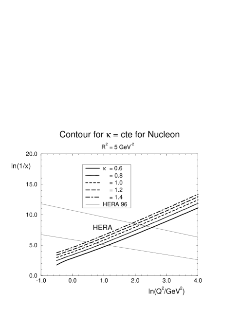
Figure 1: Contour plot for $\kappa=\,cte$ for the GRV 95[4] distribution and $R^{2}=\,5\,GeV^{-2}$. The solid lines show the HERA kinematic region [1].

3. The situation looks even more controversial if we plot the average value of the anomalous dimension, $<\gamma>\,\,=\,\,\partial\ln(xG(x,Q^{2}))/\partial\ln Q^{2}$, in the GRV parameterization. Fig.2 shows two remarkable lines: the line $<\gamma>=1$, where the deep inelastic cross section reaches the value compatible with the geometrical size of the proton; and the line $<\gamma>\,=\,1/2$, which is the characteristic line in which vicinity both the BFKL Pomeron [8] and the GLR equation [5] should take over the DGLAP evolution equations. HERA data passed over the second line and even for sufficiently small values of $Q^{2}$ they crossed the first one without any indication of a strange behaviour near these lines.

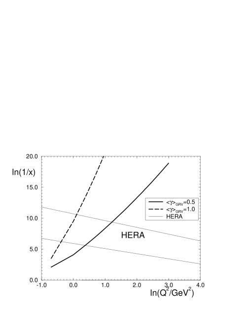
Figure 2: Contours for $<\gamma>$ = 1 and $<\gamma>$ = 1/2 for the GRV95 gluon density and HERA kinematic region.

From the above discussion we conclude that the physical interpretation of HERA data looks controversial and the statement that the DGLAP evolution works is first but not the last outcome of HERA data. We expect also that the SC will be essential in HERA kinematic region. However, to treat the SC we need a more general approach than the GLR one [5], [7], which gave a theoretical approach to the SC only to the right of the critical line $<\gamma>\,=\,\frac{1}{2}$, at large values of $Q^{2}$. In this paper we develop a general approach to the SC, that will allow us to give reliable estimates for the SC in the kinematic region to the left of the line $<\gamma>\,=\,1/2$, i.e., for large $ln(1/x)$ and small $Q^{2}$.

This paper is organized as follows. In section 2 we present the Glauber or Eikonal approach for high energy scattering off nucleon. We discuss the SC for the gluon distribution in a nucleon and for the $F_{2}$ deep inelastic structure function, concentrating mostly on the theory status of this approach and on the predicted scale for the SC. We analyse also the effect of the SC on the $b_{t}$-dependence of the gluon distributions and $F_{2}$, and the consequent approach to the “soft” physics. After a brief discussion, in section 3, of the first correction to the Glauber (Eikonal) approach, we present, in section 4, a new evolution equation that sums all SC diagrams which are of order $(\alpha_{\rm S}\,\ln(1/x)\,\ln Q^{2})^{n}$ and $\kappa^{n}$. This equation is solved for $\alpha_{\rm S}$ constant in the semiclassical approach. The solution is compared with that of the GLR equation [5] and with the Glauber approach. Finally, section 5 summarizes our results.

2 The Eikonal approach in QCD .

2.1 The Mueller formula.

In this section we present the general idea for the Glauber formula in QCD both for the gluon distribution and the $F_{2}$ structure function of DIS. These Glauber formulas will take into account the SC from the eikonalization of the parton-nucleon cross section. The ideas were originally formulated in Refs.[9]-[11].

Let us consider a high energy virtual particle that probes the nucleon gluon distribution ( for example, such a probe could be a virtual graviton or a heavy Higgs boson). In the space-time picture of the process, the virtual probe decays in a gluon-gluon ($GG$) pair, with transverse separation $r_{\perp}$ and the fraction of energy of the probe $z$ and $1-z$, which interacts with the nucleon through a gluon ladder exchange. In high energy (small $x$) limit, $r_{\perp}$ is constant during the interaction for $x\,\,\ll\,\,{1}/(2\,m\,R)$, where $R$ is the target nucleon size. Therefore, the transverse distance $r_{\perp}$ is a good degree of freedom for our problem.

The cross section of the absorption of gluon($G^{*}$) with virtuality $Q^{2}$ and Bjorken $x$ can be written in the form

$$\sigma(\,G^{*}\,)\,\,=\,\,\int^{1}_{0}dz\,\,\int\,\frac{d^{2}r_{\perp}}{\pi}\,\,\int\frac{d^{2}b_{t}}{\pi}|\,\Psi^{G^{*}}_{\perp}(Q^{2},r_{\perp},x,z)\,|^{2}\,\,\sigma_{tot}(GG\,+\,nucleon)\,\,,$$ (2)

where $z$ is the fraction of energy carried by the gluon, $b_{t}$ is the impact parameter and $\Psi^{G^{*}}_{\perp}$ is the wave function of the transverse polarized gluon in the virtual probe. The cross section of the interaction of the $GG$ pair with the nucleon is $\sigma_{tot}(GG\,+\,nucleon)=\sigma(x,r^{2}_{\perp})$. It is important to note that this description is valid in leading log ( $1/x$ ) approximation (LL($1/x$)A), in which only contributions of the order of $(\,\alpha_{\rm S}\ln(\frac{1}{x}\,))^{n}$ were taken into account. In this approximation we can neglect the change of $z$ during the interaction and describe the cross section $\sigma_{tot}(GG\,+\,nucleon)$ as a function of the variable $x$ [5], [12], [13].

The cross section $\sigma(x,r^{2}_{\perp})$ can be written in the form

$$\sigma(x,r^{2}_{\perp})\,\,=\,\,2\,\,\int\,\,d^{2}b_{t}\,\,Im\,a(x,r_{\perp},b_{t})\,\,,$$ (3)

where $a$ is the elastic amplitude for which we have the $s$ - channel unitarity constraint

$$2\,\,Im\,a(x,r_{\perp},b_{t})\,\,=\,\,|a(x,r_{\perp},b_{t})|^{2}\,\,+\,\,G_{in}(x,r_{\perp},b_{t})\,\,,$$ (4)

where $G_{in}$ is the contribution of all inelastic processes. Eq.(4) gives the relation between two unknowns $a$ and $G_{in}$ and has a general solution in the limit of small real part of the elastic amplitude at $x\,\rightarrow 0$

$$a(x,r_{\perp},b_{t})\,\,=\,\,i\,\,\{\,\,1\,\,-\,\,e^{-\,\frac{1}{2}\,\Omega(x,r_{\perp},b_{t})}\,\,\}\,\,,$$ (5)

$$G_{in}(x,r_{\perp},b_{t})\,\,=\,\,1\,\,-\,\,e^{-\,\Omega(x,r_{\perp},b_{t})}\,\,\,\,.$$

The opacity function $\Omega$ has a simple physical meaning, namely $e^{-\Omega}$ is the probability that a $GG$ pair has no inelastic interaction during the passage through the target. $\Omega$ is an arbitrary real function, which can be specified only in a more detailed theory or approach than the unitarity constraint. One of such specific model is the Glauber approach or the Eikonal model.

However, before we discuss this model let us make one important remark on the strategy for the approach to the SC: being able to calculate the opacity $\Omega$ we will have the theory or model for all inelastic processes. Indeed, using AGK cutting rules [15] we can calculate any inelastic process, if we know $\Omega$, in accordance with the $s$-channel unitarity. It is worthwhile mentioning that the inverse procedure does not work. If we know the SC in all details for a particular inelastic process, say for the inclusive production, we cannot reconstruct all other process and the total cross section in particular.

Now, let us built the Glauber approach. First, let us assume that $\Omega$ is small ($\Omega\,\,\ll\,\,1$) and its $b_{t}$ dependence can be factorized as $\Omega\,=\,\widetilde{\Omega}(x,r_{\perp})\,S(b_{t})$ with the normalization $\int\,d^{2}b_{t}\,S(b_{t})\,=\,1$. The factorization was proven for the DGLAP evolution equations [5] and, therefore, all our further calculations will be valid for the DGLAP evolution equations [14] in the region of small $x$ or, in other words, in the Double Log Approximation (DLA) of perturbative QCD (pQCD). Expanding Eq. (5) and substituting it in Eq. (2), one can obtain

$$\sigma_{tot}(x,r_{\perp})\,\,=\,\,\widetilde{\Omega}(x,r_{\perp})\,.$$ (6)

The substitution of Eq. (6) in Eq. (2) gives

$$\sigma(\,G^{*}\,)\,\,=\,\,\int^{1}_{0}dz\,\,\int\,\frac{d^{2}r_{\perp}}{\pi}\,\,|\,\Psi^{G^{*}}_{\perp}(Q^{2},r_{\perp},x,z)\,|^{2}\widetilde{\Omega}(x,r_{\perp})\,\,.$$ (7)

Using Eq. (7) and $\sigma(G^{*})\,\,=\,\,\frac{4\pi^{2}\alpha_{\rm S}}{Q^{2}}\,xG(x,Q^{2})$ as well as the expression for the wave function of the $GG$ pair in the virtual gluon probe ( see Ref.[10] ), one can express $\widetilde{\Omega}(x,r_{\perp})$ through the gluon structure function [9],[10]

$$\widetilde{\Omega}\,\,=\,\,\sigma^{GG}_{N}(x,\frac{r^{2}_{\perp}}{4})\,\,=\,\,\frac{3\,\pi^{2}\,\alpha_{\rm S}}{4}\,\,r^{2}_{\perp}\,xG(x,\frac{4}{r^{2}_{\perp}})\,\,.$$ (8)

The Glauber (eikonal ) approach is the assumption that $\Omega\,=\,\widetilde{\Omega}\,S(b_{t})$ with $\widetilde{\Omega}$ given by Eq. (8) in the whole kinematical region. From the point of view of the structure of the final state, this assumption means that the typical rich inelastic event was modeled as a sum of the diffractive dissociation of the $GG$ pair and uniform in rapidity distribution of produced gluons. For example, we neglected in the Glauber approach all the rich structure of the large rapidity gaps events including the diffractive dissociation in the region of large mass.

Substituting Eq. (8) in Eq. (6) and the result in Eq. (2), and using the wave function $\Psi^{G^{*}}_{\perp}(Q^{2},r_{\perp},x,z)$ calculated in Ref.[10] we obtain the Glauber (Mueller) formula for the gluon structure function

$$xG(x,Q^{2})=\frac{4}{\pi^{2}}\int_{x}^{1}\frac{dx^{\prime}}{x^{\prime}}\int_{\frac{4}{Q^{2}}}^{\infty}\frac{d^{2}r_{\perp}}{\pi r_{\perp}^{4}}\int_{0}^{\infty}\frac{d^{2}b_{t}}{\pi}2\left\{1-e^{-\frac{1}{2}\,\sigma^{GG}_{N}(x^{\prime},\frac{r^{2}_{\perp}}{4})S(b_{t})}\right\}\,.$$ (9)

The first term in the expansion of Eq. (9) with respect to $\sigma^{GG}_{N}$ gives the DGLAP equation in the region of small $x$.

To simplify our calculations we will use the Gaussian parameterization for the profile function $S(b_{t})$, namely

$$S(b^{2}_{t})\,\,=\,\,\frac{1}{\pi\,R^{2}}\,e^{-\,\frac{b^{2}_{t}}{R^{2}}}\,\,.$$ (10)

Using this profile function and integrating over $b_{t}$, we obtain ($N_{c}=N_{f}=3$)

$$xG(x,Q^{2})=\frac{2R^{2}}{\pi^{2}}\int_{x}^{1}\frac{dx^{\prime}}{x^{\prime}}\int^{\frac{1}{Q^{2}_{0}}}_{\frac{1}{Q^{2}}}\frac{dr_{\perp}^{2}}{r_{\perp}^{4}}\left\{\,\,C\,\,+\,\,ln(\kappa_{G}(x^{\prime},r_{\perp}^{2}))\,\,+\,\,E_{1}(\kappa_{G}(x^{\prime},r_{\perp}^{2}))\right\}\,\,,$$ (11)

where $C$ is the Euler constant and $E_{1}$ is the exponential integral (see Ref.[16] Eq. 5.1.11) and

$$\kappa_{G}(x^{\prime},r_{\perp}^{2})=\frac{3\alpha_{\rm S}(\frac{1}{r^{2}_{\perp}})\pi r^{2}_{\perp}}{2R^{2}}x^{\prime}G^{DGLAP}(x^{\prime},\frac{1}{r^{2}_{\perp}})\,\,.$$ (12)

The Eq. (9) is the master equation of this section and it gives a way to estimate the value of the SC.

A similar Glauber (eikonal ) formula may be obtained for the deep inelastic structure function $F_{2}(x,Q^{2})$. In this case, the virtual probe decays into a quark anti-quark pair which interacts with the nucleon trough a gluon ladder exchange. Taking into account $N_{f}$ quark flavours and integrating the quark pair wave function over $z$, we obtain a Glauber formula for $F_{2}$ ( see Refs. [6] [9] [10] )

$$F_{2}(x,Q^{2})\,\,=\,\,\frac{N_{c}}{6\,\pi^{3}}\,\sum^{N_{f}}_{1}\,\,Z^{2}_{f}\,\,\,\int^{\infty}_{\frac{1}{Q^{2}}}\,\frac{dr^{2}_{\perp}}{r^{4}_{\perp}}\,\int\,d^{2}b_{t}\,\,\{\,1\,\,-\,\,e^{-\,\frac{1}{2}\,\Omega_{q\bar{q}}(x,r_{\perp},b_{t})}\,\}\,\,,$$ (13)

where $\Omega_{q\bar{q}}\,\,=\,\sigma^{q\bar{q}}_{N}\,S(b_{t}^{2})\,=\,\frac{4}{9}\Omega$, and $Z_{f}$ is the quark charge fraction. After integration over $b_{t}$ using the Gaussian profile function $S(b_{t})$ one can reduce Eq. (13) to ( $N_{c}=3$ )

$$F_{2}(x,Q^{2})\,\,=\,\,\frac{R^{2}}{2\pi^{2}}\,\sum^{N_{f}}_{1}Z^{2}_{f}\,\int^{\frac{1}{Q^{2}_{0}}}_{\frac{1}{Q^{2}}}\,\,\frac{d\,r^{2}_{\perp}}{r^{4}_{\perp}}\left\{\,\,C\,\,+\,\,ln(\kappa_{q}(x^{\prime},r_{\perp}^{2}))\,\,+\,\,E_{1}(\kappa_{q}(x^{\prime},r_{\perp}^{2}))\right\}\,\,,$$ (14)

with $\kappa_{q}\,\,=\,\,\frac{4}{9}\,\kappa_{G}$.

2.2 Theory status of the Mueller formula.

In this section we shall recall the main assumptions that have been made to obtain the Mueller formula.

1. The gluon energy ($x$) should be high (small) enough to satisfy $x\,\ll\,\frac{1}{mR}$ and     $\alpha_{\rm S}ln(1/x)\leq 1$. The last condition means that we have to assume the leading $ln(1/x)$ approximation of perturbative QCD for the nucleon gluon structure function.

2. The DGLAP evolution equations hold in the region of small $x$ or, in other words, $\alpha_{\rm S}ln(1/r^{2}_{\perp})\leq 1$. One of the lessons from HERA data is the fact that the DGLAP evolution can describe the experimental data.

These two assumptions mean that we describe the gluon emission in Double Log Approximation ( DLA) of perturbative QCD. In other words, we extract from each Feynman diagram of order $\alpha_{\rm S}^{n}$ the contribution of order $(\,\alpha_{\rm S}\,\ln 1/x\,\ln Q^{2}/Q^{2}_{0}\,)^{n}$, neglecting all other contributions of the same diagram. In terms of the DGLAP evolution, we have to assume that the DGLAP evolution equations describe the gluon emission in the region of small $x$. However, the first assumption is very important for the whole picture, since it allows us to treat successive rescatterings as independent and simplifies all formulae reducing the problem to an eikonal picture of the classical propagation of a relativistic particle with high energy ($ER\,\gg\,1$) through the target.

3. Only the fastest partons ($GG$ pairs) interact with the target. This assumption is an artifact of the Glauber approach, which looks strange in the parton picture of the interaction. Indeed, in the parton model we rather expect that all partons, not only the fastest one, should interact with the target. In the next section we will show that corrections to the Glauber approach due to the interaction of slower partons are essential in QCD.

4. There are no correlations (interaction) between partons from the different parton cascades. This assumption means that even the interaction of the fastest $GG$-pair was taken into account in the Mueller formula only approximately and we have to assume that we are dealing with large number of colours to trust the Mueller formula. Indeed, it has been proven that correlations between partons from different parton cascades lead to corrections to the Mueller formula of the order of $1/N^{2}_{c}$, where $N_{c}$ is the number of colours ([18]).

Let us discuss the large $N_{c}$ approximation in more detail. The main principle, used in our large $N_{c}$ approach, has been formulated by Veneziano et al. [17], namely, we sum leading $N_{c}$ diagrams considering $N_{c}\,\alpha_{\rm S}\,\approx\,1$ while $\alpha_{\rm S}\,\,<\,\,1$, separately in each topological configuration. For example, at high energy ( low $x$ ) the main contribution gives the planar diagrams ( see Fig.3a )which lead to the DGLAP evolution equations in leading $\ln(1/x)$ approximation of pQCD. In fact, it has not been proven yet that more complicated planar diagrams such as of Fig.3b could be neglected at high energies, but several simple examples have been considered ( see Ref.[18] ) which show that this hypothesis is very likely ( see review [19] for a detailed discussion on the subject). The two sheet configuration (see Fig.3c) is suppressed since it is proportional to an extra $\alpha_{\rm S}$. The main contribution at high energy in this configuration are the diagrams that has been summed in the Glauber - Mueller approach (see Ref.[18]) in which the smallness of the order of $\alpha_{\rm S}$ is compensated by extra power of $xG(x,Q^{2})$. The actual parameter of the Glauber - Mueller approach is $\kappa$ which could be of the order of 1. However we neglected the contribution of the diagrams of Fig.3d type in which one can see a transition from one two sheet topology to another. As has been shown [18] such transition is suppressed by a factor $\frac{1}{N^{2}_{c}}$. The use of the $\frac{1}{N_{c}}$ expansion can be suspicious in this case, because such transition gives a $\frac{1}{N_{c}^{2}}$ corrections to the anomalous dimension. However, it was shown [25] that $\frac{1}{N_{c}}$ - expansion works quite well, justifying our approach. To be safe we assume that $\frac{\alpha_{\rm S}}{N^{2}_{c}}\,\ln(1/x)\,<\,1$.

Figure 3: Topological configurations for large $N_{c}$ approach: a) ladder diagram; b) general planar diagram; c) Glauber-Mueller approach; d) general two sheet diagram.

5. There are no correlations between different gluons inside the nucleon, of about the same energy, except the fact that they are distributed in the area with radius $R$. This is the main assumption of the Eikonal model which makes this model simple and, of course, it is a great simplification of the unknown ( nonperturbative ) structure of the nucleon. $R$ is the correlation radius for such gluons and the estimates from the HERA data have been discussed in the introduction.

2.3 The modified Mueller formula.

The next step of our approach is to give an estimate of the SC using the Mueller formula. However, before doing so, we have to study how well the DLA of perturbative QCD works, as it was heavily used in the derivation of the Mueller formula. Let us consider the small $x$ limit of the DGLAP evolution equation, which takes a simple form

$$\frac{\partial^{2}xG(x,Q^{2})}{\partial\ln(1/x)\,\partial\ln Q^{2}}\,\,=\,\,\frac{\alpha_{\rm S}\,N_{c}}{\pi}\,xG(x,Q^{2})\,\,.$$ (15)

This expression may be obtained from the full DGLAP equation taking only the DLA limit of the anomalous dimension, namely, $\gamma^{DLA}\,\,=\,\,\frac{\alpha_{\rm S}N_{c}}{\pi}\frac{1}{\omega}$.

In order to estimate numericaly how well the DLA works, we use the GRV parameterization [4] for the nucleon gluon distribution. This parameterization describes all available experimental data quite well, including recent HERA data at low $x$ and low $Q^{2}$ ($Q^{2}\,\geq\,1.5\,GeV^{2}$). Moreover, the GRV parameterization is suited for our purpose because (i) the initial virtuality for the DGLAP evolution is small ($Q_{0}^{2}\approx 0.25\,GeV^{2}$) and we can discuss the contribution of the large distances in the MF having some support from experimental data; (ii) in this parameterization the most essential contribution comes from the region where $\alpha_{s}lnQ^{2}\approx 1$ and $\alpha_{s}ln1/x\approx 1$. This allows the use of the double leading log approximation of pQCD, where the MF is proven [10]. It should be also stressed that we consider the GRV parameterization as a solution of the DGLAP evolution equations, disregarding how much of the SC has been taken into account in this parameterization in the form of the initial gluon distribution.

However, in spite of the fact that the DGLAP evolution in the GRV parameterization starts from very low virtuality ( $Q^{2}_{0}\,\sim\,0.25\,GeV^{2}$) it does not reach the DLA in the accessible kinematic region ($Q^{2}\,>\,1\,GeV^{2},\,x\,>\,10^{-5}$). To illustrate this statement we plot in Fig.4 the ratio:

$$\frac{<{\alpha_{\rm S}}>^{GRV}}{\alpha_{\rm S}}\,\,=\,\,\frac{\frac{\partial^{2}xG^{GRV}(x,Q^{2})}{\partial\ln(1/x)\,\partial\ln Q^{2}}}{\frac{\alpha_{\rm S}N_{c}}{\pi}xG^{GRV}(x,Q^{2})}\,\,.$$

This ratio is equal to 1 if the DLA holds. From Fig.4 one can see that this ratio is rather around 1/2 even at large values of $Q^{2}$.

Figure 4: The ration $\frac{<\alpha_{\rm S}>^{GRV}}{\alpha_{\rm S}}$ for different values of $Q^{2}$ in the GRV95 parameterization.

We can understand why the corrections to the DLA are so big modeling the small $x$ anomalous dimension $\gamma$ by a simple formula [26]

$$\gamma(\omega)\,\,=\,\,\frac{\alpha_{\rm S}N_{c}}{\pi}\,\{\,\,\frac{1}{\omega}\,\,-\,\,1\,\,\}\,\,,$$ (16)

which has the correct DLA limit at small $\omega$ and satisfies the momentum conservation constraint $\gamma(\omega=1)\,=\,0$. The typical values of $\omega$ in all available parameterizations, even in the GRV, which is the closest one to the DLA, is $<\omega>\,\approx\,0.5$. Therefore, there is about 50% correction to the DLA, meaning it cannot provide reliable estimates for the gluon structure function.

On the other hand, our master equation (see Eq. (9)) is proven in DLA. Willing to develop a realistic approach in the region of not ultra small $x$ ($x\,>\,10^{-4})$ we have to change the master equation ( Eq. (9) ). We suggest to substitute the full DGLAP kernel in the first term of the r.h.s, which gives

$$xG(x,Q^{2})\,\, = \,\,xG(x,Q^{2})(\,{Eq.~{}(\ref{MF})}\,)\,\,+\,\,xG^{DGLAP}(x,Q^{2})\,\,$$ (17)

$$- \,\,\frac{\alpha_{\rm S}N_{c}}{\pi}\,\int^{1}_{x}\,\int^{Q^{2}}_{Q^{2}_{0}}\,\,\frac{dx^{\prime}}{x^{\prime}}\,\frac{dQ^{\prime 2}}{Q^{\prime 2}}\,x^{\prime}G^{DGLAP}(x^{\prime},Q^{\prime 2})\,\,.$$

The above equation includes $xG^{DGLAP}(x,Q^{2}_{0})$ as the initial condition for the gluon distribution and gives $xG^{DGLAP}(x,Q^{2})$ as the first term of the expansion with respect to $\kappa_{G}$. Therefore, this equation is an attempt to include the full expression for the anomalous dimension for the scattering off each nucleon, while we use the DLA to take into account all SC. Our hope, which we will confirm by numerical calculation, is that the SC are small enough for $x\,>\,10^{-3}$ and we can be not so careful in the accuracy of their calculation in this kinematic region. Going to smaller $x$, the DLA becomes better and Eq. (17) tends to the master equation (9).

We suggest an analogous improvement in the calculation of the SC correction for the structure function $F_{2}$. We subtract the Born term of Eq. (14) and add the DGLAP evolved structure function $F_{2}^{DGLAP}$. The result reads

$$F_{2}(x,Q^{2})=F_{2}^{SC}-F_{2}^{BORN}+F_{2}^{DGLAP}\,,$$ (18)

where $F_{2}^{SC}$ is given by Eq. (14), and the Born term is given by

$$F_{2}^{BORN}(x,Q^{2})=\frac{1}{2\pi}\,\sum^{N_{f}}_{1}\,\,\alpha_{\rm S}\,Z^{2}_{f}\,\,\int^{\ln Q^{2}}_{\ln Q^{2}_{0}}\,\frac{2}{3}d(\ln Q^{\prime 2})xG^{DGLAP}(x,Q^{\prime 2})\,\,.$$ (19)

As discussed above, $F_{2}^{DGLAP}(x,Q^{2}_{0})$ is the initial condition for $F_{2}$ and $F_{2}^{DGLAP}(x,Q^{2})$ is the first term of the expansion with respect to $\kappa_{q}$. Now, we are able to evaluate the amount of SC in the nucleon gluon distribution and in the $F_{2}$ structure function predicted by the eikonal approach.

2.4 The gluon structure function for nucleon.

Before performing calculations we would like to discuss which observable we are able to calculate using the Mueller formula. One can see from Eq.(9) that the large distances enter into this formula. In spite of the fact that this formula provides the infrared safe answer, or in other words, the integral is finite in the region of the large distances, we cannot trust our calculations in this region since we have no arguments to apply pQCD in this kinematic region. Therefore, first we need to indroduce a scale of distances for which we can trust the pQCD calculations. We decided to choose the value of $r^{2}_{\perp\,0}\,\,=\,\,1\,GeV^{-2}$ as such scale. The argument comes from the new HERA data on the deep inelastic structure function $F_{2}(x,Q^{2})$ [1] which show that the GRV parameterization works quite well starting from $Q^{2}\,\,\geq\,\,1\,GeV^{2}$. Therefore, we consider the GRV structure functions at $Q^{2}\,=\,1\,GeV^{2}$ both for gluons and quarks, as a lucky guess of the initial conditions for the QCD evolution that takes into account the unknown nonperturbative large distance physics, disregarding all physical motivation for such a guess. We believe that such a choice give us a reliable estimate of the SC which stem from small distances, being on the theoretical control of pQCD. In the following calculations we will use a fixed value for the QCD running coupling constant, $\alpha_{\rm S}\,=\,0.25$.

In order to evaluate quantitatively the influence of the SC on the evolution of gluon structure function we calculate three functions

$$R_{1}\,=\,\frac{xG(x,Q^{2})}{xG^{GRV}(x,Q^{2})}\,\,,$$ (20)

$$<\omega>\,\,=\,\,\frac{\partial\ln(xG(x,Q^{2}))}{\partial\ln(1/x)}\,\,,$$ (21)

and

$$<\gamma>\,\,=\,\,\frac{\partial\ln(xG(x,Q^{2}))}{\partial\ln(Q^{2}/Q^{2}_{0})}\,\,.$$ (22)

We chose these functions because, in the semiclassical approach ( see Ref. [5] ), the gluon structure function has a general form

$$xG(x,Q^{2})\,\,=\,\,C\,\{Q^{2}\}^{<\gamma>}\,\,\{\frac{1}{x}\}^{<\omega>}\,\,,$$ (23)

where we expect the exponents to be smooth functions of $ln(\frac{1}{x})$ and $ln(Q^{2})$. We will see a posteriori that, indeed, $<\omega>$ and $<\gamma>$ turn out to be smooth functions in the region of small $x$. All functions in Eq. (20) - Eq. (22) have transparent physical meaning. Indeed, the function $<\gamma>$ is the average anomalous dimension in DIS, the function $<\omega>$ is the intercept of so called “hard” Pomeron while function $R_{1}$ is equal to $1/N_{Pomeron}$, where $N_{Pomeron}$ is the average number of “hard” Pomerons taking part in the rescatterings . “Hard” Pomeron in our approach is $xG(x,\frac{1}{r^{2}_{\perp}})$ in Eq. (9) ($\,(xG(x,\frac{1}{r^{2}_{\perp}}))^{n}$ corresponds to $n$ - Pomeron exchange). Indeed, due to the AGK cutting rules [15], which have been proven in QCD in Ref. [27], the inclusive cross section is proportional to the exchange of one Pomeron or, in other words, only the first term in Eq. (9) contributes to the inclusive cross section of particles in the central region of rapidity ($\sigma_{incl}=\frac{dN}{dy}$). On the other hand, $\sigma_{incl}\,=\,N\,\sigma_{tot}$, where $N$ is the average multiplicity and $\sigma_{tot}$ is the total cross section given by Eq. (9). $N$ is equal to $N_{Pomeron}N(one\,\,Pomeron\,\,exchange)$, where $N(one\,\,Pomeron\,\,exchange)\,\,=\,\,\frac{1}{\sigma_{Pomeron}}\frac{d\sigma_{Pomeron}}{dy}$. Noticing that $\sigma_{Pomeron}$ is the first term in Eq. (9), we obtain that $N_{Pomeron}\,=\,\frac{1}{R_{1}}$.

In Fig.5, we show the values of $R_{1}$ as a function of $y=ln(1/x)$ for different values of the virtuality $Q^{2}$ and two values of $R^{2}$. The figure illustrates the general feature of the SC in the eikonal model: the distribution $xG$ is strongly suppressed as $y$ increases ( $x$ tends to zero). In HERA kinematic region, $2\,<\,y\,<\,10$ and $Q^{2}=2.5\,\,GeV^{2}$, the modified Mueller formula for $R^{2}=10\,\,GeV^{-2}$ predicts a suppression that varies from less then $1\%$ up to $10\%$. For $Q^{2}=20\,\,GeV^{2}$, the suppression varies from less then $1\%$ up to $13\%$. This effect is even bigger for smaller value of $R^{2}$. For example, for $R^{2}=5\,\,GeV^{-2}$ and $Q^{2}=2.5\,\,GeV^{2}$, the suppression goes from less then $1\%$ for $y=2$ to almost $15\%$ for $y=10$. For $Q^{2}=20\,\,GeV^{2}$, the suppression goes from less then $1\%$ for $y=2$ to $22\%$ for $y=10$.

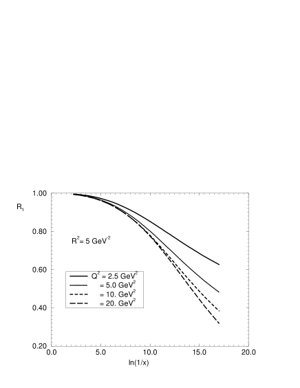
Figure 5: $R_{1}$ ratio as a function of $y=ln(1/x)$ and $Q^{2}$ for two values of $R^{2}$.

We can interpretate the result shown in Fig.5 in a different way saying that the average number of the “hard” Pomerons participating in rescattering changes from 1 at $x=10^{-2}$ to 1.25 ($R^{2}=10\,GeV^{-2}$ and $Q^{2}\,=\,10\,\,GeV^{2}$) or 1.43 ($R^{2}=5\,GeV^{-2}$) at $x\rightarrow 10^{-5}$.

In Fig.6 are shown the results for $<\omega>$ as a function of $y$ for several values of $Q^{2}$ and two values of $R^{2}$. As we can see, the values of $\omega$ are softened by the SC when compared with the GRV values.

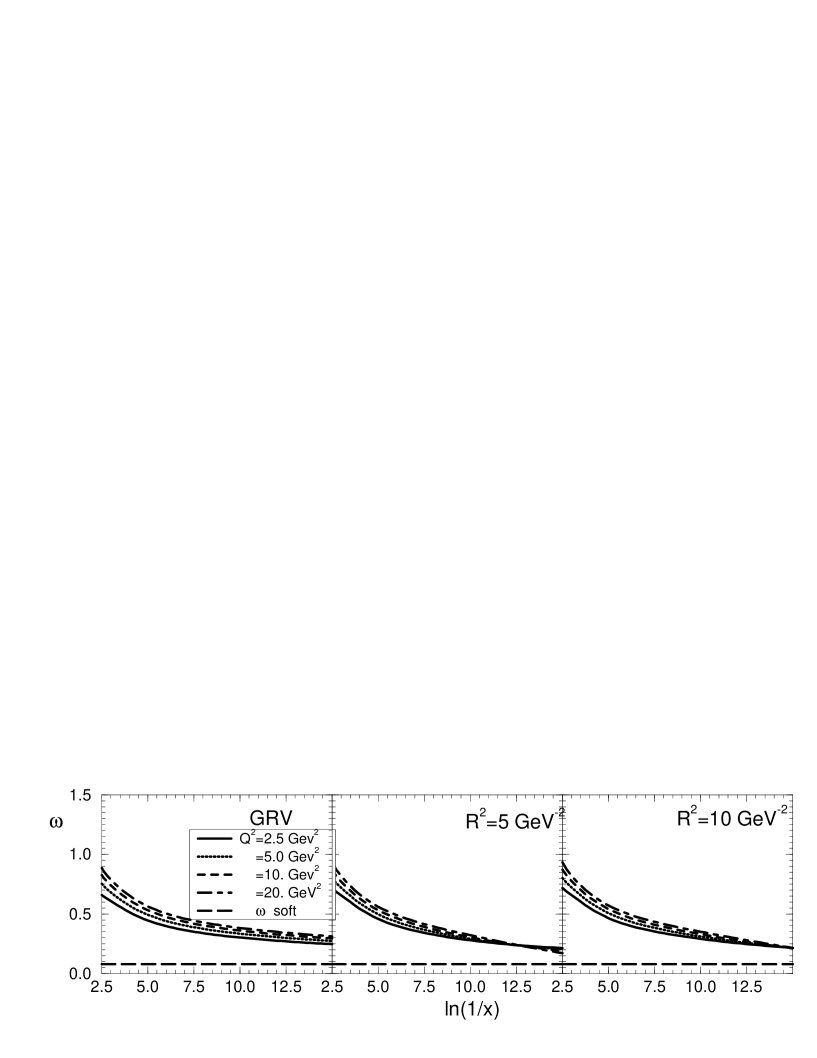
Figure 6: The values of $<\omega>$ as a function of $y=ln(1/x)$ and $Q^{2}$ for GRV and two values of $R^{2}$. It is also plotted the soft Pomeron intercept $\omega\,=\,0.08$.

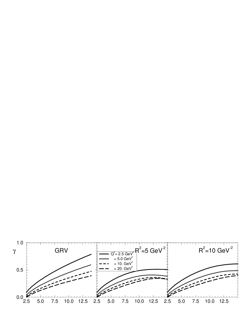
Figure 7: The values of $<\gamma>$ as a function of $y=ln(1/x)$ and $Q^{2}$ for GRV and two values of $R^{2}$.

In Fig.7 are shown the results for $<\gamma>$ calculated from expression (22). The values of $<\gamma>$ suffer a strong suppression as compared to the GRV ones. It means that the $Q^{2}$ evolution of the gluon distribution is significantly modified by the SC.

The figures 5, 6 and 7 also illustrate the dependence of SC on the value of $R^{2}$. For example, for $R^{2}\,\,=\,\,10\,GeV^{-2}$, the SC, generated by the eikonal approach, suppress the value of $\omega$, but the value of the SC is not enough to provide a match between the “soft” and “hard” processes. To illustrate this point we put in Fig.6 the intercept of the so called “soft” Pomeron $\omega_{soft}\,=\,0.08$ [28]. For $R^{2}\,\,=\,\,5\,GeV^{-2}$, the suppression is bigger, but $\omega$ does not reach the “soft” Pomeron intercept. However, for $Q^{2}\,=\,20\,GeV^{2}$ sufficiently small values of $x$ ($y\approx 20$) and $Q^{2}\,=\,20\,GeV^{2}$, the SC reduces the values of $\omega$ reaching the “soft” Pomeron intercept. One can see that $<\omega>$ turns out to be bigger than this intercept at small values of $Q^{2}$. It occurs because these values of $Q^{2}$ are close to the initial condition and do not generate enough shadowing.

As we have discussed the SC in the eikonal approach considerably reduce the value of $<\gamma>$. For $R^{2}\,=\,5\,\,GeV^{-2}$, the mean value of the anomalous dimension $<\gamma>$ reaches the value $\frac{1}{2}$ only for $Q^{2}\,=\,2.5\,GeV^{2}$ in the range $10\,<\,y\,<\,16$. For $Q^{2}\,>\,2.5\,GeV^{2}$, $<\gamma>$ is always less then $\frac{1}{2}$. Thus we expect that the BFKL Pomeron will not be seen in the deep inelastic gluon structure function at least in HERA kinematic region. For $R^{2}\,=\,10\,\,GeV^{-2}$, however, the strength of the SC is such that $<\gamma>\,\,>\,\,\frac{1}{2}$ in the accessible kinematic region. It means that, for $Q^{2}\,\leq\,2.5\,\,GeV^{2}$ and $7.5\,<\,y$, the BFKL Pomeron could give a visible contribution. The above discussion illustrates the role of SC and the $R^{2}$ parameter on the transition to the BFKL dynamics which we are going to discuss a bit later in more details.

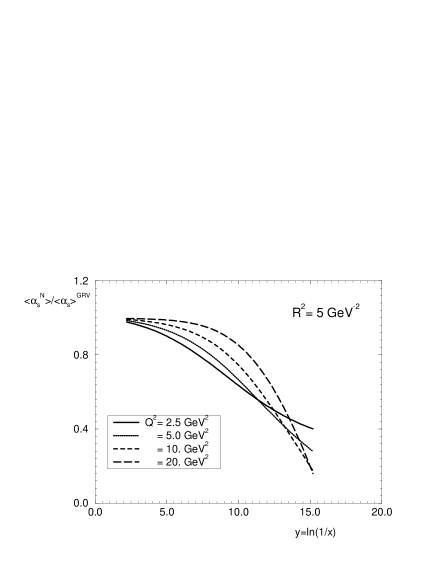
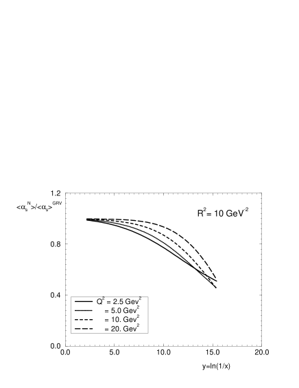
Figure 8: The values of the effective $\alpha_{\rm S}$ in the parton cascade with SC.

In order to complete the discussion of the SC from Mueller formula, we plot in Fig.8 the expression

$$\frac{<\alpha_{\rm S}^{N}>}{<\alpha_{\rm S}>^{GRV}}=\frac{xG^{GRV}(x,Q^{2})}{xG_{N}(x,Q^{2})}\frac{\left[\frac{\partial}{\partial\ln\frac{1}{x}\partial\ln Q^{2}}(xG_{N}(x,Q^{2}))\right]}{\left[\frac{\partial}{\partial\ln\frac{1}{x}\partial\ln Q^{2}}(xG^{GRV}(x,Q^{2}))\right]}\,,$$ (24)

which is the ratio of the effective $\alpha_{\rm S}$ in DLA with and without the SC. In some sense this is the effective value of the QCD coupling constant in the parton cascade with SC, and characterizes the amount of shadowing taken into account in the DGLAP evolution of the gluon distribution. The results present a weakening of the effective coupling constant which accepts a simple interpretation. In the small-$x$ region, the gluon density increases and in a typical parton cascade cell there are many partons with different colors. The color average gives smaller mean color charge at large gluon densities and $<\alpha_{\rm S}>$ is reduced. From the figure we can see that SC modify the DGLAP evolution for a large kinematic region, even for $Q^{2}\geq 10\,\,GeV^{2},$ though including a substantial part of HERA data.

2.5 The DIS structure function $F_{2}$.

In this section we evaluate the SC predicted by the Glauber approach for $F_{2}$. We calculate $F_{2}$ from the modified Mueller formula (18)

$$F_{2}(x,Q^{2})=F_{2}^{SC}-F_{2}^{BORN}+F_{2}^{DGLAP}\,,$$

where $F_{2}^{SC}$ and $F_{2}^{BORN}$ are given by Eq. (14) and Eq. (19) respectively. We calculate $F_{2}^{DGLAP}$ from the GRV 95 [29] distribution $u$, $d$, $s$ and $xG$ using the expression

$$F_{2}^{DGLAP}(x,Q^{2})=\sum_{u,d,s}\,\epsilon_{q}^{2}\,x[q(x,Q^{2})+\bar{q}(x,Q^{2})]+F_{2}^{c}(x,Q^{2},m_{c}^{2})\,,$$ (25)

where $q$ and $\bar{q}$ represent the light quarks distributions. $F_{2}^{c}$ describes the heavy flavour contribution to $F_{2}$ (disregarding bottom contribution). In this scheme the heavy quarks are not considered as intrinsic partons in the Renormalization Group evolution, but are produced, in LO of perturbation theory, by the gluon-$\gamma^{*}$ fusion process. Thus, the charm component $F_{2}^{c}$ will be generated perturbatively from the intrinsic gluon distribution.

In Fig.9 we plot $F_{2}$ using the full DGLAP evolution, given by Eq. (25), and the modified Mueller formula (18) to take into account the SC. The $F_{2}^{c}$ component was calculated from the gluon distribution in LO, as described in Ref.[29]. The SC are not included in the gluon distribution that enter in the $F_{2}^{c}$ calculation. We expect that it would give a correction for $F_{2}$ smaller then the correction given by Eq. (18), at least by a factor $\alpha_{\rm S}(4m_{c}^{2})$.

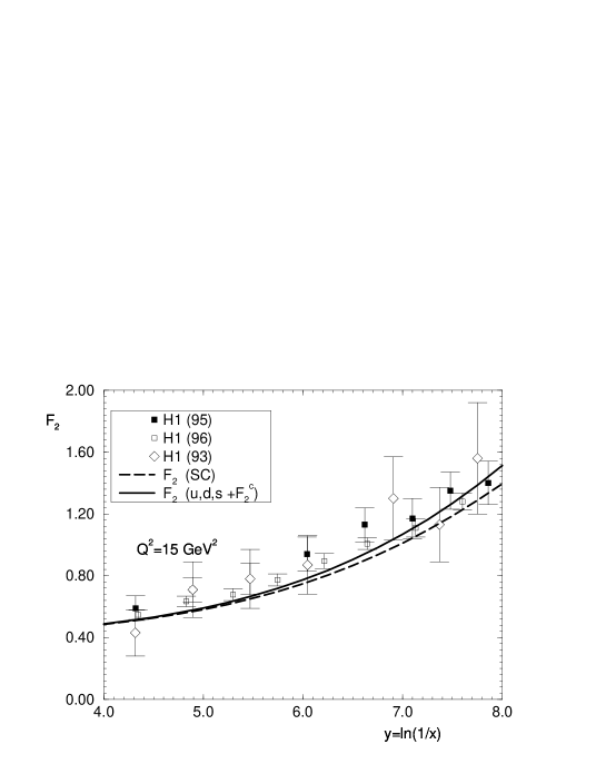
Figure 9: $F_{2}$ calculated from (18) for $Q^{2}_{0}\,=\,1.0\,\,GeV^{2}$.

In figs.(10) and (11) we present the calculation of $F_{2}^{DGLAP}$ and $F_{2}$ given by Eq. (18) as a function of $x$ for different values of $Q^{2}$. The results are compared with H1 96 data. As we can see from the figures, the SC are small for $Q^{2}\,=\,1.5\,GeV^{2}$ since it is very close to the initial value $Q^{2}_{0}\,=\,1\,GeV^{2}$. When $Q^{2}$ grows from $Q^{2}\,=\,1.5\,GeV^{2}$ to $Q^{2}\,=\,6\,GeV^{2}$, the SC increase. For $Q^{2}\,>\,6\,GeV^{2}$, the SC start to fall down again. In fact, the figures show the amount of shadowing that we would expect to be present in the experimental data, if the Glauber approach is supposed to be correct. We conclude that the contribution of the SC to $F_{2}(x,Q^{2})$, predicted from the eikonal approach are rather small in HERA kinematic region unlike the case of the gluon structure function that has been discussed in the previous section. This is an explanation why we are able to describe the HERA experimental data on $F_{2}(x,Q^{2})$ in the GLAP evolution, without taking into account SC in spite of the fact that parameter $\kappa$ is rather big. It turns out the story of the SC contribution is the story about the gluon densities for which we have no independent experimental information. The value of $R_{1}$ for $xG(x,Q^{2})$ is rather big, as we have discussed, but it is still smaller than uncertainties in the values of $xG(x,Q^{2})$ from different attempts ( GRV, MRS and CTEQ) to describe the experimental HERA data in the framework of the DGLAP evolution, that exist on the market.

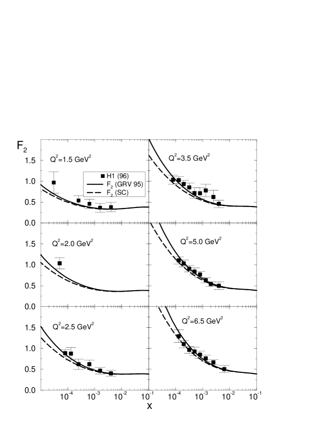
Figure 10: $F_{2}$ calculated from (18) for $Q^{2}_{0}\,=\,1.0\,\,GeV^{2}$ compared with H196 data[1].

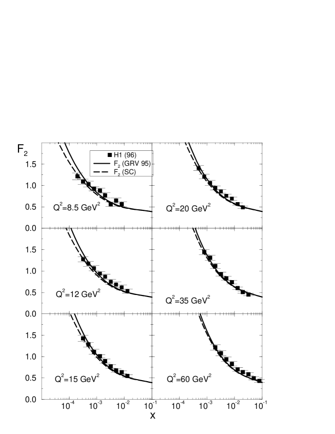
Figure 11: $F_{2}$ calculated from (18) for $Q^{2}_{0}\,=\,1.0\,\,GeV^{2}$ compared with H196 data[1].

2.6 The $b_{t}$ dependence of the gluon distribution.

In the next two subsections we will investigate how the SC work at different values of the impact parameter $b_{t}$. We hope, that the impact parameter distribution will help us to understand better the matching between “soft” and “hard” interactions. In order to do this we introduce the function $xG(x,Q^{2},b_{t})$ defined by the normalization

$$\int\,\,d^{2}\,b_{t}\,\,xG(x,Q^{2},b_{t})\,\,=\,\,xG(x,Q^{2})\,\,,$$ (26)

where $xG(x,Q^{2})$ is the gluon distribution in perturbative QCD. We introduce also the function $xG(x,Q^{2},t)$ given by

$$xG(x,Q^{2},t)\,\,=\,\,\int\,d^{2}b_{t}e^{i\,\vec{q}_{t}\cdot\vec{b}_{t}}\,\,xG(x,Q^{2},b_{t})\,\,.$$ (27)

where $t$ is the momentum transfer $t=-q^{2}_{t}$.

In the DGLAP evolution equation, the $b_{t}$ dependence can be factorized out in the form [5]

$$xG(x,Q^{2},b_{t})\,\,=\,\,xG(x,Q^{2})\,S(b_{t})\,\,,$$ (28)

where the profile function $S(b_{t})$ is related to the two gluon nucleon form factor $F(t)$ as

$$F(t)\,\,=\,\,\int\,d^{2}b_{t}e^{i\,\vec{q}_{t}\cdot\vec{b}_{t}}\,\,S(b_{t})\,\,.$$ (29)

If we consider the exponential parameterization of the profile function $S(b_{t})$, Eq.( 28) and (29) give also an exponential $t$- dependence for the gluon structure function, which can be obtained by the ratio

$$\frac{xG(x,Q^{2},t)}{xG(x,Q^{2},t=0)}\,\,=\,\,F(t)\,\,=\,\,e^{-\frac{R^{2}}{4}\,|t|}\,\,.$$ (30)

Thus the DGLAP evolution predicts a slope $B\,\,=\,\,\frac{R^{2}}{4}$, that does not depend on $x$ and $Q^{2}$.

However, as we will show, the SC will lead to an $x$ and $Q^{2}$- dependence of the $B$ slope, as well as a non factorizable $b_{t}$ - dependence of the gluon structure function.

We introduce the impact parameter $b_{t}$ dependent function $xG(x,Q^{2},b_{t})$ defined by Eq. (26), where $xG(x,Q^{2})$ is the gluon distribution given by the Glauber formula (9). From (26), $xG(x,Q^{2},b_{t})$ can be written as

$$xG(x,Q^{2},b_{t})\,\,=\,\,\frac{2}{\pi^{3}}\,\,\int^{1}_{x}\,\frac{d\,x^{\prime}}{x^{\prime}}\,\,\int^{\infty}_{\frac{1}{Q^{2}}}\,\,\frac{d\,r^{2}_{\perp}}{r^{4}_{\perp}}\,\,\{\,\,1\,\,-\,\,e^{-\,\frac{1}{2}\sigma^{GG}_{N}\,S(b_{t})}\,\,\}\,\,,$$ (31)

where $\sigma^{GG}_{N}$ was defined in Eq. (8). Following the discussion before Eq. (17) we will modify Eq. (31) in order to use the full DGLAP kernel to describe the gluon-nucleon interaction and the DLA to take into account the SC. We add a term proportional to the gluon distribution and subtract the Born term of (31). This procedure gives

$$xG(x,Q^{2},b_{t})\,\,=\, \,xG^{DGLAP}(x,Q^{2})S(b_{t})+xG(x,Q^{2},b_{t})(\ref{BMF})$$ (32)

$$- \frac{2}{\pi^{3}}\,\,\int^{1}_{x}\,\frac{d\,x^{\prime}}{x^{\prime}}\,\,\int^{\infty}_{\frac{1}{Q^{2}}}\,\,\frac{d\,r^{2}_{\perp}}{r^{4}_{\perp}}\,\,\,\frac{1}{2}\sigma^{GG}_{N}\,S(b_{t})\,.$$

This expression keeps the same $b_{t}$ dependence in the Born term and gives the correct match with Eq. (26). In all calculations we use a fixed value for the coupling constant $\alpha_{\rm S}=0.25$ and put $Q_{0}^{2}\,=\,1\,GeV^{2}$.

In order to investigate the general properties of the $b_{t}$ dependent distribution, we calculate all the three functions $R_{1}$ (Eq. (20)), $<\omega>$ (Eq. (21)) and $<\gamma>$ (Eq. (22)) using the above expression for $xG(x,Q^{2},b_{t})$ instead of $xG(x,Q^{2})$. The results are plotted in Fig. 12 for $b_{t}\,=\,0$. We can see from the figure that the SC are bigger for the $b_{t}^{2}\,=\,0$ case when compared to the $b_{t}^{2}$ integrated results. The correction term in (32) will be proportional to $\{1-\,\kappa_{G}-exp(-\kappa_{G})\}$, which is bigger then the nonlinear term of Eq. (17).

It is interesting to notice that at $b_{t}$ = 0 the SC give $<\omega>$ approaching $\omega_{soft}$ = 0.08 for $y\,\approx\,14$, which corresponds to $x\,=\,10^{-7}$. Thus we may expect eventually a matching of the DIS data with the “soft” processes at this very small value of $x$.

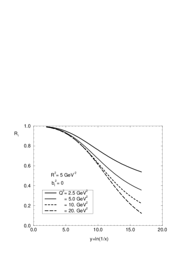
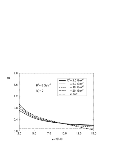
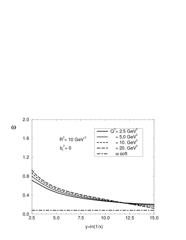
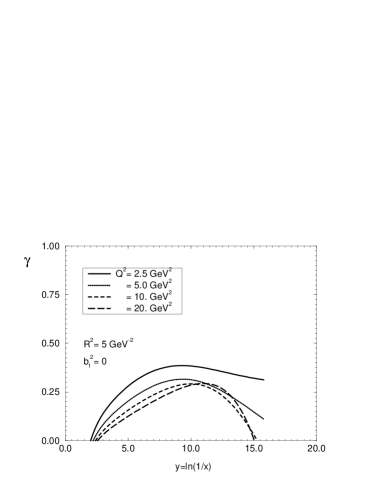
Figure 12: $R_{1}$( Eq. (20)), $\omega$ (Eq. (21)) and $\gamma$(Eq. (22)) function calculated from expression (32) with $b_{t}^{2}\,=\,0$. The results are plotted as functions of $y$ for different values of $Q^{2}$.

The $b_{t}$ dependence of the gluon distribution is illustrated also in Fig.13, which shows $xG(x,Q^{2},b_{t})$ normalized to $b_{t}\,=\,0$ at different values of $x$, $Q^{2}$ and $R^{2}\,=\,5\,GeV^{-2}$. Due to the SC, the width of the $b_{t}$ - distribution becomes bigger with respect to the exponential profile function, and presents an $x$ and $Q^{2}$ dependence. Comparing Fig.(13a) and Fig.(13b), we can see that for smaller values of $x$, where SC are bigger, the $Q^{2}$ dependence of the width is stronger, which leads to a broadening of the $b_{t}$ profile. This effect reflects the $x$ and $Q^{2}$ dependence of the mean squared radius of the interaction $<b^{2}_{t}>$, defined by

$$<b^{2}_{t}>\,\,=\,\,\frac{\int\,\,b^{2}_{t}\,\,d^{2}\,b_{t}\,\,xG(x,Q^{2},b_{t})}{\int\,\,d^{2}\,b_{t}\,\,xG(x,Q^{2},b_{t})}\,\,=\,\,\frac{\int\,\pi\,b^{2}_{t}\,\,d\,b^{2}_{t}\,\,xG(x,Q^{2},b_{t})}{xG(x,Q^{2})}\,.$$ (33)

In Fig.14$,<b^{2}_{t}>$ is plotted for different values of $x$, $Q^{2}$ and $R^{2}$. Due to the SC, $<b^{2}_{t}>$ increases as SC increase, i.e., for $x\,\rightarrow\,0$. In HERA kinematic region, even for $R^{2}\,=\,5\,GeV^{-2}$, $<b^{2}_{t}>$ increases smoothly.

This result should be compared with the expectations for the soft Pomeron exchange. For the soft Pomeron, the slope $B$ is equal to $B\,\,=\,\,B_{0}\,\,+\,\,\alpha^{\prime}_{P}\,\,\ln(1/x)$, where $\alpha^{\prime}_{P}$ does not depend on $Q^{2}$ being $\alpha^{\prime}_{P}\,=\,$ 0.25 $GeV^{-2}$ [28]. We parameterize the behaviour of $<b^{2}_{t}>$ as a straightline for $5\,<\,y\,<\,10$, $<b^{2}_{t}>\,\,=\,\,4B(y\,=\,5)\,\,+\,\,4\alpha^{\prime}_{eff}\,\,\ln(1/x)$. From Fig.14, we can conclude that $\alpha^{\prime}_{eff}$ shows a $Q^{2}$ dependence unlike for the soft Pomeron and its value is rather small both for $R^{2}\,=\,5\,GeV^{-2}$ and $R^{2}\,=\,10\,GeV^{-2}$. Indeed, $\alpha^{\prime}_{eff}\,\,\approx\,\,0.015\,GeV^{-2}\,\,\approx\,\,\frac{1}{16}\,\alpha^{\prime}_{P}$ for $Q^{2}$ = 2.5 $GeV^{2}$ and $\alpha^{\prime}_{eff}\,\,\approx\,\,0.028\,GeV^{-2}\,\,\approx\,\,\frac{1}{9}\,\alpha^{\prime}_{P}$ for $Q^{2}$ = 20 $GeV^{2}$ and $R^{2}$ = 5 $GeV^{-2}$. This straight line approximation is not valid if we go beyond HERA kinematic region.

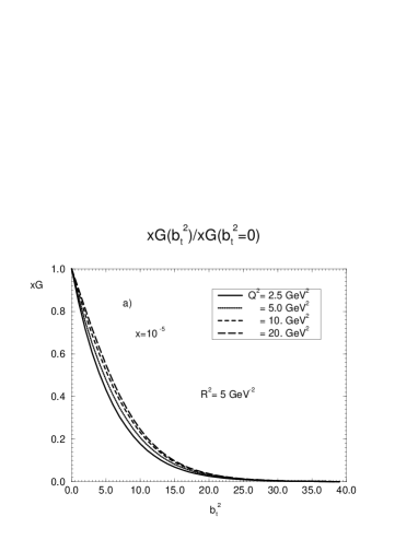
Figure 13: The values of $xG(x,Q^{2},b_{t})$ normalized at $b_{t}^{2}\,=\,0$ as functions of $b_{t}$ for different values of $x$, $Q^{2}$ and $R^{2}\,=\,5\,GeV^{-2}$.

Figure 14: The mean radius of the interaction $<b_{t}^{2}>$ for $xG$ (Eq. (33)).

2.7 The $b_{t}$ dependence of the eikonal $F_{2}$ structure function.

Here we will investigate the $x$ and $Q^{2}$ dependence of the slope $B$ as in the previous subsection, for the $F_{2}$ structure function. We define the modified $b_{t}$ dependent $F_{2}$ structure function as

$$F_{2}(x,Q^{2},b_{t})=F_{2}^{SC}(x,Q^{2},b_{t})-F_{2}^{BORN}(x,Q^{2},b_{t})+F_{2}^{DGLAP}(x,Q^{2},b_{t})\,.$$ (34)

Each term in the above expression obeys the normalization condition

$$F_{2}(x,Q^{2})=\int d^{2}\,b_{t}\,F_{2}(x,Q^{2},b_{t})\,.$$ (35)

The first term in Eq.(34) is the $b_{t}$ dependent Mueller formula

$$F_{2}^{SC}(x,Q^{2},b_{t})=\frac{1}{3\pi^{3}}\int^{Q^{2}}_{Q_{0}^{2}}dQ^{\prime 2}\{1-e^{-\,\frac{1}{2}\,\Omega(x,Q^{\prime 2},b_{t})}\}\,,$$ (36)

where [6]

$$\Omega(x,Q^{\prime 2},b_{t})=\frac{4\alpha_{\rm S}\pi^{2}}{3Q^{\prime 2}}xG(x,Q^{\prime 2})S(b_{t})\,,$$ (37)

and $S(b_{t})$ is the profile function. The Born term for the SC is written as

$$F_{2}^{BORN}(x,Q^{2},b_{t})=\frac{2}{9\pi}\,\sum^{N_{f}}_{1}\,\alpha_{\rm S}\,Z^{2}_{f}\,\,\int^{\ln Q^{2}}_{\ln Q^{2}_{0}}\,d(\ln Q^{\prime 2})xG^{DGLAP}(x,Q^{\prime 2})\,S(b_{t})\,\,.$$ (38)

The $b_{t}$ dependent DGLAP evolved $F_{2}$ is given by (see Eq. (28))

$$F_{2}^{DGLAP}(x,Q^{2},b_{t})=F_{2}^{DGLAP}(x,Q^{2})S(b_{t})\,,$$ (39)

where $F_{2}^{DGLAP}(x,Q^{2})$ is calculated from the GRV distributions for valence, sea, and charm components as already discussed in the $F_{2}$ section (Eq. (25)). All the above expressions for $F_{2}$ fullfill the normalization (35).

In Fig.15 we show the $b_{t}$ dependence of $F_{2}(x,Q^{2},b_{t})$ normalized to $b_{t}\,=\,0$ at different values of $x$, $Q^{2}$ and $R^{2}=5\,GeV^{-2}$. At low values of $x$, the SC lead to a broadening of the $b_{t}$ profile, but the effect is less pronounced when compared to the $b_{t}$ profile of the gluon distribution.

Figure 15: The values of $F_{2}(b_{t}^{2})$ normalized at $b_{t}^{2}\,=\,0$.

We calculate also the mean radius $<\,b_{t}^{2}\,>$ for the $F_{2}$ structure function, which is given by the expression

$$<\,b_{t}^{2}\,>=\frac{\int d\,b_{t}^{2}\,\,b_{t}^{2}\,\,F_{2}(x,Q^{2},b_{t}^{2})}{\int d\,b_{t}^{2}\,\,F_{2}(x,Q^{2},b_{t}^{2})}\,.$$ (40)

The results are plotted in Fig.16. One can see that the effect of the SC on the value of $<b^{2}_{t}>$ is smaller in the $F_{2}$ case then in the $xG$ case. From Fig. 16 one can calculate the value of $\alpha^{\prime}_{eff}$ which is equal $\alpha^{\prime}_{eff}\,\,\approx\,\,0.015\,GeV^{-2}\,\,\approx\,\,\frac{1}{16}\alpha^{\prime}_{P}$ for $Q^{2}\,=\,2.5\,GeV^{2}$ and $\alpha^{\prime}_{eff}\,\,\approx\,\,0.017\,GeV^{-2}$ for $Q^{2}\,=\,20\,GeV^{2}$. Comparing with $\alpha^{\prime}_{eff}$ calculated from the gluon distribution, we conclude that $\alpha^{\prime}_{eff}$ for $F_{2}$ presents a less pronouced $Q^{2}$ dependence.

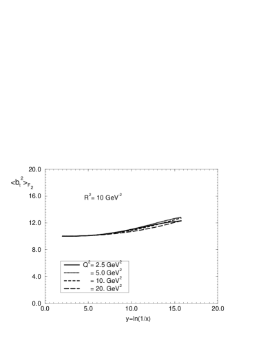
Figure 16: The mean radius of the interaction $<b_{t}^{2}>$ calculated using $F_{2}$(Eq. (34) as a weight function ( Eq. (40)).

2.8 Energy sum rules.

It is well known that the deep inelastic structure functions should obey the energy sum rules which look as follows

$$\int^{1}_{0}\,dx\{\,x\Sigma(x,Q^{2})\,\,+\,\,xG(x,Q^{2})\,\}\,\,=\,\,1\,\,,$$ (41)

where $xG$ is the gluon structure function and $\Sigma(x,Q^{2})\,\,=\,\,\sum_{f}\,[\,q_{i}(x,Q^{2})\,\,+\,\,\bar{q}(x,Q^{2})\,]$ where $q$ ( $\bar{q}$ ) denotes quark ( antiquark) structure function.

The SC in our approach violate the energy sum rules, since we heavily used in the Mueller formula the leading $ln(1/x)$ approximation of perturbative QCD in which the recoiled energy was neglected. However, the main contribution to Eq. (41) comes from the value of $x$ which are not small ($x\,\,\approx\,0.5$) where we expect that the SC are negligible. Since we took into account the full DGLAP evolution equations in the first term of the modified Mueller formula we expect that this formula will give us a small correction to Eq. (41). In Fig.17 we plot the energy sum rules as a function of $Q^{2}$ with quark and gluon distributions calculated from the modified Mueller formula. One can see that the corrections to the energy sum rules is really small and can be neglected. The corrections go from zero to $2\,\%$ as $ln(Q^{2}/GeV^{2})$ goes from the initial value $ln(Q_{0})$ from $1$ to $4$.

Figure 17: The energy sum rule calculated from expression Eq. (41), with the quark and gluon distribution given by the modified Mueller formula.

2.9 Where is the BFKL Pomeron?

In this section we address the question why we do not see any manifestation of the BFKL Pomeron [8], since the value of the anomalous dimension ($\gamma$) has reached the value $\frac{1}{2}$. First, let us summarize what we have learned about the BFKL dynamics during the last two decades.

1.In the BFKL equation all terms of the order of $(\frac{\alpha_{\rm S}}{\omega})^{n}$ have been taken into account. They generate the BFKL anomalous dimension of the form [8],[20]:

$$\gamma^{BFKL}(\omega)\,=\,\frac{\alpha_{\rm S}N_{c}}{\pi}\frac{1}{\omega}\,+\,\frac{2\alpha_{\rm S}^{4}N^{4}_{c}\zeta(3)}{\pi^{4}}\frac{1}{\omega^{4}}\,+\,\sum^{\infty}_{n=5}\,c_{n}(\frac{\alpha_{\rm S}}{\omega})^{n}\,\,|_{\omega\,\rightarrow\,\omega_{L}}\,\rightarrow\,\frac{1}{2}\,+\,\sqrt{\frac{\omega_{L}-\omega}{\Delta}}\,\,,$$ (42)

where $\gamma^{BFKL}(\omega=\omega_{l})\,=\,\frac{1}{2}$. From Eq. (42) one can see that the anomalous dimension does not exceed much the value $\frac{1}{2}$ and the second term in Eq. (42) gives rise to the diffusion in log of transverse momenta.

2. The Monte Carlo simulation of the BFKL dynamics as well as the semiclassical solution of the evolution equation (see Ref.[21]) shows that we can see the difference between the BFKL and the DGLAP evolutions only for the photon virtualities $Q^{2}$ which are close to the initial one ( $Q^{2}_{0}$).

3. The BFKL diffusion leads to the breakdown of the operator product expansion [22] in the region of small $x$. We can trust the BFKL equation only in a limited region of $x$, namely [22]

$$\ln\frac{x_{0}}{x}\,\,\leq\,c\alpha_{\rm S}(Q^{2}_{0})^{-3}$$ (43)

with sufficiently small numeric coefficient $c$ (see Ref.[22] for details ). The attempts to take into account the running $\alpha_{\rm S}$ in the BFKL equation give even more restrictive bound [23], namely

$$\ln\frac{x_{0}}{x}\,\,\leq\,c\alpha_{\rm S}(Q^{2}_{0})^{-\frac{5}{3}}.$$

Therefore, we expect that the BFKL evolution can be visible in a limited range of $x$ at $Q^{2}\,\rightarrow\,Q^{2}_{0}$.

On the other hand the SC break the operator product expansion at any value of $Q^{2}$ in the wide region of $x$, namely [5]

$$\ln\frac{x_{0}}{x}\,\,\geq\,c^{\prime}\alpha_{\rm S}(Q^{2})^{-2}\,\,.$$ (44)

This inequality can be derived from the Mueller formula and corresponds to $\kappa\,\geq\,1$.

Our answer to the question formulated in the beginning of this section is as follows. The SC turn out to be more important than the BFKL resummation in the whole kinematic region at $x\,<\,10^{-2}$. Actually, one can conclude this just looking at Fig.1 and Fig.2, since $<\gamma>\,\rightarrow\,\frac{1}{2}$ in the kinematic region where $\kappa\,>\,$ 1.

However, to come to more definite conclusion it is very instructive to notice ( see Fig. 7), that the SC in the eikonal approach reduce considerably the value of $<\gamma>$. Even at $R^{2}=10\,\,GeV^{-2}$, $<\gamma>$ becomes smaller than $\frac{1}{2}$ for any value of $x<10^{-2}$ at $Q^{2}\,>\,2.5\,GeV^{2}$. The situation becomes more pronounced at $b_{t}$= 0 ( see Fig.12). Indeed, for $b_{t}$ = 0 $,<\gamma>$ turns out to be smaller than $\frac{1}{2}$ for any value of $Q^{2}$ and $x$. However, we would like to recall that our calculation of the SC in Glauber - Mueller approach depends on the hypothesis that we made on the large distance contribution to the Mueller formula ( see Eq. (9)). In Figs. 7 and 12 we calculated the SC originated from distances $r_{\perp}\,\leq\,1GeV^{-1}$. To illustrate that our conclusion on the BFKL contribution does not depend on large distances contribution we calculate the function that gives also the average anomalous dimension when the SC are small,

$$<\gamma>=\frac{1}{xG^{GRV}}\frac{\partial xG^{MF}}{\partial ln(Q^{2})}\,\,.$$ (45)

The SC contribute to this function only at small distances ($r_{\perp}\,\approx\,\frac{1}{Q}$) ( see Eq. (9) and the discussion in section 4.1) and, therefore, we can calculate them without any uncertainty related to the unknown “soft” processes. One can see in Figs. 18 that this function turns out to be smaller then $\frac{1}{2}$. This fact supports our conclusion that the BFKL Pomeron cannot be seen and it is hidden under large SC. We want also to add to the previous discussion that we do not believe that $R^{2}=10\,\,GeV^{-2}$ is a correct radius for a proton as we have discussed in the introduction.

It should be stressed that the SC to the deep inelastic structure functions are the smallest ones since in other processes we expect smaller values for the radius. For example, in the inclusive production of high transverse jet in DIS ( so called hot spots hunting [24]) with transverse momentum of the jet of the order of Q, $R\,\approx\,\frac{1}{Q}$ and we expect that the SC will be more important than the BFKL emission. Therefore, we think that the chance to see the BFKL Pomeron is ruled out, following this formalism, even in this specially suited process for the BFKL contribution. We have to look for other processes to recover the BFKL dynamics.

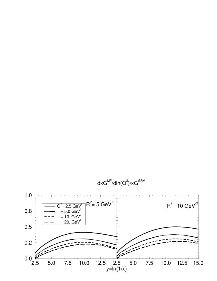
Figure 18: The average anomalous dimension for small SC (Eq. (45)).

3 First corrections to the Glauber-Mueller Approach.

In this section we discuss the corrections to the Glauber approach (the Mueller formula of Eq. (17). To understand how big could be the corrections to the Glauber approach we calculate the second iteration of the Mueller formula of Eq. (17). As has been discussed, Eq. (17) describes the rescattering of the fastest gluon ( gluon - gluon pair ) during the passage through a nucleon. In the second iteration we take into account also the rescattering of the next to the fastest gluon. This is a well defined task due to the strong ordering in the parton fractions of energy in the parton cascade in leading $ln(1/x)$ approximation of pQCD that we are dealing with. Namely

$$x_{B}\,\,<\,\,x_{n}\,\,<\,\,...\,\,<x_{1}\,\,<\,\,1\,\,,$$ (46)

where 1 corresponds to the fastest parton in the cascade.

In the first iteration, we evaluate the SC inserting the gluon distribution $xG^{DGLAP}(x,Q^{2})$ into the modified Mueller’s formula, Eq. (17). For the second iteration we substitute the correction term of the first iteration

$$x\,G\,\,=\,\,xG^{1}(x,Q^{2})({Eq.~{}(\ref{FINANS})})\,\,-\,\,x\,G^{DGLAP}(x,Q^{2})\,\,;$$ (47)

in Eq. (17) and add the first iteration to the result.

The substraction of $xG^{DGLAP}$ in Eq. (47) means that, doing the second iteration, we take into account only two or more interactions of the next to the fastest gluon with the target nucleon. We have to do such a substraction to avoid double counting since the one iteration of all gluons with the target has been included in the DGLAP evolution or in other words in the Born term of our approach ( see Ref.[11] for details).

Fig.19 shows the second iteraction calculations for our three standard observables: $R_{1}$, $<\omega>$ and $<\gamma>$. From the figure one can see that the second iteraction changes crucially the values of these parameters. As it was already noted for the nuclear case[11], a remarkable feature is the crucial change of the value of the effective power $\omega(Q^{2})$ for the “Pomeron” intercept which tends to zero at HERA kinematic region, making possible the matching with “soft” high energy phenomenology, even in the nucleon case. It is also important to note that the second iteration makes more pronounced all properties of the ratio $R_{1}$ and the anomalous dimension ( $<\gamma>$).

However, all these features of the second iteration calculations we have to consider with many restrictions. Indeed, the only conclusion which we can derive from our study is the fact that the correction to the Glauber (eikonal ) approach turns out to be large in the region of small $x$ ( $x\,<\,10^{-2}$ ) and becomes of the order of the first iteration for $x<10^{-3}$. As it has been already discussed in [5] [11], it occurs because the second iteration gives a correction of the order of $\alpha_{\rm S}ln(Q^{2}/Q_{0}^{2})ln(1/x)$, which is close to unity for the DLA of pQCD ( for the DGLAP evolution at small $x$).

Therefore, the iteration procedure cannot be an effective way to solve that problem. We have to develop a different technique to take into account rescatterings of all the partons in the parton cascade which will be more efficient than the simple iteration procedure for Eq. (17). This is the subject of the next section.

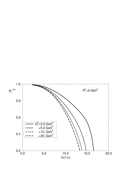
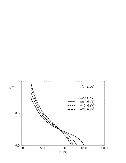
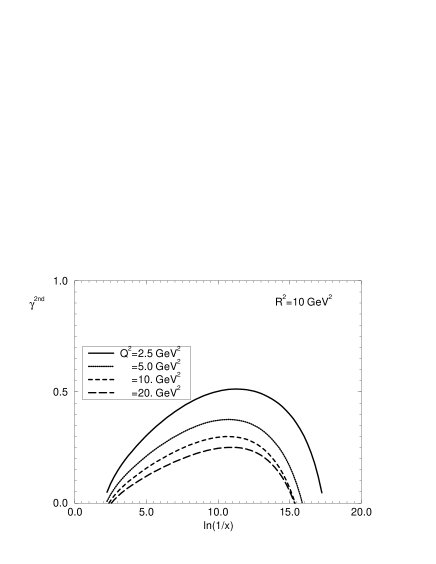
Figure 19: Second iteration calculations of $R_{1}$, $<\omega>$ and $<\gamma>$ as function of $y=ln(1/x)$ and $Q^{2}$ for two values of $R^{2}$.

4 The general approach.

4.1 Why equation?

We would like to suggest a new approach based on the new evolution equation to sum all SC. However, first of all we want to argue why an equation is better than any iteration procedure. To illustrate this point of view let us differentiate the Mueller ( see Eq. (9) ) formula with respect to $y\,=\,\ln(1/x)$ and $\xi\,=\,\ln Q^{2}$. It is easy to see that this derivative is equal to

$$\frac{\partial^{2}xG(x,Q^{2})}{\partial y\,\partial\xi}\,\,=\,\,\frac{2\,Q^{2}}{\pi^{2}}\,\int db^{2}_{t}\,\,\{\,\,1\,\,-\,\,e^{-\,\frac{1}{2}\,\sigma(x,r^{2}_{\perp}\,=\,\frac{1}{Q^{2}})\,S(b^{2}_{t})}\,\,\}\,\,.$$ (48)

A nice property of Eq. (48) is that all quantities in Eq. (48) enter at small distances, therefore it is under theoretical control. Of course, we cannot avoid all difficulties just changing the solution procedure. Indeed, the nonperturbative effects coming from the large distances are still important but they are all hidden in the boundary and initial conditions for the equation. Therefore, an equation is a good ( correct ) way to separate what we know ( small distance contribution) from that we don’t ( large distance contribution).

4.2 The generalized evolution equation.

We suggest the following way to take into account the interaction of all partons in a parton cascade with the target. Let us differentiate the $b_{t}$-integrated Mueller formula of Eq. (11) in $y\,=\,\ln(1/x)$ and $\xi=\ln(Q^{2}/Q^{2}_{0})$. It gives

$$\frac{\partial^{2}xG(y,\xi)}{\partial y\partial\xi}\,\,=\,\,\frac{2\,Q^{2}R^{2}}{\pi^{2}}\,\,\,\left\{\,\,C\,\,+\,\,ln(\kappa_{G}(x^{\prime},Q^{2}))\,\,+\,\,E_{1}(\kappa_{G}(x^{\prime},Q^{2}))\right\}\,\,\,,$$ (49)

where $\kappa_{G}(x,Q^{2})$ is given by

$$\kappa^{DGLAP}(x,Q^{2})\,\,=\,\,\frac{N_{c}\alpha_{\rm S}\pi}{2Q^{2}R^{2}}\,xG^{DGLAP}(x,Q^{2})\,\,.$$ (50)

The expression (49) can be rewritten in the form ( for fixed $\alpha_{\rm S}$ )

$$\frac{\partial^{2}\kappa_{G}(y,\xi)}{\partial y\partial\xi}\,\,+\,\,\frac{\partial\kappa_{G}(y,\xi)}{\partial y}\,\,=\,\,\frac{N_{c}\,\alpha_{\rm S}}{\pi}\,\,\left\{\,\,C\,\,+\,\,ln(\kappa_{G})\,\,+\,\,E_{1}(\kappa_{G})\right\}\,\,\equiv\,\,F(\kappa_{G})\,\,.$$ (51)

Now, let us consider the expression of Eq. (51) as an equation for $\kappa_{G}$. This equation has the following nice properties:

1. It sums all contributions of the order $(\,\alpha_{\rm S}\,y\,\xi\,)^{n}$ absorbing them in $xG(y,\xi)$, as well as all contributions of the order of $\kappa^{n}$. Therefore, this equation solves the old problem, formulated in Ref.[5], and for $N_{c}\,\rightarrow\,\infty$ Eq. (51) gives the complete solution to our problem, summing all SC;

2 .The solution of this equation matches with the solution of the DGLAP evolution equation in the DLA of perturbative QCD at $\kappa\,\rightarrow\,0$;

3. At small values of $\kappa$ ( $\kappa\,<\,1$ ) Eq. (51) gives the GLR equation. Indeed, for small $\kappa$ we can expand the r.h.s of Eq. (49) keeping only the second term. Rewriting the equation through the gluon structure function we have

$$\frac{\partial^{2}xG(y,\xi)}{\partial y\partial\xi}\,\,=\,\,\frac{\alpha_{\rm S}N_{c}}{\pi}\,xG(x,Q^{2})\,\,-\,\,\frac{\alpha_{\rm S}^{2}\,N^{2}_{c}}{8\,Q^{2}\,R^{2}}\,(xG(x,Q^{2}))^{2}\,\,,$$ (52)

which is the GLR equation [5] with the coefficient in front of the second term calculated by Mueller and Qiu [7].

4. For $\alpha_{\rm S}y\xi\,\approx\,1$ this equation gives the Glauber ( Mueller ) formula, that we have discussed in detail.

Therefore, the great advantage of this equation in comparison with the GLR one is the fact that it describes the region of large $\kappa$ and provides the correct matching both with the GLR equation and with the Glauber ( Mueller ) formula.

We propose also an equation for the $b_{t}$-dependent gluon distribution. Let us consider the $b_{t}$-dependent Mueller formula Eq. (31). Differentiating this expression in $y\,=\,\ln(1/x)$ and $\xi=\ln(Q^{2}/Q^{2}_{0})$ we obtain

$$\frac{\partial^{2}xG(y,\xi,b_{t})}{\partial y\partial\xi}\,\,=\,\,\frac{2\,Q^{2}}{\pi^{3}}\,\,\{\,\,1\,\,-\,\,e^{-\kappa_{G}(x,Q^{2},b_{t})}\,\,\}\,\,,$$ (53)

where $\kappa_{G}(x,Q^{2},b_{t})$ is given by

$$\kappa_{G}^{DGLAP}(x,Q^{2},b_{t})\,\,=\,\,\frac{N_{c}\alpha_{\rm S}\pi^{2}}{2Q^{2}}\,xG^{DGLAP}(x,Q^{2},b_{t})\,\,.$$ (54)

As it was discussed before, expression (53) can be rewritten in the form (for fixed $\alpha_{\rm S}$)

$$\frac{\partial^{2}\kappa_{G}(y,\xi,b_{t})}{\partial y\partial\xi}\,\,+\,\,\frac{\partial\kappa_{G}(y,\xi,b_{t})}{\partial y}\,\,=\,\,\frac{N_{c}\,\alpha_{\rm S}}{\pi}\,\,\,\{\,\,1\,\,-\,\,e^{-\kappa^{DGLAP}_{G}(x,Q^{2},b_{t})}\,\,\}\,\,\equiv\,\,F_{b}(\kappa_{G}^{DGLAP})\,\,.$$ (55)

Now, let us consider the expression (55) as the equation for $\kappa_{G}$. It means that we propose the following equation

$$\frac{\partial^{2}\kappa_{G}(y,\xi,b_{t})}{\partial y\partial\xi}\,\,+\,\,\frac{\partial\kappa_{G}(y,\xi,b_{t})}{\partial y}\,\,=\,\,\frac{N_{c}\,\alpha_{\rm S}}{\pi}\,\,\,\{\,\,1\,\,-\,\,e^{-\kappa_{G}(x,Q^{2},b_{t})}\,\,\}\,\,\equiv\,\,F_{b}(\kappa_{G}(x,Q^{2},b_{t}))\,\,.$$ (56)

This expression is an equation for $\kappa(y,\xi,b_{t})$. The $b_{t}$-dependent gluon distribution can be obtained from the solution of the above equation using the expression (54).

We claim that Eq. (51) and Eq. (56) solve the problem of summing all Feynman diagrams in the following kinematic region:

$$\alpha_{\rm S}\,\ln(1/x)\,\ln(Q^{2}/Q^{2}_{0})\,\,\approx\,\,1\,,$$ (57)

$$\alpha_{\rm S}\,\ln(1/x)\,\,<\,\,1\,\,,\,\,\,\,\,\,\,\,\,\,\alpha_{\rm S}\,\ln(Q^{2}/Q^{2}_{0})\,\,<\,\,1\,\,,\,\,\,\,\,\,\,\,\,\,\alpha_{\rm S}\,\,\ll\,\,1,$$ (58)

$$\alpha_{\rm S}\,\kappa\,\,\leq\,\,1\,\,.$$ (59)

The first two equations specify that we are doing our calculations in the double log approximation of pQCD while the third one introduces the new parameter $\kappa$ (see Ref.[5]) which takes into account the parton-parton interaction inside of the perturbative cascade. To illustrate how this set of parameters works let us consider an example simpler than the deep inelastic scattering with the proton, namely, the deep inelastic scattering with the meson built with heavy quarks (onia) [30]. The mass of heavy quarks ($m_{Q}$) sets the scale for the distance in this interaction, and we have $r_{\perp}\,\,\propto\,\frac{1}{m_{Q}\,\alpha_{\rm S}(m^{2}_{Q})}$. Therefore, we can safely apply pQCD for this problem.

At order $\alpha_{\rm S}^{4}(m^{2}_{Q})$ of pQCD, using the set of parameters mentioned above, the DIS can be described by the diagrams in Fig.20a. The first diagram corresponds to the DGLAP evolution equations while the second one is the Glauber - Mueller rescattering in the Born approximation. Going to the next order of pQCD, one can see that the emission of one extra gluon can be reduced: (i) to the next order correction of the DGLAP evolution equations (Fig.20b); (ii) to the emission of the extra gluon with the rapidity close to the photon and its interaction with the target ( see Fig.20c ) which has been taken into account in the generalized Eq. (51) and (ii) the emission of the extra gluon with the rapidity close to the target one ( see Fig.21a). The last one is the first from the more general class pictured in Fig.21b ( so called enhanced diagrams) that has not been included in Eq. (51). However, in Ref.[5] it has been shown that integration over $k^{2}$ as well as over rapidity $y^{\prime}$ ( see Fig.21b ) concentrated at $y^{\prime}$ close to the target rapidity and they give a small contribution of the order $\alpha_{\rm S}$ in comparison with the diagrams shown in Fig.20. Therefore, we can neglected such contribution. However, there is a danger in such an assumption, because it was made relying on perturbative estimates while Eq. (51) is a nonperturbative one. Nevertheless, the enhanced diagrams reveal themselves a class of diagrams with quite a different topology which should be discussed and calculated separately. We are going to do this job in our further publications. We must admit that only such study will be able to establish the real kinematic region where we can trust Eq. (51).

Figure 20: Diagrams of the deep inelastic scatering with heavy quarks (onia) in the order $\alpha_{\rm S}^{4}(m^{2}_{Q})$ (a) and $\alpha_{\rm S}^{5}(m^{2}_{Q})$ (b - d) of pQCD.

Figure 21: The enhanced diagrams of the deep inelastic scatering with heavy quarks (onia) (not included in Eq. (51)).

Eq. (51) is the second order differential equation in partial derivatives and we need two initial ( boundary ) conditions to specify the solution. The first one is, at fixed $y$ and $Q^{2}\,\rightarrow\,\infty$,

$$\kappa\,\,\rightarrow\,\,\frac{N_{c}\,\alpha_{\rm S}\,\pi\,}{2\,Q^{2}\,R^{2}}\,xG^{DGLAP}(x,Q^{2})\,\,.$$

The second one we can fix in the following way: at $x=x_{0}\,\,(y=y_{0})$ which is small, namely, in the kinematic region where $\alpha_{\rm S}y\xi\,\leq\,1$

$$\kappa\,\,\rightarrow\,\,\kappa_{in}\,\,=\,\,\frac{N_{c}\,\alpha_{\rm S}\,\pi}{2\,Q^{2}\,R^{2}}\,xG(x,Q^{2})\,\,,$$ (60)

where $xG$ is given by the modified Mueller formula ( see Eq. (17)). Practically, we can take $x_{0}\,=\,10^{-2}$, since the corrections to the MF are small at this value of $x=x_{0}$. However, as we have discussed, we cannot believe in any treatment of the SC at large distances. Therefore, we will take $Q_{0}^{2}\,=\,1GeV^{2}$ as the initial value of $Q^{2}$ in the modified Mueller formula. Thus, the boundary condition (60) will be considered only for $Q^{2}\,\geq\,Q^{2}_{0}\,=\,1\,GeV^{2}$. For $Q^{2}\,<\,Q^{2}_{0}$ we have to specify the initial conditions and we will discuss this point later.

The boundary condition for the $b_{t}$-dependent equation (56) is fixed in a similar form, namely, we suggest the following initial condition for $Q^{2}\,\geq Q^{2}_{0}$ where the value of $\kappa$ at $x=x_{0}$ calculated from the $b_{t}$ dependent gluon distribution

$$\kappa\,\,\rightarrow\,\,\kappa_{in}\,\,=\,\,\frac{N_{c}\,\alpha_{\rm S}\,\pi^{2}}{2\,Q^{2}}\,xG(x,Q^{2},b_{t})\,\,.$$ (61)

4.3 The asymptotic solution.

First observation is the fact that Eq. (51) has a solution which depends only on $y$. Indeed, one can check that $\kappa\,=\,\kappa_{asymp}(y)$ is the solution of the following equation

$$\frac{d\kappa_{asymp}}{dy}\,\,=\,\,F(\,\kappa_{asymp}\,)\,\,.$$ (62)

The solution to the above equation is

$$\int^{\kappa_{asymp}(y)}_{\kappa_{asymp}(y=y_{0})}\,\,\frac{d\kappa^{\prime}}{F(\kappa^{\prime})}\,\,=\,\,y-y_{0}\,\,.$$ (63)

It is easy to find the behavior of the solution to Eq. (63) at large value of $y$ since $F(\kappa)\,\,\rightarrow\,\,\bar{\alpha}_{\rm S}\ln\kappa$ at large $\kappa$ ( $\bar{\alpha}_{\rm S}=\frac{N_{c}}{\pi}\,\alpha_{\rm S}$ ). It gives

$$\kappa_{asymp}\,\,\rightarrow\,\,\bar{\alpha}_{\rm S}y\,\ln(\bar{\alpha}_{\rm S}y)\,\,\,\,\,\,at\,\,\,\,\,\,\,\bar{\alpha}_{\rm S}y\,\,\gg\,\,1\,\,.$$ (64)

At small value of $y$, $F(\kappa)\,\,\rightarrow\,\,\bar{\alpha}_{\rm S}\kappa$ and we have

$$\kappa_{asymp}\,\,\rightarrow\,\,\kappa_{asymp}(y=y_{0})\,\,e^{\bar{\alpha}_{\rm S}(y-y_{0})}\,\,.$$ (65)

We claim this solution is the asymptotic solution to Eq. (51). To prove this we have to consider the stability of the asymptotic solution. It means, that we solve our general equation looking for the solution in the form

$$\kappa\,\,=\,\,\kappa_{asymp}(y)\,\,+\,\,\Delta\kappa(y,\xi-\xi_{0})\,\,,$$ (66)

where $\Delta\kappa$ is small ($\Delta\kappa\,\ll\,\kappa_{asymp}$) but an arbitrary function at $\xi\,=\,\xi_{0}$. We have to prove that Eq. (51) will not lead to big $\Delta\kappa$ ($\Delta\kappa\,\gg\,\kappa_{asymp}$) at large $\xi$.

The following linear equation can be written for $\Delta\kappa$

$$\frac{\partial^{2}\Delta\kappa(y,\xi)}{\partial y\,\partial\xi}\,\,+\,\,\frac{\partial\Delta\kappa(y,\xi)}{\partial y}\,\,=\,\,\frac{dF(\kappa)}{d\kappa}\,|_{\kappa=\kappa_{asymp}(y)}\,\,\Delta\kappa(y,\xi)\,\,.$$ (67)

In Ref.[11] was proven, that the solution of Eq. (67) is much smaller than $\kappa$, since $\frac{dF(\kappa)}{d\kappa}\,\,\rightarrow\,\,0$ at large $y$.

The $b_{t}$-dependent equation also has an asymptotic solution. Indeed, one can check that $\kappa\,=\,\kappa_{asymp}(y,b_{t})$ is the solution of the following equation

$$\frac{d\kappa_{asymp}}{dy}\,\,=\,\,F_{b_{t}}(\,\kappa_{asymp}\,)\,\,,$$ (68)

which can be rewritten as

$$\int^{\kappa_{asymp}(y,b_{t})}_{\kappa_{asymp}(y=y_{0},b_{t})}\,\,\frac{d\kappa^{\prime}}{F_{b_{t}}(\kappa^{\prime})}\,\,=\,\,y-y_{0}\,\,.$$ (69)

This equation has the solution

$$\kappa_{asymp}(y,b_{t})\,\,=\,\,\ln\{1\,\,+\,\,(\,e^{\kappa_{0}(y=y_{0},b_{t})}\,\,-\,\,1\,)\,e^{\frac{N_{c}\alpha_{\rm S}}{\pi}\,(y\,-\,y_{0})}\,\}\,\,.$$ (70)

It is easy to find from Eq. (70) the behavior of the solution of Eq. (68) at large values of $y$. It gives

$$\kappa_{asymp}(y;b_{t})\,\,\rightarrow\,\,\bar{\alpha}_{\rm S}y\,\,\,\,\,\,\mbox{at}\,\,\,\,\,\,\,\bar{\alpha}_{\rm S}y\,\,\gg\,\,1\,\,.$$ (71)

At small values of $y$, we have

$$\kappa_{asymp}(y,b_{t})\,\,\rightarrow\,\,\kappa_{asymp}(y=y_{0},b_{t})\,\,e^{\bar{\alpha}_{\rm S}(y-y_{0})}\,\,.$$ (72)

Therefore, the asymptotic solution has a chance to be the solution of equation (51) ((56) for $b_{t}$-dependent case) in the region of very small $x$. To prove that, we need to solve the equation in the wide kinematic region starting with the initial condition. We managed to do this only in the semiclassical approach.

4.4 The semiclassical approach.

In the semiclassical approach the solution of eq. (51) is supposed to be in the form

$$\kappa=e^{S}\,,$$ (73)

where $S$ is a function with partial derivatives: $\frac{\partial S}{\partial y}=\omega$ and $\frac{\partial S}{\partial\xi}=\gamma$ which are smooth functions of $y$ and $\xi$. It means that

$$\frac{\partial^{2}S}{\partial\xi\partial y}\ll\frac{\partial S}{\partial y}\frac{\partial S}{\partial\xi}=\omega\gamma\,\,.$$ (74)

Using eq.(74), one can rewrite eq.(51) in the form

$$\frac{\partial S}{\partial y}\frac{\partial S}{\partial\xi}+\frac{\partial S}{\partial y}=e^{-S}F(e^{S})\equiv\Phi(S)$$ (75)

or

$$\omega(\gamma+1)=\Phi(S)\,\,.$$ (76)

For an equation in the form

$$F(\xi,y,S,\gamma,\omega)=0\,,$$ (77)

we can introduce the set of characteristic lines $(\xi(y),S(y),\omega(y),\gamma(y))$, which satisfy a set of well defined equations (see, for example, Refs. [31], [32] for the method). In Ref. [11] we developed a detailed calculation of the solution. Here, we will concentrate on the $b_{t}$ dependent evolution. To solve the $b_{t}$ dependent equation in the semiclassical approach, we need only to substitute the nonlinear term $F_{b_{t}}(\kappa)$, instead of $F(\kappa)$, in the expression (75). Using eq.(75) and eq.(76), written for $\Phi_{b_{t}}$, we obtain the following set of equations for the characteristics

$$\frac{d\xi}{dy}=\frac{\Phi_{b_{t}}(S)}{(\gamma+1)^{2}}\,;\,\,\,\,\,\frac{dS}{dy}=\frac{2\gamma+1}{(\gamma+1)^{2}}\Phi_{b_{t}}(S)\,;\,\,\,\,\frac{d\gamma}{dy}=\Phi^{\prime}_{S;b_{t}}\frac{\gamma}{\gamma+1}\,\,,$$ (78)

where $\Phi^{\prime}_{S;b_{t}}\,=\,\frac{\partial\Phi_{b_{t}}}{\partial S}$. The initial conditions for this set of equations we derive from eq.(60), being

$$S_{0} = ln\kappa_{in}(y_{0},\xi_{0})\,,$$

$$\gamma_{0} = \left.\frac{\partial ln\kappa_{in}(y_{0},\xi)}{\partial\xi}\right|_{\xi=\xi_{0}}\,.$$ (79)

The DGLAP equation for $\kappa$ is obtained taking the term in the curly in r.h.s of Eq. (51) equal to $\kappa$, which gives $\Phi=\frac{\alpha_{\rm S}Nc}{\pi}$ and $\Phi^{\prime}_{S,b_{t}}\,=\,0$ in Eq. (78). The main properties of these equations have been considered in Ref.[11] analytically. Here, however, we restrict ourselves mostly to the numeric solution of these equations.

For $Q^{2}\,\leq\,Q^{2}_{0}$ we cannot specify the initial condition. To find characteristics which correspond to such small virtualities, we put a boundary condition at $Q^{2}=Q^{2}_{0}$, namely $\kappa_{bound}\,=\,\kappa(y,\xi=\xi_{0})$. However, this boundary condition cannot be arbitrary at $x\,\rightarrow\,0$, but it should satisfy the equation. On the other hand we wish to incorporate in this boundary condition everything that has been known on the parton densities experimentally. We suggest the following boundary condition:

$$\kappa_{bound}\,\,=\,\,\kappa^{GRV}(Q^{2}=Q^{2}_{0},x;b_{t})\,\,\,\,\,at\,\,\,\,x\,\geq\,x_{0}\,\,;$$ (80)

$$\kappa_{bound}\,\,=\,\,\kappa_{asymp}\,\,\,\,\,at\,\,\,\,x\,\leq\,x_{0}\,\,,$$

where the value of $x_{0}$ we find from the equation

$$\kappa^{GRV}(Q^{2}=Q^{2}_{0},x=x_{0};b_{t})\,\,=\,\,1\,\,.$$

Using Eq. (80) we can specify the boundary condition for our set of equations, namely

$$S_{0}(\xi=\xi_{0},b_{t})\,\,=\,\,\ln(\kappa_{bound}(y_{0},\xi_{0};b_{t})\,\,;$$ (81)

$$\omega_{0}(\xi=\xi_{0})\,\,=\,\,\frac{\partial\ln(\kappa_{bound}(\xi_{0},y;b_{t})}{\partial y}|_{y=y_{0}}\,\,.$$

Using the boundary conditions of Eq. (81), it is better to rewrite Eq. (78) in the form:

$$\frac{d\xi}{dy}\,\,=\,\,\frac{\omega^{2}}{\Phi_{b_{t}}(S)}\,\,;\,\,\,\,\frac{dS}{dy}\,\,=\,\,2\,\omega\,+\,\frac{\omega^{2}}{\Phi_{b_{t}}(S)}\,\,;\,\,\,\,\frac{d\omega}{dy}\,\,=\,\,\omega^{2}\,\frac{\Phi^{\prime}_{S;b_{t}}(S)}{\Phi_{b_{t}}(S)}\,\,.$$ (82)

We would like to emphasize that our suggestion ( see Eq. (80) ) is still rather arbitrary since the equation for $x_{0}$ has no deep theoretical arguments. Actually, what we know theoretically is the fact that $\kappa_{bound}\,\rightarrow\,\kappa_{asymp}$ at $\kappa^{GRV}\,\geq\,1$. This is the reason why we decided to restrict ourselves to the solution of the equation for the trajectories that started at $y=5$ with the values of $Q^{2}\,\geq\,Q^{2}_{0}\,=\,1\,GeV^{2}$. We are studing other trajectories on a separate paper.

For the numerical solution we use the 4th order Runge - Kutta method to solve our set of equations with the initial distributions of Eq. (79). For a short notation we will use AGL to our nonlinear evolution equation Eq. (51) and AGL${}_{b_{t}}$ for the $b_{t}$ dependent nonlinear evolution equation Eq. (56). Fig.22 shows the general features of the solution. Fig.22a shows the characteristic curves in the $y$ v.s. $\xi$ plane for different initial conditions. Fig.22b shows the evolution of the respective $\gamma$ values with $y$. The initial conditions, plotted in Fig.(23), are calculated for $y=4.6$ ($x\,\approx\,10^{-2}$) and $Q^{2}_{0}$ from $1\,GeV^{2}$ to $3.4\,GeV^{2}$ with $R^{2}\,=\,5\,GeV^{-2}$. When $\gamma$ goes to zero as $y$ grows, the nonlinear effects play an important role. The respective trajectory tends to a vertical line, and the AGL solution tends to the asymptotic one. When $\gamma$ goes to a constant, the AGL solution tends to the DGLAP one.

Figure 22: The trajectories (a) and the $\gamma$ values (b) for the solution of the generalized evolution equation for nucleon with $R^{2}=\,5\,GeV^{-2}$.

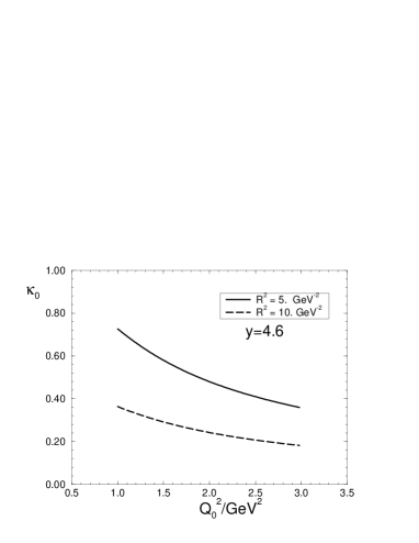
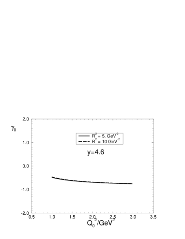
Figure 23: The initial values $\kappa_{0}$ and $\gamma_{0}$ for $y=4.6$ as a function of $Q^{2}_{0}$.

4.5 Comparison between different approaches to the SC

Using the characteristics and the initial conditions we are able to find the solution of AGL equation as a function of $y$ and $\xi$. For a given point $(\,y_{1},\,\xi_{1}\,)$, we vary the initial condition until we find the characteristic which passes throught the point. From the characteristic we can reconstruct the solution. The same procedure can be used for GLR equation. In Fig.24 we compare the $\kappa$ values obtained from the solution of the nonlinear equation (51) (AGL) and the GLR equation. The values of $\kappa$ calculated from the modified Mueller Formula ( MOD MF) and from the DGLAP evolution equation (GRV distribution) are also shown. The results are presented as functions of $y$ for several values of $Q^{2}$. The initial condition is the same for all equations.

Figure 24: The $\kappa$ values solutions of the nonlinear equation (AGL) and the GLR equation. The values of $\kappa$ calculated from the modified Mueller Formula for the gluon distribution (MF) and from the DGLAP gluon distribution is also shown.

We can see from Fig.24 that the SC predicted by the MOD MF, the AGL equation and by GLR equation have the same order of magnitude at HERA kinematic region ($5\,<\,y\,<10$). For very small $x$ ($y\,>\,10$) the results are quite different. The values of $\kappa$ obtained from the AGL equation suffer a sizeable reduction when compared with those obtained from the modified Mueller formula. The AGL solution increases monotonically with $y$, but much less then the Mueller formula. The GLR equation gives much stronger SC. In fact, the GLR equation predicts saturation at very small $x$ values.

In Fig.25, we present the solution of the AGL equation compared with the AGL_asymp results. For each value of $Q^{2}$, the asymptotic equation is solved backwards from the value of $\kappa$, solution of AGL equation (we took $y\,=\,29.1$). We can see from the figure that the asymptotic solution crosses the AGL solution twice for $Q^{2}\,\leq\,5\,GeV^{2}$. We suppose it occurs because the AGL solution have not yet reached its asymptotic value for that $y$.

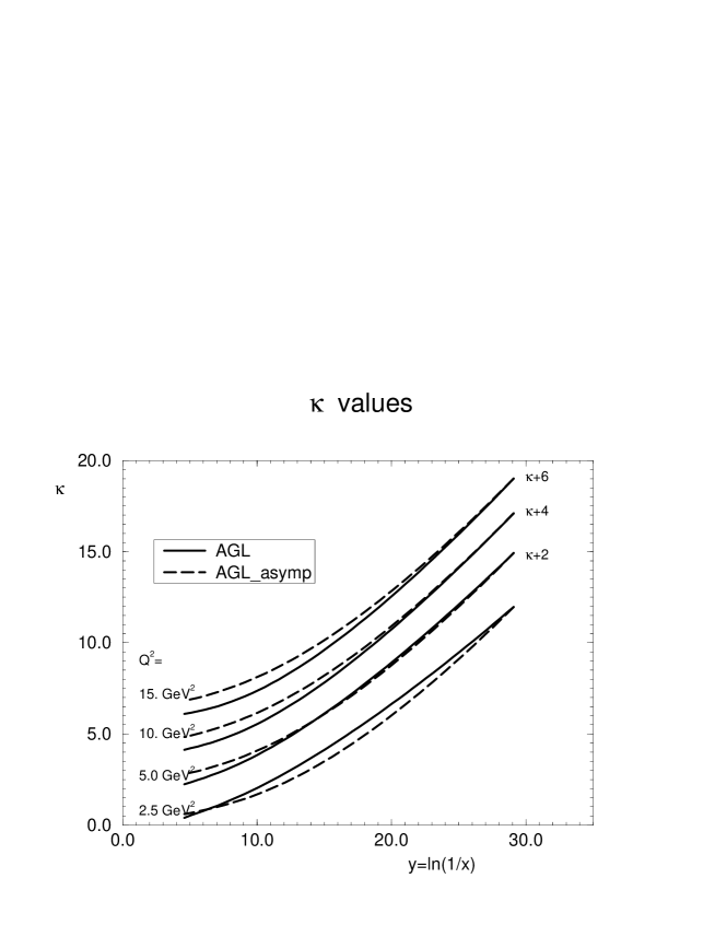
Figure 25: The $\kappa$ values solutions of the nonlinear equation (AGL) compared with the backwards evolution of the asymptotic equation.

We would like to draw your attention to the fact that our asymptotic solution turns out to be quite different from the GLR one. The GLR solution in the region of very small $x$ leads to saturation of the gluon density [31, 32, 33]. Saturation means that $\kappa$ tends to a constant in the region of small $x$. The solutions of Eq. (51) approach the asymptotic solution at $x\,\rightarrow\,0$, which does not depend on $Q^{2}$, but exhibits sufficiently strong dependence of $\kappa$ on $x$ ( see Fig.25 ), namely $\kappa\,\propto\,\alpha_{\rm S}\ln(1/x)\ln\ln(1/x)$. The absence of saturation does not contradict any physics since gluons are bosons and it is possible to have a lot of bosons in the same cell of the phase space. We should admit that A. Mueller first came to the same conclusion using his formula in Ref.[10].

To complete our discussion, we present in Fig.26 the solutions of the $b_{t}$-dependent nonlinear equation (AGL${}_{b_{t}}$) calculated at $b_{t}^{2}=0$ for different values for $Q^{2}$ and $R^{2}=5\,GeV^{-2}$. One can see that the scale of the SC is much bigger for $b_{t}$ =0 than for integrated over $b_{t}$ case. The solutions approach the straight line behaviour for $y$ close to its initial value. It occurs because the AGL${}_{b_{t}}$ equation reaches its asymptotic behaviour for $\kappa(b_{t})$ close to the initial condition. Therefore, we can use the asymptotic solution as a good approximation to the general solution of the equation at small values of $b_{t}$.

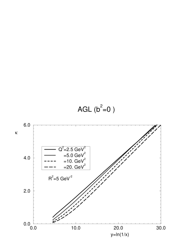
Figure 26: The $\kappa$ values solutions of the $b_{t}$-dependent nonlinear equation (AGL${}_{b_{t}}$) calculated for $b_{t}^{2}=0$.

4.6 The $F_{2}$ structure function from the general approach.

In order to obtain the $F_{2}$ structure function from the general approach, we calculate the valence and charm components of $F_{2}$ as described in the section 2.5. We suppose that the sea component is generated mainly from the scale violation mechanism. Thus, the sea component of $F_{2}$ can be calculated by the simplified formula

$$F_{2}^{SEA}(x,Q^{2}) = F_{2}(x,Q^{2}_{0})\,+\,\frac{1}{2\pi}\sum^{N_{f}}_{1}\,\,Z^{2}_{f}\,\int^{\ln Q^{2}}_{\ln Q^{2}_{0}}\alpha_{\rm S}(Q^{\prime 2},N_{f})d(\ln Q^{\prime 2})$$ (83)

$$\int^{1-x}_{0}\,dz\,\,[z^{2}+(1-z)^{2}]\{\frac{x}{1-z}G(\frac{x}{1-z},Q^{\prime 2})\}\,\,,$$

where $F_{2}(x,Q^{2}_{0})$ is the value of the sea component of $F_{2}$ at $Q^{2}=Q_{0}^{2}$. In this approach, we include the SC in the gluon distribution in the expression (83). In Fig.27 we show the results of $F_{2}$ with the sea component calculated from different gluon distributions using expression (83) for the sea component. The valence, charm, and the initial value of the sea component (at $Q^{2}\,=\,Q_{0}^{2}=1\,GeV^{2}$) are calculated from the GRV distributions. We can see from the figure that the SC predicted by the AGL and GLR equations are negligible for $y\,<\,7$. For $y\,>\,7$, the SC start to become important. This result can be understood if we look at Fig.24. The $\kappa$ values given by the DGLAP, AGL and GLR equations are very close for $Q^{2}<10\,GeV^{2}$ and $y\,<\,7$, i.e., negligible SC are predicted in this region. The results presented in Fig.27 are consistent with that presented in Fig.11.

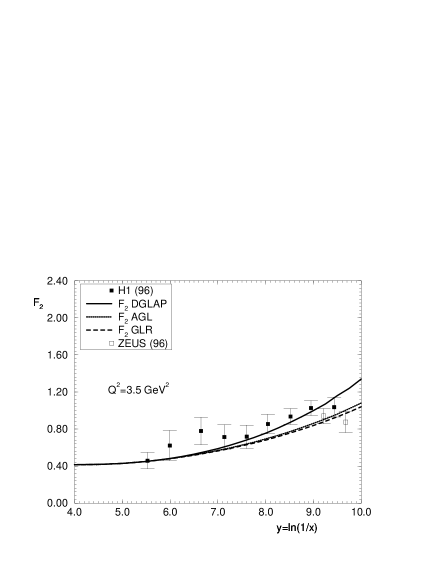
Figure 27: $F_{2}$ calculated from different gluon distributions using the expression (83) for the sea component.

5 Conclusions.

In this paper we re-analyse the situation of the shadowing corrections in QCD for proton deep inelastic structure functions. As have been discussed in the introduction we view the physical interpretation of HERA data as controversial. Here, we are going to summarize the result of our analysis of the value of the SC, listing the questions that we asked ourselves and the answers we got in the paper.

1. Can we provide reliable estimates for the value of the SC in QCD?

Our answer is yes and, to answer this question, we reconsidered the Glauber - Mueller approach for the SC in DIS [10] and suggested the modified Mueller formula ( see Eq. (17)) to estimate the scale of the SC. We consider these estimates as estimates from below for two reasons: (i) in the eikonal (Glauber - Mueller ) approach only the fastest partons interact with the target and, therefore, the real value of the SC should be bigger; (ii) we cannot trust the pQCD approach at large distances which enter into our formulae, in spite of the fact that the Mueller formula gives the infrared stable answer for the deep inelastic structure functions. We introduce a scale $r^{2}_{0}\,=\,\frac{1}{Q^{2}_{0}}$ and calculate only the SC from the distances $r_{\perp}\,\leq\,r_{0}$. We chose $Q_{0}=1\,GeV$, relying on the fact, that all available parameterizations of the deep inelastic structure functions describes the data down to photon virtuality $Q^{2}=Q^{2}_{0}=1\,\,GeV^{2}$. We checked that the modified Mueller formula gives the small corrections to $F_{2}(x,Q^{2})$ at large values of $Q^{2}$ as well as to the momentum sum rules. We believe that we are able to give a reliable estimate of the minimal value of the possible SC to the parton densities.

2. What is the value of the SC?

Using the modified Mueller formula we obtained the estimates for the value of the SC given in Figs.(5), (6) and (7). These figures show that the SC are essential in HERA kinematic region to gluon densities, especially to $<\gamma>$ and $<\omega>$. We calculated also the SC for $b_{t}$ distributions and showed that the SC at $b_{t}=0$ turn out to be much bigger than the integrated over the $b_{t}$ parton densities. One can see from Figs.(12) that $<\gamma(b_{t}=0)>$ is smaller that $\gamma=\frac{1}{2}$ for $Q^{2}$ smaller then $10\,GeV^{2}$ and $<\omega(b_{t}=0)>$ reaches the value of the intercept of the soft Pomeron making possible the matching of soft and hard processes. Therefore, our answer to the question formulated in the title of this subsection is that the value of the SC is big enough to be seen in the gluon structure function at HERA kinematic region. However, the SC to $F_{2}(x,Q^{2})$ turns out to be rather small. This is a reason why the SC has not been observed and the whole issue of the SC has been hidden in uncertainties of the value of the gluon structure function in current attempts to describe the HERA data in the framework of the DGLAP evolution.

We would like to point out that all numbers were calculated using the GRV parameterization for the gluon structure function and our reasoning for the choice of the GRV parameterization is (i) it describes the experimental data for $Q^{2}\geq 1GeV^{2}$; (ii) the initial virtuality in the GRV parametrization is very low ( $Q^{2}_{0}=0.3GeV^{2}$) and, therefore, the DLA of pQCD works better than in the other parameterizations ( we recall that the Mueller formula for the SC was proven in the DLA). However, we are planning to calculate the value of the SC using other parameterization in future. It remains also for further publications the important question how the value of the SC depends on the choice of the initial parton distribution at fixed value of $x$.

3. Where is the BFKL Pomeron?

Our answer is that the BFKL Pomeron is hidden under the SC. We argue this point in subsection 2.9. Here, we want to repeat that this statement depends crucially on the choice of the gluon correlation radius $R^{2}$ and we argued that HERA data gives $R^{2}=5\,GeV^{-2}$. This result means that the break of the operator product expansion appears rather as the result of the SC than the BFKL dynamics ( see Ref.[22] ). We also argued that the BFKL Pomeron should not be seen in all other processes even in the inclusive production of the jet in DIS which was specially proposed to test the BFKL Pomeron[24], since for all these processes $R^{2}$ is smaller than for the proton target. We have to search for new processes to recover the BFKL dynamics. It is interesting to notice that the fact that the BFKL Pomeron is hidden under the SC is seen directly from Figs.1 and 2 by comparing two curves: $\kappa\,=\,1$ and $<\gamma>\,=\,\frac{1}{2}$. One can notice that the first curve is to the right of the second one. It means that decreasing the value of $Q^{2}$ at any fixed $x$ we meet first the curve $\kappa\,=\,1$ where the SC become essential and only for smaller value of $Q^{2}$ we approach the curve $<\gamma>\,=\,\frac{1}{2}$ where the BFKL dynamics could enter in the game.

4. How well works the Glauber - Mueller approach?

We showed that the corrections to the Glauber - Mueller approach are big and it can give only estimates from below for the value of the SC ( see section 3 ).

5. Can we develop a general approach in QCD to calculate the SC?

Our answer is that we can. We suggest the new evolution equation and discussed its theoretical accuracy. We argued that this equation solves the problem of the SC summing up all diagrams of the order $(\alpha_{\rm S}\ln(1/x)\ln(Q^{2}/Q^{2}_{0}))^{n}$ and $(\kappa)^{n}$ considering $\alpha_{\rm S}\ln(1/x)\ll 1$, $\alpha_{\rm S}\ln(Q^{2}/Q^{2}_{0})\ll 1$, $\alpha_{\rm S}\ll 1$ and $\kappa\ll 1$, where $\kappa=\frac{3\pi\alpha_{\rm S}}{2\,Q^{2}R^{2}}xG(x,Q^{2})$. This equation allows us to calculate the value of the SC in a wider kinematic region than the GLR equation and study the parton density to the left of the critical line of the GLR equation ( $<\gamma>=1/2$).

6. Do the parton densities reach saturation?

Our answer is no. We solve the new evolution equation and found out that the gluon density $xG(x,Q^{2})$ tends to the asymptotic behaviour ( $xG(x,Q^{2})\,\rightarrow xG^{asym}(x,Q^{2})=2R^{2}Q^{2}\ln(1/x)\ln\ln(1/x)$). We discuss the more detailed comparison of the solution to the new evolution equation with the GLR one in subsection 4.3.

7. Can we match the deep inelastic cross section with the cross section of the real photoproduction?

We proved that the solution of the new evolution equation gives the mild behaviour of the parton densities with energy (asymptotically, they tend to $\ln(W)$ ). It gives us a hope to describe the matching between soft and hard processes taken into account the SC using the new evolution equation. We suppose to do this in our further publications.

8. What can be a practical use of our approach?

We were impressed by the fact that HERA data on $F_{2}(x,Q^{2})$ can be fitted by the simple formula [34]:

$$F_{2}(x,Q^{2})\,\,=\,\,m\log\frac{Q^{2}}{Q^{2}_{0}}\,\log\frac{x_{0}}{x}\,\,,$$

where $m=0.377$, $x_{0}=0.074$ and $Q^{2}_{0}=0.5GeV^{2}$. Such a parameterization leads to the gluon structure function [34] $xG(x,Q^{2})\,=\,3\log(x_{0}/x)$, which energy ($x$) dependence is just the same as for the solution to our evolution equation. Therefore, we can interpret our results as the theoretical justification of the Buchmuller - Haidt parameterization. Our physical idea sounds as follows: everything has happened at $x$ of the order of $10^{-2}$, at such values of $x$ the parton densities have reached their asymptotic values and we see only asymptotic behaviour of the parton densities at smaller values of $x$. We suppose to work out this idea in the nearest future.

9. Has everything been done?

Of course, the answer is no. We have a lot of problems to solve. First, as we have mentioned, we need to estimate the values of the SC using other parameterizations of the parton densities but not only the GRV one. We have to study more carefully the dependence of the value of the SC on the initial parton distributions and to check how stable are our results. Second, we have to find the complete solution for the running $\alpha_{\rm S}$. The experience with the GLR equation shows that the running $\alpha_{\rm S}$ leads to important properties of the SC as the appearance of the critical line and so on. Third, we need to take into account that the partons in the parton cascade can interact not only with the target but with the other partons (so called enhanced diagrams). We can find out the region of the applicability of the new equation only after solving this problem. We suppose to do this as the next step in our approach.

We believe that our paper is only the first step in reconsidering the whole issue of the SC in DIS. Actually, we showed here, that the new parameter that governs the size of the SC is $\kappa$ and the value of the SC is not negligible in HERA kinematic region. This conclusion makes rather suspicious the current interpretation of HERA data on the basis of the DGLAP evolution equations without the SC and much work is needed to clarify physics of DIS that is behind HERA data.

While completing this paper, our attention was drawn to three recent papers [35] [36] [37] which deal with the Glauber - Mueller approach to the SC for the deep inelastic structure function $F_{2}(x,Q^{2})$ for nuclei and for the hard diffractive production. The results obtained in these paper are close to ours.

Acknowledgements: E. Levin wish to thank E. Gotsman and U. Maor for stimulating discussions as well as all participants of the theory seminar in HEP department of the Tel Aviv university for encouraging criticism and interest. Work partially financed by CNPq, CAPES and FINEP, Brazil.

References

-
[1]
ZEUS collaboration, M. Derrick et.al.:Zeit. Phys. C65 (1995) 379;
H1 collaboration, T. Ahmed et.al: Nucl. Phys. B439 (1995) 471;
H1 collaboration, S. Aid et al.: Nucl. Phys. B470 (1996) 3 - [2] A.D. Martin, R.G. Roberts and W.J. Stirling: Phys. Lett. B306 (1993) 145.
- [3] CTEQ Collaboration, H.L.Lai et al.: Phys. Rev. D51 (1995) 4763.
- [4] M. Gluck, E. Reya and A. Vogt: Z. Phys. C53 (1992) 127. M. Gluck, E. Reya and A. Vogt: Z. Phys. C67 (1995) 433.
- [5] L. V. Gribov, E. M. Levin and M. G. Ryskin: Phys.Rep. 100 (1983) 1.
- [6] A.L. Ayala, M.B. Gay Ducati and E.M. Levin: Phys. Lett. B388 (1996) 188
- [7] A.H. Mueller and J. Qiu: Nucl. Phys. B268 (1986) 427.
- [8] E.A. Kuraev, L.N. Lipatov and V.S. Fadin: Sov. Phys. JETP 45 (1977) 199 ; Ya.Ya. Balitskii and L.V. Lipatov:Sov. J. Nucl. Phys. 28 (1978) 822; L.N. Lipatov: Sov. Phys. JETP 63 (1986) 904.
- [9] E.M. Levin and M.G.Ryskin: Sov. J. Nucl. Phys. 45 (1987) 150.
- [10] A.H. Mueller: Nucl. Phys. B335 (1990) 115;
- [11] A.L. Ayala, M.B. Gay Ducati and E.M. Levin: CBPF-FN-020/96, hep-ph 9604383, April 1996; to appear in Nucl. Phys. B.
- [12] M.G. Ryskin: Z. Phys. C57 (1993) 89.
- [13] S. Brodsky et al: Phys. Rev. D50 (1994) 3134.
- [14] V.N. Gribov and L.N. Lipatov:Sov. J. Nucl. Phys. 15 (1972) 438; L.N. Lipatov: Yad. Fiz. 20 (1974) 181; G. Altarelli and G. Parisi:Nucl. Phys. B126 (1977) 298; Yu.L. Dokshitser:Sov. Phys. JETP 46 (1977) 641.
- [15] V.A.Abramovski, V.N. Gribov and O.V. Kancheli: Sov. J. Nucl. Phys. 18 (1973) 308.
- [16] M. Abramowitz and I.A. Stegun: “Handbook of Mathematical Functions”, Dover Publication, INC, NY 1970.
- [17] G.Veneziano: Phys. Lett. B52 (1974) 220, Nucl. Phys. B74 (1974) 365; G. Marchesini and G. Veneziano: Phys. Lett. B56 (1975) 271; M. Ciafaloni, G. Marchesini and G. Veneziano: Nucl. Phys. B98 (1975) 472.
- [18] J.Bartels: Z. Phys. C60 (1993) 471, Phys. Lett. B298 (1992) 589; E.M. Levin, M.G. Ryskin and A.G. Shuvaev: Nucl. Phys. B387 (1992) 204.
- [19] L. N. Lipatov: Hep-ph/9610276, Octorber, 1996.
- [20] T. Jaroszewicz: Phys. Lett. B116 (1982) 291.
- [21] G. Marchesini and B. Webber: Nucl. Phys. B349 (1991) 617; E.M. Levin, G. Marchesini, M.G. Ryskin and B. Webber: Nucl. Phys. B357 (1991) 167.
- [22] A.H. Mueller: Phys. Lett. B396 (1997) 251.
- [23] E.M. Levin: Nucl. Phys. B453 (1995) 303.
- [24] A.H. Mueller: Nucl. Phys. B ( Proc. Suppl.)18C(1991) 125; J. Bartels, A. DeRoeck and M. Loewe: Z. Phys. C54 (1992) 635; J. Kwiecinski, A.D. Martin, P.J. Sutton: Phys. Lett. B287 (1992) 254, Phys. Rev. D46 (1992) 921;W-K. Tang: Phys. Lett. B278 (1991) 363;J. Bartels:J. Phys.G19(1993)1611; E. Laenen and E. Levin:J. Phys.G19(1993)1582.
- [25] E. Laenen and E. Levin: Ann. Rev. Nucl. Part. 44 (1994) 199.
- [26] R.K. Ellis, Z. Kunst and E. M. Levin: Nucl. Phys. B420 (1994) 517.
- [27] J. Bartels and M.G. Ryskin: DESY - 96 - 238, hep-ph 9612226.
- [28] A. Donnachie and P.V. Landshoff: Phys. Lett. B185 (1987) 403, Nucl. Phys. B311 (1989) 509; E. Gotsman, E. Levin and U. Maor: Phys. Lett. B353 (1995) 526.
- [29] M. Gluck, E. Reya and A. Vogt: Z. Phys. C67 (1995) 433.
- [30] A.H. Mueller: Nucl. Phys. B415 (1994) 373.
- [31] J.C. Collins and J. Kwiecinski: Nucl. Phys. B335 (1990) 89.
- [32] J. Bartels, J. Blumlein and G. Shuler: Z. Phys. C50 (1991) 91.
- [33] J. Bartels. and E. Levin: Nucl. Phys. B387 (1992) 617.
- [34] W. Buchmüller and D. Haidt: Hep-ph/9605428, May, 1996.
- [35] Zheng Huang, Hung Jung Lu and Ina Sarcevic: AZPH - TH - 97 - 07, hep - ph /9705250.
- [36] E.Gotsman,E. Levin and U. Maor: TAUP 2405/97, hep - ph/9701226.
- [37] L. Frankfurt, W. Koepf and M. Strikman: OSU - 97 - 0201, hep - ph /9702216.