1. Exclusive virtual Compton scattering (VCS) has some very interesting features. The subject has a long history, being examined early in the development of the parton model [1]. Recently [2, 3, 4] there has been considerable renewed interest with the realization that off-diagonal correlations of quark operators in proton states might be measurable with VCS. They generalize the parton distributions of deep inelastic scattering (DIS) but, being off-diagonal matrix elements, do not have a probability interpretation. In fact, these “off-diagonal parton distributions” have a long history [5]. Following the work of Ji, Tang and Hoodbhoy [6], Ji pointed out the relevance of VCS to getting information about quark orbital angular momentum [2]. Some analysis in the operator product expansion has been done in  [7, 8].

In DIS the diagrams that contribute at leading twist to the cross section factorize into a hard perturbative and a soft nonperturbative part, which are connected by only two quark or two gluon legs, where furthermore the corresponding loop integral only runs over the parton momentum fraction $x$. This defines the handbag approximation. Such diagrams evidently also contribute to the VCS amplitude. We show in Fig. 1 the handbag diagrams at Born level. To higher order in $\alpha_{S}$, one has quark diagrams with radiative corrections to the hard scattering parts, as well as diagrams where the two partons attached to the soft blob are gluons.

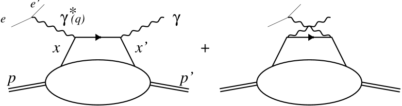
Figure 1: The handbag Born diagrams for virtual Compton scattering. Here $x$ and $x^{\prime}$ are light cone fractions of the quark with respect to the incoming proton momentum.

There is no doubt that the handbag diagrams are but a subset of those contributing to the process. Considerable theoretical effort has already gone into exploiting the properties of the handbag model, for instance, studying logarithmic scaling violations [2, 3, 8]. A much different question is to critically ask how well one can trust to the dominance of the handbag model in the first place. On the practical side, the new elements of VCS, off-diagonal in momentum and spin, with the complication of a real photon in the final state, are not dynamically similar to inclusive electroproduction but rather to other exclusive reactions. In particular the size of (higher twist) corrections to the handbag contribution, such as for instance the pion exchange process discussed in [9], really has to be studied anew empirically: the values of $Q^{2}$ where the handbag approximation is satisfactory need not be the same in deep inelastic scattering and in VCS. At this point in time, not enough is known to make iron-clad statements directly from theory. As we argue below, the scope of the handbag is most probably limited to a restricted kinematic region. But whatever theory statements are made, the function of experimental science is to test the important ideas systematically. A very diverse experimental program is now being discussed for JLAB, HERA, CERN and the ELFE project [10].

The dynamics of VCS is quite rich, and very different physical processes will occur in different kinematic regions. No single mechanism can be expected to describe all regions. Our approach here is to ask: how can one test experimentally the dominance of the general model, allowing for lack of information about the new parton distributions about which almost nothing is known so far? To proceed we will first focus on the kinematic regions where the model might work, and then find some tests based on general principles.

2. Let us then have a closer look at the kinematics of the process

$$\gamma^{\ast}(q)+p(p)\to\gamma(q^{\prime})+p(p^{\prime})\hskip 6.0pt,\hskip 6.0pt$$ (1)

with momenta given in parentheses. We use the conventional variables

$$Q^{2}=-q^{2}\hskip 6.0pt,\hskip 6.0ptW^{2}=(p+q)^{2}\hskip 6.0pt,\hskip 6.0ptx_{B}=Q^{2}/(2p\cdot q)\hskip 6.0pt,\hskip 6.0pt$$ (2)

and consider only $Q^{2}\gg 1\mbox{\ GeV}^{2}$ so that pQCD may be applied. Taking $Q^{2}$ large while keeping $x_{B}$ fixed corresponds to the “Bjorken limit”, but for our reaction is too broad a range for the handbag’s application. In fact, much of the physics hinges on the different components of the four-vector $\Delta^{\mu}=(p-p^{\prime})^{\mu}$. Note that $\Delta^{2}=t$ is the additional Mandelstam variable necessary to fix the kinematics. We will always work in the $\gamma^{\ast}p$ center of mass, with the positive $z$-axis given by the virtual photon momentum, and introduce $\Delta_{T}$ as the transverse momentum transfer from the initial proton to the final one. For the scattering angle $\theta$ between $p$ and $p^{\prime}$ we have

$$\sin\theta=\frac{2\Delta_{T}W}{W^{2}-m^{2}}\hskip 6.0pt.\hskip 6.0pt$$ (3)

At $\theta=0$ the invariant $t$ attains its kinematical limit, given by

$$t_{0}=-m^{2}\frac{x_{B}^{2}}{1-x_{B}+x_{B}m^{2}/Q^{2}}$$ (4)

up to relative corrections of order $x_{B}m^{2}/Q^{2}$, where $m$ is the proton mass.

Now let us turn to different kinematic regions at large $Q^{2}$ and the relevance of the handbag model to each:

• Resonances: there is an “exceptional” region, where $W$ is in the range of resonance masses and $x_{B}\approx 1$. We remark that kinematics then constrains $-t$ to be of order $Q^{2}$, cf. (4), while $\Delta_{T}$ is restricted to be of order $m$. Physically, in this region a rather soft photon is emitted in a nearly elastic absorption of a large $Q^{2}$ photon by the proton. It is not a good bet that in the resonance region the long-time process of photon emission from the system is going to be well described by the impulse approximation used in the diagrams of Fig. 1. Remember that the impulse approximation occurs when the “plus” component $k^{+}$ of the parton momentum (in our frame, where $p^{-}$ is large) is integrated over, setting relative light cone times in the correlation functions to zero. We emphasize that this situation is qualitatively different from the case of DIS, where the quasi-elastic region $x_{B}\to 1$ is already rather special [11].

  In the following we exclude this region from our study and require $W^{2}\gg 1\mbox{\ GeV}^{2}$, which is tantamount to

  $$1-x_{B}\gg m^{2}/Q^{2}\hskip 6.0pt.\hskip 6.0pt$$ (5)

• The fixed angle region: in the case where $\Delta_{T}$ is of order $Q$, all invariants $Q^{2}$, $W^{2}$, $-t$ and $-u=-(p-q^{\prime})^{2}$ are large compared to $1\mbox{\ GeV}^{2}$. This is called the “fixed angle limit”, cf. (3), and is an example of a short distance process governed by one and only one large scale $Q^{2}$. The handbag cannot be dominant in this region, which receives many roughly equal contributions from numerous quark counting-type diagrams, where only the three-quark Fock state of the proton is taken into account and where $\gamma^{\ast}$ and $\gamma$ may couple to different quarks, in contrast to the handbag diagrams of Fig. 1. Extensive calculations within pQCD have been performed for this region [12, 13]. The fixed angle limit is an example of kinematics “in the Bjorken limit” which must be excluded to narrow down where the handbag might be useful.

• The forward but large $\Delta_{T}$ region: for sufficiently large $Q$ there is a transition region where $\Delta_{T}$ is much smaller than $Q$ but still large compared with $1\mbox{\ GeV}$. From (3) we see that this corresponds to forward scattering, $\theta\approx 0$. Let us argue why the handbag approach cannot apply here. In the $\gamma^{\ast}p$ frame the model describes the scattering of one quark out of the initial fast proton into the final one. The total momentum transfer, and in particular its transverse component $\Delta_{T}$ is carried by this one quark. The scattered quark must re-coalesce with the spectator partons to form the outgoing proton in soft, non-perturbative processes, which are parameterized by the lower blob, or in other words the parton distributions. Yet one cannot ask soft processes to bend the final state through a $\Delta_{T}$ of several GeV.

  One must instead model those scatterings perturbatively, directly inserting the momentum transfers to the spectators as is done in the fixed angle region — although the presence of two different hard scale $\Delta_{T}$ and $Q$ will make the problem more complicated. We point out that this problem has some similarity with hadron-hadron scattering at large c.m. energy and $-t$ of several $\mbox{\ GeV}^{2}$ [14]. The presence of two scales poses a question of Sudakov effects although processes with photons are known to be much less sensitive than hadron exclusive reactions [15].

• The small $\Delta_{T}$ region: for the handbag dominance to be used one needs a region of $Q^{2}$ and $W^{2}$ large, where in addition $\Delta_{T}$ is small enough so that the unscattered spectator partons have a good overlap with the scattered proton, and “flow right through”. In practice, a usual criterion for constituents that live inside a proton is $\Delta_{T}\raisebox{-2.15277pt}{\footnotesize$\,\>\stackrel{{\scriptstyle\textstyle<}}{{\sim}}\,\>$}300\mbox{\ MeV}$, but one might stretch it to as much as $\Delta_{T}\raisebox{-2.15277pt}{\footnotesize$\,\>\stackrel{{\scriptstyle\textstyle<}}{{\sim}}\,\>$}1\mbox{\ GeV}$. We call this the “small $\Delta_{T}$ region” to emphasize that “forward region” as specified by the scattering angle $\theta$ does not take into account that partons have finite transverse momentum inside hadrons.

  In this region we have

  $$\Delta_{T}^{2}=(1-x_{B})(t_{0}-t)$$ (6)

  up to relative corrections of order $x_{B}m^{2}/Q^{2}$, so that $t$ is close to $t_{0}$ given in (4). Notice that while $\Delta_{T}$ has to be small the longitudinal components of the momentum transfer $\Delta^{\mu}$ are not: its “minus” component is $\Delta^{-}=x_{B}p^{-}$ in our kinematic limit and thus of order $Q$.

We have, then, delineated the domain where the interesting physics of the handbag, and the chance to measure the off-diagonal parton distributions mentioned in the introduction, can be approached. It turns out that in this kinematics there are rather simple tests which could tell us whether the handbag is a good approximation or not. To formulate these tests we will now turn to what the handbag model predicts for angular momentum selection rules of the $\gamma^{\ast}p\to\gamma p$ process.

3. Consider the perturbative Compton scattering of a virtual photon on a free quark target in the high energy limit. The general expression is complicated, but in a frame where all particles are fast and in the region of nearly collinear kinematics, with transverse momenta much smaller than $Q$, a short calculation reveals a handsome simplification. In the collinear limit the process has the remarkable property of $s$-channel helicity conservation for the photon. Note first that in collinear kinematics angular momentum conservation is the same as spin conservation. Next, recall that a light quark’s helicity is conserved (this is perturbative chiral symmetry). The quark cannot absorb a longitudinal photon and emit another transverse one at all. As for absorbing a transverse photon, the quark flowing through (without flipping its helicity) then cannot change the photon’s helicity, leading to the $s$-channel photon helicity conservation.

This argument, in the spirit of the old-fashioned parton model, summarizes the spin selection rules of the handbag diagrams in Fig. 1. Recall that in order to get the $\gamma^{\ast}p\to\gamma p$ amplitude parameterized by the off-diagonal quark correlation functions of [2] one uses the impulse approximation and integrates over the $k^{+}$ and the $k_{T}$ of the partons in the handbag loop. The leading term in the expansion of the result in powers of $1/Q$ amounts to scattering on a free, on-shell parton, just as in DIS. The off-diagonal correlation functions depend on three kinematical variables, which can be chosen as $x$, the light cone fraction of the quark taken out of the target, $x^{\prime}$, the fraction of the quark put back into the scattered proton (both fractions with respect to the initial proton momentum), and $\Delta_{T}$ or $t$. Kinematics fixes the difference $x-x^{\prime}$ to be $x_{B}$ in our process.

In the diagrams of Fig. 1 the integration over the light cone fractions falls into three distinct regions: $x$ and $x^{\prime}$ are either both positive, or both negative, or $x$ is positive and $x^{\prime}$ negative. In the first case our above argument directly gives $s$-channel helicity conservation for the photon. In the second case one can, as one does in DIS, re-interpret the “backward moving” quarks as forward moving antiquarks and apply our argument to Compton scattering on an antiquark. In the third case, which does not have an analogue in DIS, one can again map the backward moving $x^{\prime}$-quark onto an antiquark. The partonic process then is the collision of a quark-antiquark pair with a virtual photon, giving a real photon in the final state. With quark helicity conservation and collinear kinematics the $q\bar{q}$-pair has zero spin along the collision axis, so that again the photon helicity is conserved.

We have then that in the handbag approximation of Fig. 1 the photon does not change helicity to leading order in $1/Q$. At $\Delta_{T}=0$ the proton helicity can then not be flipped either because of angular momentum conservation. For finite small $\Delta_{T}$, however, the handbag does give proton helicity flip amplitudes at leading twist, with an overall factor of $\Delta_{T}/m$, or $\Delta_{T}R_{p}$ where $R_{p}$ is the proton radius. While with the constraints from parity invariance there are in general 12 independent helicity amplitudes in VCS [16] the handbag model leaves us with four: the combination of the helicities of the photon, incoming and outgoing proton gives $2\times 2\times 2$ amplitudes, which are related pairwise by a parity transformation. These four independent amplitudes can be expressed in terms of the four off-diagonal parton distributions introduced in [2].

We have so far only considered the Born diagrams in the handbag approach, and now have to discuss the effects of QCD loop corrections. For diagrams with quark legs attached to the soft blob our above helicity arguments are not changed, as perturbative corrections to the hard scattering respect quark helicity conservation. For the diagrams that involve off-diagonal gluon correlations we have to consider the collinear scattering of a photon on a free gluon. As on-shell gluons are transverse one finds that this scattering can change the photon helicity by zero or two units, but not by one. The virtual photon can thus not be longitudinal since the final state photon must be transverse, but contrary to the quark scattering case there can now be photon helicity transitions from $-1$ to $+1$ and vice versa. Photon helicity conservation can thus be violated at the level of $\alpha_{S}$-corrections. We will keep this in mind when discussing tests of the handbag in the following. The measurement of such $-1$ to $+1$ helicity transitions would in fact be interesting by itself, since they involve gluon correlation functions that have no counterpart in the diagonal limit $p$ = $p^{\prime}$, where they are forbidden by angular momentum conservation.

4. In the electroproduction process

$$e(k)+p(p)\to e(k^{\prime})+p(p^{\prime})+\gamma(q^{\prime})\hskip 6.0pt,\hskip 6.0pt$$ (7)

virtual Compton scattering interferes with the Bethe-Heitler (BH) process of Fig. 2. We use the variables $Q^{2}$, $x_{B}$ and $\Delta_{T}$ (or $t$) already introduced and further $y=(q\cdot p)/(k\cdot p)$. Another convenient variable is the ratio $\epsilon$ of longitudinal to transverse initial photons in the VCS process. For reasons that will be clear shortly we assume in the following that

$$1-y\gg m^{2}/Q^{2}\hskip 6.0pt,\hskip 6.0pt$$ (8)

then $\epsilon=(1-y)/(1-y+y^{2}/2)$.

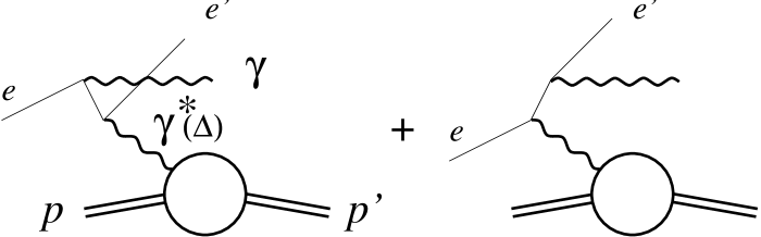
Figure 2: The Bethe-Heitler process.

We also introduce the angle $\varphi$ between the leptonic and hadronic scattering planes in the c.m. of the scattered photon and scattered proton (see Fig. 3). As we will show, the $\varphi$-dependence of the physical cross section contains a wealth of information. Rather than work at fixed $\varphi$ values — a procedure sometimes advocated to knock down the Bethe-Heitler contribution — we will show how to test the model using the full $\varphi$-dependence. Notice that with appropriate phase conventions for the external particles the contribution of VCS to the amplitude of (7) for a given helicity $\lambda$ of the intermediate photon $\gamma^{\ast}(q)$ has the $\varphi$-dependence

$${\cal T}_{\it VCS}\propto\exp(-i\lambda\varphi)\hskip 6.0pt,\hskip 6.0pt$$ (9)

which will allow us to find simple tests for the helicity structure of VCS.

Figure 3: Kinematics of reaction (7) in the c.m. of the scattered photon and proton.

Let us take a closer look at the BH process in the kinematic region where we want to test the handbag approximation, i.e. where $\Delta_{T}$, $\sqrt{-t}$ and $m$ are all small compared with $Q$. Since the handbag dominance holds in a $1/Q$ expansion, it is natural to also expand the BH amplitude in powers of $1/Q$. Its leading term goes like $\Delta_{T}/t$ or $m/t$, whereas ${\cal T}_{\it VCS}$ scales like $1/Q$ if the $\gamma^{\ast}p\to\gamma p$ amplitude behaves in $Q$ like a constant. This leads to a hierarchy in powers of $1/Q$ for the contributions to the $ep$ cross section of the squared BH amplitude, the VCS–BH interference and the squared VCS amplitude, respectively.

To understand the $\varphi$-dependence of the BH amplitude it is worth noting that the invariants $s^{\prime}=(k^{\prime}+q^{\prime})^{2}$ and $u^{\prime}=(k-q^{\prime})^{2}$, which appear in the lepton propagators at Born level, read

$$s^{\prime} = {Q^{2}\over y}-{2\Delta_{T}Q\sqrt{1-y}\over y}\cos\varphi+O(m^{2},t)\hskip 6.0pt,\hskip 6.0pt$$ (10)

$$u^{\prime} = -{Q^{2}\over y}(1-y)+{2\Delta_{T}Q\sqrt{1-y}\over y}\cos\varphi+O(m^{2},t)\hskip 6.0pt.\hskip 6.0pt$$ (11)

We see that $s^{\prime}$ and $u^{\prime}$ depend only weakly on $\varphi$ in the region of interest. Under the condition (8) we can expand in powers of $(\Delta_{T}/Q)\cdot\cos\varphi$ the propagators $1/s^{\prime}$ and $1/u^{\prime}$ in the expression of ${\cal T}_{\it BH}$, which gives at the same time a Fourier expansion in $\varphi$. To leading order in $1/Q$ we find a very simple $\varphi$-dependence:

$${\cal T}_{\it BH}\propto\exp(-2i\lambda^{\prime}\varphi)+O\left(1\over Q\right)$$ (12)

for a scattered photon of helicity $\lambda^{\prime}$.

We can now investigate the $\varphi$-dependence of the $ep$ cross section, with unpolarized protons and leptons for the time being. It is given by

$${d\sigma\over d\varphi\,dt\,dQ^{2}\,dx_{B}}=\frac{1}{32\,(2\pi)^{4}}\,\frac{x_{B}\,y^{2}}{Q^{4}}\,\frac{1}{\sqrt{1+4x_{B}^{2}m^{2}/Q^{2}}}\,|{\cal T}_{\it BH}+{\cal T}_{\it VCS}|^{2}\hskip 6.0pt.\hskip 6.0pt$$ (13)

The squared BH contribution has the structure

$$|{\cal T}_{\it BH}|^{2}=f_{1}(\epsilon,x_{B},\Delta_{T})+\frac{1}{Q}\cos\varphi\cdot f_{2}(\epsilon,x_{B},\Delta_{T})+O\left(1\over Q^{2}\right)\hskip 6.0pt,\hskip 6.0pt$$ (14)

with functions $f_{1}$ and $f_{2}$ whose expressions we do not need here. The square of VCS can readily be expressed in terms of helicity amplitudes $M^{\lambda,\lambda^{\prime}}_{h,h^{\prime}}(Q^{2},x_{B},\Delta_{T})$ for $\gamma^{\ast}p\to\gamma p$, where $\lambda$ ($\lambda^{\prime}$) is the helicity of the initial (final) state photon and $h$ ($h^{\prime}$) that of the initial (final) state proton. It reads

$$|{\cal T}_{\it VCS}|^{2} = \frac{e^{6}}{Q^{2}}\,\frac{2}{1-\epsilon}\,\sum_{h,h^{\prime}}\left[\>{1\over 2}\{|M^{1,1}_{h,h^{\prime}}|^{2}+|M^{-1,1}_{h,h^{\prime}}|^{2}\}+\epsilon\,|M^{0,1}_{h,h^{\prime}}|^{2}\right.$$ (15)

$${}-\cos\varphi\cdot\sqrt{\epsilon(1+\epsilon)}\,\mbox{Re}\{(M^{1,1}_{h,h^{\prime}})^{*}M^{0,1}_{h,h^{\prime}}-(M^{-1,1}_{h,h^{\prime}})^{*}M^{0,1}_{h,h^{\prime}}\}$$

$$\left.{}-\cos 2\varphi\cdot\epsilon\,\mbox{Re}\{(M^{1,1}_{h,h^{\prime}})^{*}M^{-1,1}_{h,h^{\prime}}\}\rule{0.0pt}{12.91663pt}\>\right]\hskip 6.0pt,\hskip 6.0pt$$

where $e$ is the electron charge. Finally, thanks to the simple $\varphi$-behavior in (9), (12) the BH–VCS interference can be written as

$${\cal T}_{\it BH}^{*}{\cal T}_{\it VCS}+{\cal T}_{\it VCS}^{*}{\cal T}_{\it BH} = \frac{e^{6}}{t}\,\frac{m}{Q}\cdot\frac{4\sqrt{2}}{x_{B}\sqrt{1-x_{B}}}\left[\cos\varphi\cdot\frac{1}{\sqrt{\epsilon(1-\epsilon)}}\,\mbox{Re}\tilde{M}^{1,1}\right.$$ (16)

$$\left.{}-\cos 2\varphi\cdot\sqrt{\frac{1+\epsilon}{1-\epsilon}}\,\mbox{Re}\tilde{M}^{0,1}-\cos 3\varphi\cdot\sqrt{\frac{\epsilon}{1-\epsilon}}\,\mbox{Re}\tilde{M}^{-1,1}\right]+O\left(1\over Q^{2}\right)\hskip 6.0pt,\hskip 6.0pt$$

for a negatively charged lepton. Here the $\gamma^{\ast}p\to\gamma p$ amplitudes enter in linear combinations

$$\tilde{M}^{\lambda,\lambda^{\prime}}(Q^{2},x_{B},\Delta_{T}) = \frac{\Delta_{T}}{m}\cdot\Big{[}(1-x_{B})\,G_{M}-(1-x_{B}/2)\,F_{2}\Big{]}\cdot M^{\lambda,\lambda^{\prime}}_{-1/2,-1/2}$$ (17)

$$+ \frac{\Delta_{T}}{m}\cdot\Big{[}G_{M}-(1-x_{B}/2)\,F_{2}\Big{]}\cdot M^{\lambda,\lambda^{\prime}}_{1/2,1/2}$$

$$+ \left[x_{B}^{2}\,G_{M}+\frac{\Delta_{T}^{2}}{2m^{2}}\,F_{2}\right]\cdot M^{\lambda,\lambda^{\prime}}_{1/2,-1/2}$$

$$- \frac{\Delta_{T}^{2}}{2m^{2}}\,F_{2}\cdot M^{\lambda,\lambda^{\prime}}_{-1/2,1/2}\hskip 6.0pt,\hskip 6.0pt$$

where $G_{M}$ is the magnetic and $F_{2}$ the Pauli form factor of the proton, both to be taken at momentum transfer $t$.

In summary, then, the hierarchy in powers of $1/Q$, with $|{\cal T}_{\it BH}|^{2}$, BH–VCS interference and $|{\cal T}_{\it VCS}|^{2}$ going like 1, $1/Q$ and $1/Q^{2}$, respectively, in the handbag model, is accompanied with a $\varphi$-distribution going like $\cos(n\varphi)$ with $n=0$, 1, 2 and 3. A powerful consequence is that extracting the angular distribution does not require any binning of data. One can instead weight the events with these angular functions, i.e. measure weighted cross sections

$$\langle\langle\,f(\varphi)\,\rangle\rangle=\frac{Q^{4}}{x_{B}\,y^{2}}\,\int d\varphi\,{d\sigma\over d\varphi\,dt\,dQ^{2}\,dx_{B}}\cdot f(\varphi)$$ (18)

with $f(\varphi)=1,\cos\varphi,\cos 2\varphi,\cos 3\varphi$, which directly project out the corresponding Fourier coefficients in the cross section. In $\langle\langle\,f(\varphi)\,\rangle\rangle$ we have taken out the factor $x_{B}\,y^{2}/Q^{4}$ from the phase space in (13) for later convenience. Other choices of weighting functions are possible: one can e.g. multiply the data by $\pm 1$ in alternating sectors, generalizing the concept of a left-right asymmetry, which is tantamount to choosing $f(\varphi)$ as the signature function of $\cos\varphi$, $\cos 2\varphi$, … Due to constraints from angular acceptance in a given experiment one may also have to choose functions $f(\varphi)$ that vanish in a certain range of $\varphi$. In any case one can use the statistics of the full data set to extract the Fourier coefficients of the cross section.

In (15) and (16) we note the very different $\epsilon$-dependence of the VCS and BH amplitudes: ${\cal T}_{\it VCS}$ has a relative factor of $1/\sqrt{1-\epsilon}$ compared with ${\cal T}_{\it BH}$. The numerical importance of ${\cal T}_{\it VCS}$ might thus be enhanced by exploiting the region close to $\epsilon=1$. At fixed $Q^{2}$ and $x_{B}$ this requires a large c.m. energy of the $ep$ reaction. Conversely, we note in the interference term (16) that small $\epsilon$ emphasizes the first term in the square brackets, going like $M^{1,1}_{h,h^{\prime}}$, which is one of the amplitudes we want to test.

Using the weighted cross sections (18) we now formulate a number of tests for the predictions of the handbag approximation. Let us first assume that $\epsilon$ is not too large so that the BH–VCS interference (16) dominates over the squared VCS amplitude (15) due to their respective global factors $1/Q$ and $1/Q^{2}$.

• We can test the scaling properties of the handbag: in the leading order interference term (16) the function $\cos\varphi$ is multiplied by the photon helicity conserving amplitudes $M^{1,1}_{h,h^{\prime}}$ which the handbag approximation predicts to be constant in $Q$. There is also a $\cos\varphi$-term in the square (14) of the BH amplitude, which has the same global power $1/Q$ and thus must be subtracted if we want to investigate VCS. Note that the BH process including its QED radiative corrections can be calculated and that the elastic proton form factors are well parameterized in the region of small $t$ where they are needed. We then have as a test for the scaling properties in the handbag that at fixed $\Delta_{T}$, $x_{B}$ and $y$

  $$\langle\langle\,\cos\varphi\,\rangle\rangle-\left.\langle\langle\,\cos\varphi\,\rangle\rangle\right._{\rm BH\ only}\sim 1/Q\hskip 6.0pt,\hskip 6.0pt$$ (19)

  where $\smash{\left.\langle\langle\,\cos\varphi\,\rangle\rangle\right._{\rm BH\ only}}$ denotes the contribution of the squared BH amplitude. Of course this scaling behavior is to be understood as up to logarithms due to QCD radiative corrections in the handbag.

  Note that with a fixed $ep$ c.m. energy the variables $x_{B}$, $y$ and $Q^{2}$ are not independent: changing $Q^{2}$ at fixed $x_{B}$ will change $y$. To investigate the $Q^{2}$-behavior of the amplitudes $M^{1,1}_{h,h^{\prime}}$ one must then multiply $\langle\langle\,\cos\varphi\,\rangle\rangle$ with an appropriate $\epsilon$-dependent factor to be taken from (16). A similar remark holds for the other weighted cross sections we will discuss.

  Beyond testing the handbag the measurement of $\langle\langle\,\cos\varphi\,\rangle\rangle$ should offer a good way to extract the leading twist VCS amplitudes, in a linear combination (17). This allows one to gain rather direct information on the new off-diagonal parton distributions if the handbag approximation is found to work well in a given kinematic regime.

• To test photon helicity conservation we can use $\langle\langle\,\cos 2\varphi\,\rangle\rangle$ and $\langle\langle\,\cos 3\varphi\,\rangle\rangle$. To order $1/Q$ they receive contributions from the BH–VCS interference proportional to $M^{0,1}_{h,h^{\prime}}$ and $M^{-1,1}_{h,h^{\prime}}$, respectively, which are zero in the handbag approximation and thus should be power suppressed. Note that $|{\cal T}_{\it BH}|^{2}$ does not contain any $\cos 2\varphi$ or $\cos 3\varphi$ up to order $1/Q$, so that, without needing to subtract this contribution, we have as a test for the handbag that

  $$\langle\langle\,\cos 2\varphi\,\rangle\rangle\hskip 6.0pt,\hskip 6.0pt\langle\langle\,\cos 3\varphi\,\rangle\rangle\sim 1/Q^{n}\hskip 6.0pt,\hskip 6.0ptn\geq 2\hskip 6.0pt.\hskip 6.0pt$$ (20)

  From (19) and (20) one has of course that $\langle\langle\,\cos 2\varphi\,\rangle\rangle$ and $\langle\langle\,\cos 3\varphi\,\rangle\rangle$ are small compared with $\langle\langle\,\cos\varphi\,\rangle\rangle$, a test that can even be done without much lever arm in $Q^{2}$.

  At the end of Sec. 3 we discussed the possibility of having leading twist amplitudes $M^{-1,1}_{h,h^{\prime}}$ at order $\alpha_{S}$ in the handbag. If such amplitudes exist then the behavior of $\langle\langle\,\cos 3\varphi\,\rangle\rangle$ should be like $\alpha_{S}/Q$ instead of the one given in (20).

Let us now see what can be done in the kinematic regime where $\epsilon$ is sufficiently close to 1 so that the VCS contribution to the amplitude dominates over the contribution from BH. It is then $|{\cal T}_{\it VCS}|^{2}$ that is dominant in the cross section.

• The scaling of the handbag can now be tested with the weighted cross section $\langle\langle\,1\,\rangle\rangle$: the constant part in the squared VCS amplitude (15) contains a term quadratic in the photon helicity conserving amplitudes $M^{1,1}_{h,h^{\prime}}$. We remark that the leading order interference term given in (16) does not contribute to $\langle\langle\,1\,\rangle\rangle$, but that the terms denoted by $O(1/Q^{2})$ there do contain a constant piece. By assumption it is suppressed compared with the contribution from $|{\cal T}_{\it VCS}|^{2}$, as well as the leading term in the squared BH amplitude (14), which one may but does not need to subtract. The scaling prediction of the handbag model is then

  $$\langle\langle\,1\,\rangle\rangle\sim 1/Q^{2}\hskip 6.0pt.\hskip 6.0pt$$ (21)

• $\langle\langle\,\cos 2\varphi\,\rangle\rangle$ is sensitive to the photon helicity changing amplitudes $M^{-1,1}_{h,h^{\prime}}$. The quark contribution in the handbag approximation gives

  $$\langle\langle\,\cos 2\varphi\,\rangle\rangle\sim 1/Q^{n}\hskip 6.0pt,\hskip 6.0ptn\geq 3\hskip 6.0pt,\hskip 6.0pt$$ (22)

  whereas the gluon diagrams could enhance this behavior by a factor $\alpha_{S}\cdot Q$. There is a corresponding test for the amplitudes $M^{0,1}_{h,h^{\prime}}$ involving $\langle\langle\,\cos\varphi\,\rangle\rangle$, but the contribution of the BH–VCS interference to this quantity is proportional to the leading twist amplitudes $M^{1,1}_{h,h^{\prime}}$, so that one will need smaller values of $(1-\epsilon)$ to suppress this contribution than in the case of $\langle\langle\,\cos 2\varphi\,\rangle\rangle$.

5. Let us now see which additional information on VCS can be gained using lepton beams with longitudinal polarization $h_{e}=\pm 1/2$, while still averaging over the proton spin. Recall that due to parity and time reversal invariance the $h_{e}$-dependent part of the cross section is the interference between the absorptive and the nonabsorptive part of the $ep$ scattering amplitude [13]. The BH amplitude is purely nonabsorptive at Born level. QED radiative corrections, although they can be sizeable, are not expected to significantly change this since a large part of them comes from the collinear and infrared regions which do not lead to large absorptive parts. As a consequence $|{\cal T}_{\it BH}|^{2}$ is independent of $h_{e}$. The $h_{e}$-dependent terms in the BH–VCS interference probe the absorptive part of VCS, i.e. $\mbox{Im}M^{\lambda,\lambda^{\prime}}_{h,h^{\prime}}$ with our phase conventions, while its $h_{e}$-independent part is sensitive only to $\mbox{Re}M^{\lambda,\lambda^{\prime}}_{h,h^{\prime}}$.

From parity invariance it follows that for unpolarized protons the $h_{e}$-dependent part of the cross section is odd in $\varphi$ and the $h_{e}$-independent part is even. The lepton spin asymmetry of the $\varphi$-integrated cross section is therefore zero, which might offer a useful experimental cross check for the lepton spin measurement and the acceptance in $\varphi$.

Compared with the lepton spin averaged expressions in (15), (16), we now have

$$|{\cal T}_{\it VCS}|^{2} = \left\{|{\cal T}_{\it VCS}|^{2}\right\}_{\rm eq.(\ref{VCSsquared})}+\frac{e^{6}}{Q^{2}}\,\frac{2}{1-\epsilon}\cdot$$ (23)

$$\sum_{h,h^{\prime}}2h_{e}\,\sin\varphi\cdot\sqrt{\epsilon(1-\epsilon)}\,\mbox{Im}\{(M^{1,1}_{h,h^{\prime}})^{*}M^{0,1}_{h,h^{\prime}}-(M^{-1,1}_{h,h^{\prime}})^{*}M^{0,1}_{h,h^{\prime}}\}$$

and

$${\cal T}_{\it BH}^{*}{\cal T}_{\it VCS}+{\cal T}_{\it VCS}^{*}{\cal T}_{\it BH} = \left\{{\cal T}_{\it BH}^{*}{\cal T}_{\it VCS}+{\cal T}_{\it VCS}^{*}{\cal T}_{\it BH}\right\}_{\rm eq.(\ref{interference})}+\frac{e^{6}}{t}\,\frac{m}{Q}\cdot\frac{4\sqrt{2}}{x_{B}\sqrt{1-x_{B}}}\cdot$$ (24)

$$2h_{e}\left[-\sin\varphi\cdot\sqrt{\frac{1+\epsilon}{\epsilon}}\,\mbox{Im}\tilde{M}^{1,1}+\sin 2\varphi\cdot\mbox{Im}\tilde{M}^{0,1}\right]+O\left(1\over Q^{2}\right)\hskip 6.0pt.\hskip 6.0pt$$

Note the absence of $\sin 3\varphi$ in the interference term and of $\sin 2\varphi$ in $|{\cal T}_{\it VCS}|^{2}$. We can now complete our list of tests for the handbag by considering two more weighted cross sections, starting again with the region of $\epsilon$ where the BH–VCS interference dominates over the square of VCS :

• $\langle\langle\,\sin\varphi\,\rangle\rangle$ is analogous to $\langle\langle\,\cos\varphi\,\rangle\rangle$ discussed above, with the difference that now no subtraction of $|{\cal T}_{\it BH}|^{2}$ is necessary. The scaling prediction of the handbag is

  $$\langle\langle\,\sin\varphi\,\rangle\rangle\sim 1/Q\hskip 6.0pt.\hskip 6.0pt$$ (25)

  We emphasize again that $\langle\langle\,\sin\varphi\,\rangle\rangle$ and $\smash{\left.\langle\langle\,\cos\varphi\,\rangle\rangle-\langle\langle\,\cos\varphi\,\rangle\rangle\right._{\rm BH\ only}}$ offer a way to extract the imaginary and real parts of the $M^{\lambda,\lambda^{\prime}}_{h,h^{\prime}}$ separately. This is a great advantage of the interference term compared with $|{\cal T}_{\it VCS}|^{2}$, where real and imaginary parts mix and should be difficult to disentangle. Remember that owing to P and T invariance the off-diagonal parton distributions introduced in [2] are real valued, so that $\smash{\mbox{Im}M^{\lambda,\lambda^{\prime}}_{h,h^{\prime}}}$ is given by the off-diagonal distributions at $x=x_{B}$ and $x^{\prime}=0$ and $\smash{\mbox{Re}M^{\lambda,\lambda^{\prime}}_{h,h^{\prime}}}$ by a principal value integral over $x$. Separating the real and imaginary parts of $\smash{M^{\lambda,\lambda^{\prime}}_{h,h^{\prime}}}$ is crucial to obtain detailed information on the new parton distributions.

• $\langle\langle\,\sin 2\varphi\,\rangle\rangle$ only receives contributions from the interference. As $\langle\langle\,\cos 3\varphi\,\rangle\rangle$ and $\langle\langle\,\cos 2\varphi\,\rangle\rangle$ it can be used to test for photon helicity conservation, the handbag prediction being

  $$\langle\langle\,\sin 2\varphi\,\rangle\rangle\sim 1/Q^{n}\hskip 6.0pt,\hskip 6.0ptn\geq 2\hskip 6.0pt.\hskip 6.0pt$$ (26)

  We should remark that these quantities test for different photon helicity changing amplitudes and are thus not redundant: $\langle\langle\,\sin 2\varphi\,\rangle\rangle$ is sensitive to $\mbox{Im}M^{0,1}_{h,h^{\prime}}$, $\langle\langle\,\cos 2\varphi\,\rangle\rangle$ to $\mbox{Re}M^{0,1}_{h,h^{\prime}}$, and $\langle\langle\,\cos 3\varphi\,\rangle\rangle$ to $\mbox{Re}M^{-1,1}_{h,h^{\prime}}$.

For large $\epsilon$ where the square of VCS dominates the cross section one might use $\langle\langle\,\sin\varphi\,\rangle\rangle$ to test for the amplitudes $M^{0,1}_{h,h^{\prime}}$, with the same caveat concerning the BH–VCS interference contribution we have made for $\langle\langle\,\cos\varphi\,\rangle\rangle$ in the previous section.

We finally remark that the measurement of $\langle\langle\,\sin\varphi\,\rangle\rangle$ and $\langle\langle\,\sin 2\varphi\,\rangle\rangle$ does not require us to form a lepton spin asymmetry. In fact, all moments (19) – (22) and (25) – (26) can be determined independently with just one nonzero value of the lepton polarization.

6. We have shown how the photon spin structure of $\gamma^{\ast}p\to\gamma p$ can be investigated using the distribution of the angle $\varphi$, both with and without lepton polarization. To measure the dependence of $M^{\lambda,\lambda^{\prime}}_{h,h^{\prime}}$ on the proton helicities $h$, $h^{\prime}$ one needs an experiment with proton polarization. A different class of tests of the handbag dominance can be built along the lines drawn in the present study.

We shall not elaborate on this subject here, but just illustrate what are the additional possibilities brought by the extra degree of freedom, focusing on the amplitudes where the proton changes its helicity. A possibility to extract information on these amplitudes is offered by a transversely polarized proton target, the transverse spin asymmetry being given by the interference of proton helicity flip with helicity no-flip amplitudes. In the handbag model the proton helicity flip amplitudes have a factor $\Delta_{T}R_{p}$ as mentioned in Sec. 3. That is, they are linear in $\Delta_{T}$ for $\Delta_{T}\to 0$ as required by angular momentum conservation for amplitudes where the photon helicity does not change. In general there is however an amplitude $M^{0,1}_{1/2,-1/2}$, which can be finite at $\Delta_{T}=0$ since both proton and photon change spin by one unit. This amplitude is zero in the handbag because the photon is longitudinal. We then have as a further prediction that to leading order in $1/Q$ proton helicity flip amplitudes must vanish like $\Delta_{T}$ as $\Delta_{T}$ goes to zero.

Acknowledgments.
We gratefully acknowledge discussions with Mauro Anselmino, John Collins, Pierre Guichon, Peter Kroll, Peter Landshoff, Wei Lu and Otto Nachtmann. T. G. was carrying out his work as part of a training Project of the European Community under Contract No. ERBFMBICT950411. This work has been partially funded through the European TMR Contract No. FMRX-CT96-0008: Hadronic Physics with High Energy Electromagnetic Probes, and through DOE grant No. 85ER40214.

References

- [1] S.J. Brodsky, F. Close and J.F. Gunion, Phys. Rev. D6 (1972) 177.
- [2] X. Ji, Phys. Rev. Lett. 78 (1997) 610; Phys. Rev. D55 (1997) 7114.
- [3] A.V. Radyushkin, Phys. Lett. B380 (1996) 417; Phys. Lett. B385 (1996) 333.
- [4] C. Hyde-Wright, in: Proceedings of the second ELFE workshop, Saint Malo, France, 1996, eds. N. d’Hose et al., to be published in Nucl. Phys. A (1997).
-
[5]
B. Geyer et al., Z. Phys. C26 (1985) 591;
T. Braunschweig et al., Z. Phys. C33 (1987) 275;
F.-M. Dittes et al., Phys. Lett. B209 (1988) 325;
I.I. Balitskii and V.M. Braun, Nucl. Phys. B311 (1988/89) 541;
P. Jain and J.P. Ralston, in: Future Directions in Particle and Nuclear Physics at Multi-GeV Hadron Beam Facilities, BNL, March 1993;
X. Ji, W. Melnitchouk and X. Song, hep-ph/9702379;
P. Hoodbhoy, hep-ph/9703365;
L. Frankfurt et al., hep-ph/9703449. - [6] X. Ji, J. Tang and P. Hoodbhoy, Phys. Rev. Lett. 76 (1996) 740.
- [7] K. Watanabe, Prog. Theor. Phys. 67 (1982) 1834.
- [8] Z. Chen, hep-ph/9705279.
- [9] A. Afanasev, hep-ph/9608305.
-
[10]
Workshop on CEBAF at Higher Energies, CEBAF, April
1994;
Hermes proposal, Report DESY-PRC 90/01;
G. Baum et al., COMPASS: A proposal for a common muon and proton apparatus for structure and spectroscopy, CERN-SPSLC-96-14 (1996);
The ELFE Project, eds. J. Arvieux and E. De Sanctis, Conference Proceedings, Vol. 44, Italian Physical Society, Bologna 1993;
J. Arvieux and B. Pire, Progress in Particle and Nuclear Physics 30 (1995) 299. - [11] R.G. Roberts, The Structure of the Proton, Cambridge Univ. Press, Cambridge 1990.
-
[12]
G.R. Farrar and H. Zhang, Phys. Rev. Lett. 65
(1990) 1721; Phys. Rev. D41 (1990) 3348;
G.R. Farrar and E. Maina, Phys. Lett. B206 (1988) 120;
A.S. Kronfeld and B. Nižić, Phys. Rev. D44 (1991) 3445. - [13] P. Kroll, M. Schürmann and P.A.M. Guichon, Nucl. Phys. A598 (1996) 435.
- [14] M.G. Sotiropoulos and G. Sterman, Nucl. Phys. B425 (1994) 489.
- [15] G.R. Farrar and G. Sterman, Phys. Rev. Lett. 62 (1989) 2229.
- [16] P.A.M. Guichon, G.Q. Liu and A.W. Thomas, Nucl. Phys. A591 (1995) 606.