Improving constraints on $\tan\beta/m_{H}$ using $B$$\to$$D\tau\overline{\nu}$

Abstract

We study the $q^{2}$ dependence of the exclusive decay mode $B$$\to$$D\tau\overline{\nu}$ in type II two Higgs doublet models and show that this mode may be used to put stringent bounds on $\tan\beta/m_{H}$. There are currently rather large theoretical uncertainties in the $q^{2}$ distribution, but these may be significantly reduced by future measurements of the analogous distribution for $B$$\to$$D(e,\mu)\overline{\nu}$. We estimate that this reduction in the theoretical uncertainties would eventually (i.e., with sufficient data) allow one to push the upper bound on $\tan\beta/m_{H}$ down to about $0.06$ GeV^-1. This would represent an improvement on the current bound by about a factor of $7$. We then apply the method of optimized observables which allows us to estimate the reach of an experiment with a given number of events. We thus find that an experiment with, for example, $10^{3}$ events could set a $2\sigma$ upper bound on $\tan\beta/m_{H}$ of $0.07$ GeV^-1 or could differentiate at the $4.6\sigma$ level between a 2HDM with $\tan\beta/m_{H}=0.1$ GeV^-1 and the SM.

I Introduction

There has recently been considerable interest in constraining the parameter space of type II two Higgs doublet models. The main reason for this interest, of course, is that the Higgs sectors of minimal supersymmetric extensions of the standard model are generically of this type [1]. The charged Higgs sectors of two Higgs doublet models (2HDM’s) may be characterized by the ratio of the two Higgs’ vacuum expectation values, $\tan\beta$, and the mass of the charged Higgs, $m_{H}$. In this work we will investigate how the exclusive decay channel $B\to D\tau\overline{\nu}$ may be used to place tight constraints on the ratio $\tan\beta/m_{H}$. This channel is expected to have a branching ratio on the order of half a percent [2], so that one would expect on the order of $10^{6}$ such decays at the $B$ factories which are currently under construction.

There already exist several constraints on $\tan\beta$ and $m_{H}$. The most direct lower bound on the charged Higgs mass comes from the non-observation of charged Higgs pairs in $Z$ decays and gives $m_{H}>44$ GeV [3]. Another limit comes from top decays, which yield the bound $m_{H}>147$ GeV for large $\tan\beta$ [4]. Finally, for pure type II 2HDM’s one finds $m_{H}>300$ GeV, coming from the virtual Higgs contributions to $b\to s\gamma$ [5]. This latter limit disappears in the context of supersymmetry since the Higgs contributions to $b\to s\gamma$ can be cancelled by other contributions [6]. There are no experimental upper bounds on the mass of the charged Higgs, but one generally expects to have $m_{H}<1$ TeV in order that perturbation theory remain valid [7]. A lower limit may be placed on $\tan\beta$ by considering the branching ratio for $Z\to b\overline{b}$. The resulting bound of $\tan\beta>0.7$, obtained in Ref. [8], coincides with the range generally favoured by theorists in order that renormalization group evolution drive electroweak symmetry breaking [10]. For large $\tan\beta$ the most stringent constraints on $\tan\beta$ and $m_{H}$ are actually on their ratio, $\tan\beta/m_{H}$. The current limits come from the measured branching ratio for the inclusive decay $B\to X\tau\overline{\nu}$, giving $\tan\beta/m_{H}<0.46$ GeV^-1 [11], and from the upper limit on the branching ratio for $B\to\tau\overline{\nu}$, giving $\tan\beta/m_{H}<0.38$ GeV^-1 [12]. While both of these limits are quoted as being at the $90\%$ confidence level, the latter may be somewhat less constraining due to the uncertainties in $V_{ub}$ and $f_{B}$.

Our main goal in this paper is to investigate the sensitivity of the exclusive decay $B\to D\tau\overline{\nu}$ to the ratio $\tan\beta/m_{H}$. We will concentrate on the $q^{2}$ distribution for this decay and discuss how the theoretical uncertainties in this distribution may be minimized. We also apply the optimized weighting procedure [13, 14] to this distribution in order to derive quantitative estimates for the sensitivities of experiments with given numbers of events. This procedure can be shown to give the smallest statistical uncertainty when analyzing the data in a given experiment. The present work complements the previous theoretical studies of the inclusive [15, 16, 17, 18, 19, 20, 21, 22] and exclusive [23, 24] semi-tauonic $B$ decays, as well as those of the purely leptonic decays $B\to\tau\overline{\nu}$ [18] and $B_{c}\to\tau\overline{\nu}$ [25]. These decays are attractive because the Higgs contribution occurs at tree-level and cannot be cancelled by, for example, supersymmetric loop effects. Thus, the results of our analysis should be applicable to any type II 2HDM [26] This situation may be contrasted with that in $b\to s\gamma$ [6].

A feature which is common to all of the tauonic and semi-tauonic $B$ decays is that the Higgs contribution to the amplitude interferes destructively with that due to the standard model (SM). As a result, the corresponding integrated partial widths, plotted as functions of $\tan\beta/m_{H}$, tend to have minima around $\tan\beta/m_{H}\sim 0.2$ – $0.3$ GeV^-1. Most studies to date have concentrated on the region to the right of the minimum, where the Higgs contribution to the width begins to dominate over the SM contribution. Indeed, the present experimental limits – derived using integrated partial widths – correspond to this region. In order to use semi-tauonic decays to probe values of $\tan\beta/m_{H}$ near and/or below the minimum, it will be extremely useful to have detailed theoretical predictions for quantities beyond simply the integrated partial widths. This is because the plots of the widths as functions of $\tan\beta/m_{H}$ are generically relatively flat up to $\tan\beta/m_{H}\sim 0.4$ GeV^-1. Several authors have suggested using the energy distribution or longitudinal polarization of the $\tau$ in this regard, but this may be difficult experimentally since two neutrinos are always lost. An alternative approach, which we will study in detail, is to use the $q^{2}$ distribution. A possible drawback of this approach is that the $q^{2}$ distribution is very sensitive to theoretical uncertainties in the shapes of the hadronic form factors. As we shall see, however, the situation in the exclusive channel $B\to D\tau\overline{\nu}$ appears to be quite encouraging. The reason for this is that once the distribution for $B\to D(e,\mu)\overline{\nu}$ has been measured, that for $B\to D\tau\overline{\nu}$ can be predicted with relatively small theoretical uncertainties. The resulting distribution is quite sensitive to $\tan\beta/m_{H}$, even for relatively small values of this ratio. Furthermore, the $q^{2}$ distribution has a qualitatively different shape for values of $\tan\beta/m_{H}$ above and below the “critical value”, $\tan\beta/m_{H}\sim 0.3$ GeV^-1.

We have chosen to focus on the decay channel $B\to D\tau\overline{\nu}$ instead of on $B\to D^{*}\tau\overline{\nu}$, even though the latter channel will likely have a somewhat larger branching ratio and may also be more accessible experimentally (in analogy with the decays to the lighter leptons [27]) than the former. Our main motivation for considering $B\to D\tau\overline{\nu}$ rather than $B\to D^{*}\tau\overline{\nu}$ is simply that the Higgs contribution has a much larger effect in the former case. This feature has already been noted in Ref. [24] and is in part due to an enhancement by a factor $(m_{B}+m_{D})/(m_{B}-m_{D})\sim 2$ in the effective interaction. As noted in Ref. [24], this enhancement effect means that the exclusive $D$ channel is also more sensitive than the inclusive channel, since the less-sensitive $D^{*}$ mode tends to dilute the inclusive measurement.

The plan of the remainder of this paper is as follows. We begin in Sec. II by deriving the $q^{2}$ distribution for $B\to D\tau\overline{\nu}$ in terms of the dimensionless variable $t=q^{2}/m_{B}^{2}$. In Sec. III we estimate the theoretical uncertainties in this distribution and in the integrated width once the distribution for $B\to D(e,\mu)\overline{\nu}$ has been measured. Barring any further input, these uncertainties would eventually limit the reach of such an experiment. In Sec. IV we apply the optimized weighting procedure to the $q^{2}$ distribution and in Sec. V we present our conclusions.

II Calculation of the differential distribution

The two diagrams which contribute to the decay $B$$\to$$D\tau\overline{\nu}$ in a type II 2HDM are shown in Fig. 1. The amplitude corresponding to the SM $W$-exchange diagram (Fig. 1(a)) is given by

$${\cal M}_{\rm SM}=-2\sqrt{2}G_{F}V_{cb}\langle D(p^{\prime})|\overline{c}_{L}\gamma^{\mu}b_{L}|B(p)\rangle\overline{\tau}_{L}(p_{\tau})\gamma_{\mu}\nu_{L}(p_{\nu}),$$ (1)

where $\psi_{L}$$\equiv$$\frac{1}{2}(1-\gamma^{5})\psi$. The matrix element of the axial vector current in the above expression is identically zero since one cannot form an axial vector using only $p$ and $p^{\prime}$. The vector current matrix element may be expressed in terms of two form factors, $F_{0}$ and $F_{1}$, which are defined as follows:

$$\langle D(p^{\prime})|\overline{c}\gamma^{\mu}b|B(p)\rangle=F_{1}(t)\left[(p+p^{\prime})^{\mu}-\frac{m_{B}^{2}-m_{D}^{2}}{q^{2}}q^{\mu}\right]+F_{0}(t)\frac{m_{B}^{2}-m_{D}^{2}}{q^{2}}q^{\mu},$$ (2)

with $q=p-p^{\prime}$ and $t=q^{2}/m_{B}^{2}$. The form factors $F_{0}$ and $F_{1}$ are normalized such that $F_{0}(0)$$=$$F_{1}(0)$. There is thus no singularity at $q^{2}$$=$$0$.

The parametrization of the form factors given in Eq. (2) is particularly well-suited for our purposes since $F_{0}(t)$ and $F_{1}(t)$ may be associated with the spin-0 and spin-1 components of the exchange particles, respectively [28]. The contribution to the total amplitude coming from the (spin-0) charged Higgs diagram (Fig. 1(b)) may then be included by the following replacement in the SM expression for the amplitude:

$$F_{0}(t)\rightarrow F_{0}(t)\left(1+\delta_{H}(t)\right).$$ (3)

The function $\delta_{H}(t)$ is given by

$$\delta_{H}(t)=-\left(\frac{\tan\beta}{m_{H}}\right)^{2}\frac{m_{b}m_{B}^{2}t}{(m_{B}-m_{D})}\left(1+\frac{m_{c}}{m_{b}}\cot^{2}\beta\right)\frac{F_{S}(t)}{F_{0}(t)},$$ (4)

where the scalar form factor $F_{S}(t)$ is defined by

$$\langle D(p^{\prime})|\overline{c}b|B(p)\rangle=(m_{B}+m_{D})F_{S}(t).$$ (5)

It is now straightforward to work out the expression for the differential partial width in terms of these form factors. Let us first define the following dimensionless quantities:

$$r_{D}=\frac{m_{D}^{2}}{m_{B}^{2}}\;,\;\;\;\;\;r_{\tau}=\frac{m_{\tau}^{2}}{m_{B}^{2}}\;.$$ (6)

The expression for the width is then

$$\frac{d\Gamma(B\to D\tau\overline{\nu})}{dt}=\frac{G_{F}^{2}|V_{cb}|^{2}m_{B}^{5}}{128\pi^{3}}\rho(t),$$ (7)

where the dimensionless Dalitz density, $\rho(t)$, may be decomposed into spin-0 and spin-1 contributions as follows,

$$\rho(t)=\left(1+\delta_{H}(t)\right)^{2}\rho_{0}(t)+\rho_{1}(t),$$ (8)

with

$$\rho_{0}(t) = \frac{r_{\tau}}{t}\left[F_{0}(t)\right]^{2}\left(1-\frac{r_{\tau}}{t}\right)^{2}(1-r_{D})^{2}\lambda^{\frac{1}{2}}(1,r_{D},t),$$ (9)

$$\rho_{1}(t) = \frac{2}{3}\left[F_{1}(t)\right]^{2}\left(1-\frac{r_{\tau}}{t}\right)^{2}\left(1+\frac{r_{\tau}}{2t}\right)\lambda^{\frac{3}{2}}(1,r_{D},t),$$ (10)

and

$$\lambda(a,b,c)=a^{2}+b^{2}+c^{2}-2(ab+ac+bc).$$ (11)

The above expression for the differential width is a sum of two semi-positive definite terms, corresponding separately to the spin-0 and spin-1 contributions. The spin-0 contribution disappears in the limit $r_{\tau}$$\to$$0$, so that in this limit we recover the familiar expression for the semileptonic decay to an electron or muon. This observation is actually very important, since the distribution $d\Gamma_{(e,\mu)}/dt$ is expected to be measured very precisely at the $B$ factories which are currently under construction. Such a measurement would yield valuable information regarding the distribution $d\Gamma_{(\tau)}/dt$, since

$$\frac{d\Gamma_{(\tau)}}{dt}=\frac{d\Gamma_{(e,\mu)}}{dt}\left(1-\frac{r_{\tau}}{t}\right)^{2}\left[\left(1+\frac{r_{\tau}}{2t}\right)+\frac{3r_{\tau}}{2t}\frac{(1-r_{D})^{2}}{\lambda(1,r_{D},t)}\zeta^{2}(t)\left(1+\delta_{H}(t)\right)^{2}\right],$$ (12)

where $r_{\tau}\leq t\leq\left(1-\sqrt{r_{D}}\right)^{2}$ and

$$\zeta(t)\equiv\frac{F_{0}(t)}{F_{1}(t)}.$$ (13)

Thus, the measurement of the differential distribution for the decays $B\to D(e,\mu)\overline{\nu}$ may be used to predict the SM distribution for the decay into the $\tau$, up to the function $\zeta(t)$. As we shall see in the next section, $\zeta(t)$ may be calculated within the context of Heavy Quark Effective Theory with a relatively small uncertainty.

In the remainder of this work we examine the $t$ distribution in Eq. (7) in detail and evaluate its sensitivity to a Higgs signal.

III Theoretical uncertainties in the rate and in the differential distribution

Our goal in this section is to estimate the theoretical uncertainties in the distribution $d\Gamma_{(\tau)}/dt$ and in the integrated width if the analogous distribution $d\Gamma_{(e,\mu)}/dt$ has been measured very accurately. The first step is to evaluate the form factors $F_{0}$, $F_{1}$ and $F_{S}$ in the heavy quark symmetry limit using the results of Heavy Quark Effective Theory (HQET). Since in this limit all of the form factors have a known dependence on a single universal function – the Isgur-Wise function [29] – one is potentially in very good shape for trying to disentangle the Higgs contribution from the SM contribution in the $t$ distribution. The symmetry-breaking corrections to this picture introduce theoretical uncertainties into the calculation of the function $\zeta(t)=F_{0}(t)/F_{1}(t)$. It is this function which determines the shape of the distribution $d\Gamma_{(\tau)}/dt$ and whose uncertainties we shall need to estimate.

It is natural in the context of HQET to define quantities in terms of the meson velocities instead of in terms of their momenta. The matrix element of the hadronic vector current is then usually written as

$$\langle D(v^{\prime})|\overline{c}\gamma^{\mu}b|B(v)\rangle=\sqrt{m_{B}m_{D}}\left[h_{+}(w)(v+v^{\prime})^{\mu}+h_{-}(w)(v-v^{\prime})^{\mu}\right],$$ (14)

where $v^{\mu}$$=$$p^{\mu}/m_{B}$, $v^{\prime\mu}$$=$$p^{\prime\mu}/m_{D}$ and

$$w\equiv v\cdot v^{\prime}=\frac{1+r_{D}-t}{2\sqrt{r_{D}}}.$$ (15)

Comparing the expressions in Eqs. (14) and (2), we find the (exact) correspondence

$$F_{0}(t) = -\frac{1}{2\,r_{D}^{1/4}}\left[\left(\frac{t-(1+\sqrt{r_{D}})^{2}}{1+\sqrt{r_{D}}}\right)h_{+}(w)-\left(\frac{t-(1-\sqrt{r_{D}})^{2}}{1-\sqrt{r_{D}}}\right)h_{-}(w)\right],$$ (16)

$$F_{1}(t) = \frac{1}{2\,r_{D}^{1/4}}\left[(1+\sqrt{r_{D}})h_{+}(w)-(1-\sqrt{r_{D}})h_{-}(w)\right].$$ (17)

The formalism of HQET gives a self-consistent way to express hadronic form factors in an expansion in powers of $\Lambda/m_{Q}$, where $m_{Q}$ represents the masses of the heavy quarks involved in the transition and where $\Lambda$ represents a dimensionful quantity which is generically of order $\Lambda_{\rm QCD}$. For the meson form factors the first-order corrections are proportional to $\overline{\Lambda}/m_{Q}$, where $\overline{\Lambda}$ is defined as the difference between the meson and quark masses:

$$\overline{\Lambda}=M_{M}-m_{Q}.$$ (18)

To leading order in the $1/m_{Q}$ expansion all of the form factors may be expressed in terms of the universal Isgur-Wise function, $\xi(w)$, which satisfies the normalization condition $\xi(1)$$=$$1$. In the heavy quark symmetry limit, and ignoring short-distance QCD corrections, one finds that $h_{+}(w)$$\to$$\xi(w)$ and $h_{-}(w)$$\to$$0$, so that

$$F_{0}(t) \stackrel{{\scriptstyle HQS}}{{\longrightarrow}} -\frac{1}{2\,r_{D}^{1/4}}\left(\frac{t-(1+\sqrt{r_{D}})^{2}}{1+\sqrt{r_{D}}}\right)\xi(w),$$ (19)

$$F_{1}(t) \stackrel{{\scriptstyle HQS}}{{\longrightarrow}} \frac{1+\sqrt{r_{D}}}{2\,r_{D}^{1/4}}\xi(w).$$ (20)

Similar considerations for the scalar matrix element yield

$$F_{S}(t)\stackrel{{\scriptstyle HQS}}{{\longrightarrow}}F_{0}(t).$$ (21)

The above expressions receive corrections due to the finite masses of the heavy quarks. The $1/m_{Q}$ corrections to $h_{\pm}$ have been considered in detail in Ref. [27], while the corrections to the scalar matrix element do not appear to have been calculated. For this reason we will, for the purpose of estimating the theoretical errors, take the relation in Eq. (21) to be exact. This will not lead to significant errors in attempting to bound small values of $\tan\beta/m_{H}$. Under this assumption, $\delta_{H}(t)$ takes the simple form

$$\delta_{H}(t)\simeq-\left(\frac{\tan\beta}{m_{H}}\right)^{2}\frac{m_{b}m_{B}^{2}t}{(m_{B}-m_{D})},$$ (22)

where we have also dropped the term proportional to $m_{c}$, since its contribution to the amplitude is typically very small for the range of $\tan\beta$ which we will be considering.

The form factors $h_{\pm}$ receive both short- and long-distance corrections. The short-distance corrections are embodied in the Wilson coefficients and may be calculated reliably using perturbation theory and renormalization group evolution. They typically give corrections to the tree-level results which are on the order of $10\%$ [27]. The long-distance corrections are intrinsically non-perturbative and give rise to new sub-leading universal functions. At order $1/m_{Q}$ there are four such functions [30]. The corrections to the results obtained in the heavy quark symmetry limit may be taken into account by writing

$$h_{\pm}(w)\equiv N_{\pm}(w)\xi_{\rm ren}(w),$$ (23)

where the renormalized Isgur-Wise function is defined such that it still satisfies $\xi_{\rm ren}(1)$$=1$. The explicit expressions for $N_{\pm}$ to order $1/m_{Q}$ may be found in Ref. [27]. Their values at zero recoil ($w$$=$$1$) are of particular interest since one may use this information to extract $V_{cb}$ from the differential distribution for $B\to D(e,\mu)\overline{\nu}$. It is known that $N_{+}$ is protected by Luke’s theorem [30] and thus does not receive any $1/m_{Q}$ corrections at zero recoil. $N_{-}$ does receive $1/m_{Q}$ corrections at zero recoil, but the resulting contributions to the decay rate are parametrically suppressed by the factor $[(m_{B}-m_{D})/(m_{B}+m_{D})]^{2}\sim 0.23$ [31, 32, 33]. The uncertainties in the decay rate at zero recoil due to $N_{-}$ are thus on the order of a few percent, which is about the same size as the expected $1/m_{Q}^{2}$ corrections.

We are now in a position to calculate the function $\zeta(t)$, the ratio of $F_{0}$ and $F_{1}$, which appears in the expression for the differential distribution given in Eq. (12). Since $|N_{-}|$$\ll$$|N_{+}|$, as will be clear a posteriori, it is an excellent approximation to expand $\zeta(t)$ in powers of $N_{-}/N_{+}$. To first order this gives

$$\zeta(t)\simeq\zeta_{\infty}(t)+\frac{4t\sqrt{r_{D}}}{(1-r_{D})(1+\sqrt{r_{D}})^{2}}\frac{N_{-}(w)}{N_{+}(w)},$$ (24)

where

$$\zeta_{\infty}(t)=\frac{(1+\sqrt{r_{D}})^{2}-t}{(1+\sqrt{r_{D}})^{2}}$$ (25)

is the result obtained in the limit of heavy quark symmetry.

The theoretical error associated with $\zeta(t)$ is actually remarkably small. The main reason for this is that there is an approximate accidental cancellation in the expression for $N_{-}$ which tends to make it a very small number, to leading order in $1/m_{Q}$ [27]. The resulting uncertainties due to our ignorance of the forms of the sub-leading universal functions tend then also to be small (on the order of several percent). By way of contrast, the uncertainties in $N_{+}$ are rather large (on the order of $20\%$), but these have a negligible effect on the ratio $N_{-}/N_{+}$. This means that while the current predictions for $F_{0}(t)$ and $F_{1}(t)$ have large theoretical uncertainties, the prediction for the ratio of $F_{0}(t)$ and $F_{1}(t)$ has a relatively small theoretical uncertainty. Thus, once $F_{1}(t)$ has been determined experimentally, $F_{0}(t)$ is also known quite well. The ratio $N_{-}/N_{+}$ may be estimated by using the forms predicted for the sub-leading functions in specific model calculations. These functions have been calculated using QCD sum rules in Refs. [32, 33, 27]. We have studied $N_{-}/N_{+}$ numerically by allowing the sub-leading functions to vary over the regions suggested in the plots in Ref. [27] and by allowing $\overline{\Lambda}$ to vary in the range

$$0.4\;{\rm GeV}\leq\overline{\Lambda}\leq 0.6\;{\rm GeV}.$$ (26)

We have, for consistency, taken the heavy quark masses to be defined in terms of $\overline{\Lambda}$ through Eq. (18), setting $m_{b}=4.8$ GeV and $m_{c}=1.45$ GeV when $\overline{\Lambda}=0.5$ GeV. The resulting range for $N_{-}/N_{+}$ is then given by $-0.06\leq N_{-}(w)/N_{+}(w)\leq 0.0$, for $1.0\leq w\leq 1.6$. In order to account for the unknown $1/m_{Q}^{2}$ corrections, we conservatively double the size of this region. We thus estimate the range of theoretical uncertainty in $N_{-}/N_{+}$ to be

$$-0.09\leq\frac{N_{-}(w)}{N_{+}(w)}\leq 0.03.$$ (27)

It is now straightforward to use Eq. (12) to determine the differential width for $B\to D\tau\overline{\nu}$ once that for $B\to D(e,\mu)\overline{\nu}$ is known. The resulting curve will have a theoretical uncertainty determined by the uncertainty in the ratio $N_{-}/N_{+}$. We illustrate this procedure in Fig. 2 by plotting $(1+\delta_{H}(t))^{2}\rho_{0}(t)$ (shaded bands) and $\rho_{1}(t)$ (solid line) for the SM and for 2HDM’s with $\tan\beta/m_{H}=0.06$, $0.25$, and $0.35$ GeV^-1. The spin-1 contribution to the width, $\rho_{1}(t)$, is independent of $\tan\beta/m_{H}$ and is assumed to have been determined experimentally from the decays to the lighter leptons. The spin-0 contribution, $(1+\delta_{H}(t))^{2}\rho_{0}(t)$, is determined from the spin-1 contribution by using the relation $F_{0}(t)=\zeta(t)F_{1}(t)$, with $\zeta(t)$ as given in Eq. (24). For the purposes of this plot we have used the simple heavy quark symmetry relation for $F_{1}(t)$ given in Eq. (20), taking $\xi(w)=1-0.75\times(w-1)$. Note that the spin-0 contribution is qualitatively quite different for $\tan\beta/m_{H}=0.25$ GeV^-1 and $\tan\beta/m_{H}=0.35$ GeV^-1. These values fall on either side of the “critical value”, $\tan\beta/m_{H}\sim 0.3$ GeV^-1, for which the integrated width is at a minimum. From this plot we estimate that the current theoretical uncertainty would allow one to use the differential distribution in $B\to D\tau\overline{\nu}$ to rule out a 2HDM with $\tan\beta/m_{H}>0.06$ GeV^-1.

It is also useful to examine the behaviour of the integrated width as a function of $\tan\beta/m_{H}$. This behaviour is illustrated in Fig. 3 in terms of the dimensionless quantity $\overline{\rho}\equiv\int\rho(t)dt$, which is normalized by the factor $G_{F}^{2}|V_{cb}|^{2}m_{B}^{5}/128\pi^{3}$ (see Eq. (7)). As in Fig. 2, the shaded band corresponds to the theoretical uncertainty in the ratio $\zeta(t)=F_{0}(t)/F_{1}(t)$ and does not include the uncertainty in the form factor $F_{S}(t)$. For the sake of illustration we have again used the simple form for $F_{1}(t)$ given in Eq. (20), taking $\xi(w)=1-0.75\times(w-1)$. The origin in this plot (i.e., the point $\tan\beta/m_{H}=0$) corresponds to the SM. For $\tan\beta/m_{H}>0$, the Higgs contribution begins to intefere with the SM contribution, leading at first to a reduction in the width and then, for large values of $\tan\beta/m_{H}$, to an enhancement. For $\tan\beta/m_{H}\mathrel{\lower 4.0pt\hbox{$\sim$}}\hskip-12.5pt\raise 1.6pt\hbox{$>$}\;0.45$ GeV^-1, the Higgs contribution completely dominates the width. It is from this region that the current inclusive semi-tauonic bound on the ratio comes. One may, in fact, compare our plot with the analogous plot in the inclusive case (see, for example, Fig. 1 in Ref. [21]). Such a comparison shows that while the two plots are qualitatively similar, the curve in the present case has a more pronounced dip near $\tan\beta/m_{H}\sim 0.3$ GeV^-1, dropping to about $50\%$ of the SM value at this point. In the inclusive case the branching ratio at the minimum drops to about $80-90\%$ of the SM value. This feature illustrates a trend which we have already mentioned above: since the $B\to D^{*}\tau\overline{\nu}$ channel is not very sensitive to the Higgs and since it has a relatively large branching ratio, it tends to “dilute” the inclusive mode, making it less sensitive to the Higgs contribution. Fig. 3 also illustrates why it is useful to have additional information besides the integrated width. If, for example, the measured width is near or below the SM value, there will alway be a two-fold degeneracy in the corresponding value of $\tan\beta/m_{H}$. The differential distribution may be used to differentiate between the two values, however, since this distribution is qualitatively different for values of $\tan\beta/m_{H}$ above and below the critical value. The $q^{2}$ distribution could also be extremely useful in ruling out small values of $\tan\beta/m_{H}$, since the integrated width is quite flat in this region.

The shaded bands shown in Figs. 2 and 3 correspond to our estimates of the current theoretical uncertainties in $F_{0}(t)$ and $F_{1}(t)$ and do not take into account the uncertainties associated with $F_{S}(t)$. These uncertainties could in principle be on the order of $10-20\%$, although they could also be small, as was the case for $N_{-}$. It is beyond the scope of this paper to provide a more quantitative estimate for the uncertainty in $F_{S}(t)$. Let us note, however, that these uncertainties have a negligible effect for small values of $\tan\beta/m_{H}$ and thus do not affect one’s ability to rule out a 2HDM with a small value of $\tan\beta/m_{H}$. Should one observe evidence for a non-zero value of the ratio $\tan\beta/m_{H}$, one would clearly want to calculate $F_{S}(t)$ more carefully in order to precisely determine this ratio.

IV Using the optimized weighting procedure

We have so far considered the theoretical uncertainties which arise in the calculation of the differential distribution for $B\to D\tau\overline{\nu}$. These uncertainties determine – in the limit of infinite experimental statistics – our ability to distinguish the standard model from a two Higgs doublet model with a given value of $\tan\beta/m_{H}$. Let us now turn the situation around and ask the following question: Suppose all of the form factors could be determined precisely by some means. How well could one then differentiate between the SM and a 2HDM with a finite number of events? This question may be answered by using the optimized weighting procedure which has recently been discussed in Refs. [13, 14]. This procedure provides the most efficient way (with regard to statistical uncertainties) to analyze the experimental data in order to differentiate between the two models.

In this section we will briefly review the optimal observables method and then apply it to the problem at hand, which is to distinguish between the SM and a 2HDM. Let us first review the method. Suppose one has a distribution of the form

$${\cal O}(\phi)=\sum_{i}c_{i}f_{i}(\phi),$$ (28)

where $\phi$ represents some collection of kinematical variables, the functions $f_{i}(\phi)$ are known functions of those variables and the constants $c_{i}$ parametrize the different models which one wishes to investigate. It may be demonstrated that the optimal observables method provides the most efficient way in which to extract the coefficients $c_{i}$. This technique was first discussed in Ref. [13] for the case in which $c_{1}=1$ and $c_{2}=\lambda$, with $\lambda$ being some small number. We will use the generalized version presented in Ref. [14], since for large values of $\tan\beta/m_{H}$ the $c_{i}$ need not be small.

The main goal of the optimal observables approach is to find the optimal set of functions $w_{i}(\phi)$ such that

$$c_{i}=\int w_{i}(\phi){\cal O}(\phi)d\phi.$$ (29)

As shown in Ref. [14], this set is given by

$$w_{i}(\phi)=\frac{\sum_{j}X_{ij}f_{j}(\phi)}{{\cal O}(\phi)},$$ (30)

where

$$X_{ij} = M^{-1}_{ij},$$ (31)

$$M_{ij} \equiv \int\frac{f_{i}(\phi)f_{j}(\phi)}{{\cal O}(\phi)}d\phi.$$ (32)

The coefficients $c_{i}$ are then given by

$$c_{i}=\sum_{j}M_{ij}^{-1}\left(\int f_{j}(\phi)d\phi\right).$$ (33)

The experimental task reduces to measuring the elements of the matrix $M$. The statistical error associated with this procedure is embodied in the $\chi^{2}$ function, defined by

$$\chi^{2}=\frac{N}{\sigma_{T}}\sum_{i,j}(c_{i}-c_{i}^{0})(c_{j}-c_{j}^{0})M_{ij},$$ (34)

where the $c_{i}^{0}$ represent the measured values of the coefficients, $N$ is the total number of events and $\sigma_{T}=\int{\cal O}(\phi)d\phi$.

The above procedure is straightforward to implement in our case. Dropping the dimensionful prefactor in Eq. (7), we write the differential distribution in terms of the Dalitz density as follows,

$$\rho(t)=\sum_{i}c_{i}f_{i}(t),$$ (35)

where

$$f_{1}(t) = \rho_{0}(t)+\rho_{1}(t),$$ (36)

$$f_{2}(t) = -\frac{2m_{b}t}{(m_{B}-m_{D})}\rho_{0}(t),$$ (37)

$$f_{3}(t) = \frac{m_{b}^{2}t^{2}}{(m_{B}-m_{D})^{2}}\rho_{0}(t),$$ (38)

and

$$c_{1}=1,\;\;\;\;\;\;c_{2}=\alpha_{H},\;\;\;\;\;\;c_{3}=\alpha_{H}^{2}.$$ (39)

The dimensionless parameter $\alpha_{H}$ is defined as

$$\alpha_{H}=\left(\frac{m_{B}\tan\beta}{m_{H}}\right)^{2}.$$ (40)

We may now use the machinery of the optimized weighting procedure in order to calculate the statistical errors for a given model (i.e., for a given value of $\tan\beta/m_{H}$) and a given number of experimental events. We take as input some value of $\tan\beta/m_{H}$, calculate the elements of the matrix $M$ and then perform the sum in Eq. (34). The $c_{i}^{0}$ in this expression are given by the input values themselves and the $c_{i}$ are as indicated in Eq. (39). $\chi^{2}$ is thus a polynomial in even powers of $\tan\beta/m_{H}$ and is zero at the input value. The $n\sigma$ error for a given experiment is simply gotten by setting $\chi^{2}$$=$$n^{2}$ [14].

For our numerical analysis we have used the simple heavy quark symmetry forms for $F_{0}$, $F_{1}$ and $F_{S}$ (see Eqs. (19)–(21)), again taking $\xi(w)=1-0.75\times(w-1)$. In Fig. 4 we plot $\chi^{2}$ as a function of $\tan\beta/m_{H}$ for the case in which the input model is the SM ($\tan\beta/m_{H}=0$). The solid, dashed and short-dashed curves correspond to $N=10^{4}$, $3\times 10^{3}$ and $10^{3}$ events, respectively. The dashed vertical lines indicate the $2\sigma$ upper bounds which could be placed on $\tan\beta/m_{H}$ in each case. An approximate formula for this upper bound may be obtained from the expression for $\chi^{2}$ by setting $\chi^{2}$$=$$4$ and truncating the polynomial in $\tan\beta/m_{H}$ at the leading term. This leads to the following approximate expression for the $2\sigma$ upper bound:

$$\tan\beta/m_{H}\mathrel{\lower 4.0pt\hbox{$\sim$}}\hskip-12.5pt\raise 1.6pt\hbox{$<$}\;\frac{0.39}{N^{1/4}}\;\;{\rm GeV}^{-1}.$$ (41)

For the three cases shown in the plot, this corresponds to

$$\tan\beta/m_{H}\mathrel{\lower 4.0pt\hbox{$\sim$}}\hskip-12.5pt\raise 1.6pt\hbox{$<$}\;\left\{\begin{array}[]{ll}0.039\;\;{\rm GeV}^{-1},&N=10^{4}\\ 0.052\;\;{\rm GeV}^{-1},&N=3\times 10^{3}\\ 0.069\;\;{\rm GeV}^{-1},&N=10^{3},\end{array}\right.$$ (42)

in reasonable agreement with the exact results indicated in the plot. The upper bounds determined in this way would represent significant improvements on the current limits, which are $0.46$ GeV^-1 and $0.38$ GeV^-1 (coming from the inclusive semi-tauonic and tauonic $B$ decays, respectively). Recall, furthermore, that the current theoretical uncertainties in the form factors would limit the reach of even an ideal experiment (with infinite statistics) to about $0.06$ GeV^-1 (see Fig. 2). We see from Eq. (42) that already with about $3\times 10^{3}$ events one will have reached this limit.

This approach is also extremely sensitive to non-zero input values of $\tan\beta/m_{H}$. As an example, we have calculated $\chi^{2}$ for a 2HDM with $\tan\beta/m_{H}=0.1$ GeV^-1. The resulting plot, given as a function of $\tan\beta/m_{H}$, is shown in Fig. 5. The solid, dashed and short-dashed curves correspond again to $N=10^{4}$, $3\times 10^{3}$ and $10^{3}$ events, respectively. The intercepts of the three curves at $\tan\beta/m_{H}=0$ determine how well one can differentiate between this 2HDM and the SM in each case. Thus, for example, with about $10^{3}$ events one can differentiate between this model and the SM at approximately the $4.6\sigma$ level.

V Concluding remarks

In this paper we have examined the sensitivity of the exclusive decay $B\to D\tau\overline{\nu}$ to the tree-level charged Higgs contribution which is generic to type II two Higgs doublet models. The $q^{2}$ distribution in this decay is extremely sensitive to the ratio $\tan\beta/m_{H}$ and may be used to appreciably improve the existing upper bounds on this quantity or, as the case may be, to measure a non-zero value. We have shown that while the existing theoretical uncertainties on this distribution are rather large, they will be reduced significantly once the analogous distribution for $B\to D(e,\mu)\overline{\nu}$ is measured more precisely. We estimate that, barring any further theoretical reductions in the uncertainty, this would eventually (i.e., assuming an infinite number of experimental events) allow one to rule out a 2HDM with $\tan\beta/m_{H}>0.06$ GeV^-1. We have also applied the optimized weighting technique to the $q^{2}$ distribution in order to calculate the minimum statistical uncertainty which could be attained for an experiment with a given number of events. The results of this analysis are very encouraging, showing, for example, that with just $10^{3}$ events one could rule out a 2HDM with $\tan\beta/m_{H}>0.07$ GeV^-1. With the same number of events one could differentiate between a 2HDM with $\tan\beta/m_{H}=0.1$ GeV^-1 and the SM at the $4.6\sigma$ level.

In the present work we have not made any use of the spin of the final state $\tau$. In principle, this extra observable could be used to improve the sensitivity of a given experiment. In practice, one has to allow the $\tau$ to decay and study the distribution of its decay products. We have, in fact, used the optimized weighting procedure to study these distributions in the hadronic decay channels $\tau\to\pi\nu$ and $\tau\to\rho\nu$. The differential distributions in these cases may be written as functions of $q^{2}$, $E_{h}$ and $\cos\theta_{h}$, where $E_{h}$ and $\theta_{h}$ are the energy and angle (with respect to the momentum of the $D$) of the meson $h$ in the $\tau$$-$$\overline{\nu}$ rest-frame. (Recall that we wish to avoid observables which depend explicitly on the momentum of the $\tau$.) The upshot of this analysis is that for a fixed number of events, the upper limit on $\tan\beta/m_{H}$ is improved by at most about $5\%$. In general, however, one can also expect a reduction in the number of events since one is now considering a very specific decay mode of the $\tau$. Thus one is likely not to gain anything at all. It is thus our opinion that the $q^{2}$ distribution represents perhaps the best tool which may be used in order to search for a charged Higgs signal in $B\to D\tau\overline{\nu}$.

=100pt

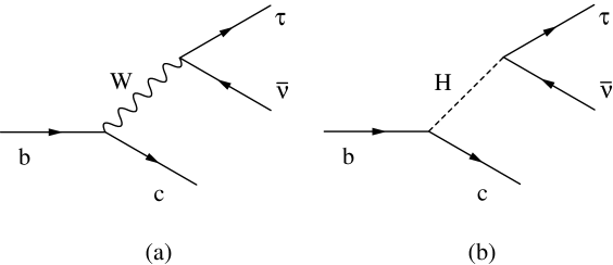
FIG. 1.: Quark-level diagrams for the transition $b\to c\tau\overline{\nu}$ in a two-Higgs doublet model.

=100pt

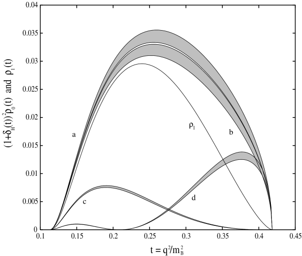
FIG. 2.: Spin-0 and spin-1 contributions to the differential distribution in the standard model and in two Higgs doublet models with various values of $\tan\beta/m_{H}$. The shaded bands labeled a, b, c and d correspond to the spin-0 contribution, $(1+\delta_{H}(t))^{2}\rho_{0}(t)$, with $\tan\beta/m_{H}=0$ (the SM), $0.06$ GeV^-1, $0.25$ GeV^-1 and $0.35$ GeV^-1, respectively. The solid curve corresponds to the spin-1 contribution, $\rho_{1}(t)$. The shaded regions indicate the current theoretical uncertainty in $(1+\delta_{H}(t))^{2}\rho_{0}(t)$ (due to the uncertainty in $\zeta(t)=F_{0}(t)/F_{1}(t)$) if $\rho_{1}(t)$ is known exactly. Uncertainties in $F_{S}(t)$ have not been included in this plot.

=100pt

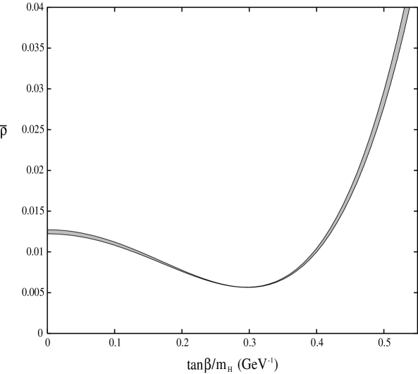
FIG. 3.: Plot of the integrated width (normalized to $G_{F}^{2}|V_{cb}|^{2}m_{B}^{5}/128\pi^{3}$) as a function of $\tan\beta/m_{H}$. As in Fig. 2, the shaded region corresponds to the theoretical uncertainty in $\zeta(t)=F_{0}(t)/F_{1}(t)$ and does not take into account the uncertainty in the scalar form factor, $F_{S}(t)$.

=100pt

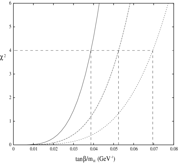
FIG. 4.: $\chi^{2}$ for the optimized weighting technique as a function of $\tan\beta/m_{H}$. The “input model” in this case is the standard model (i.e., $\tan\beta/m_{H}$$=$$0$). The solid, dashed and short-dashed curves correspond to $10^{4}$, $3\times 10^{3}$ and $10^{3}$ events, respectively. The vertical dashed lines indicate the $2\sigma$ upper bound on $\tan\beta/m_{H}$ in each case, with the regions to the right of the dashed lines being excluded.

=100pt

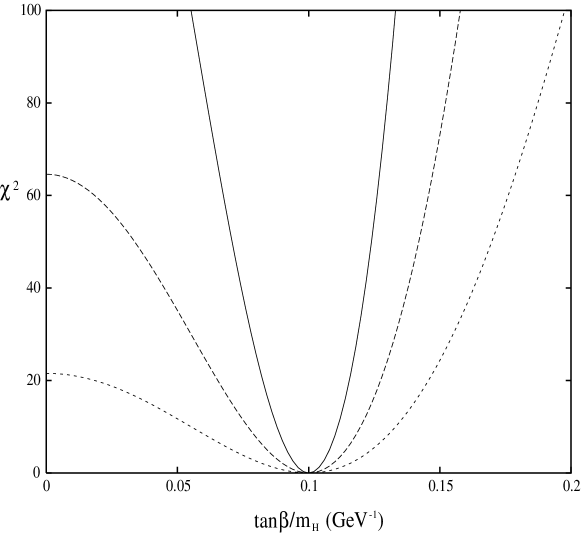
FIG. 5.: $\chi^{2}$ for the optimized weighting technique as a function of $\tan\beta/m_{H}$ in a two Higgs doublet model. The “input model” in this case has $\tan\beta/m_{H}=0.1$ GeV^-1. The solid, dashed and short-dashed curves correspond to $10^{4}$, $3\times 10^{3}$ and $10^{3}$ events, respectively. The intercept at $\tan\beta/m_{H}=0$ shows that for $10^{3}$ events one can distinguish this scenario from the standard model at approximately the $4.6\sigma$ level.