Abstract
We update our previous work on an analysis of the electroweak data by including new and partly preliminary data available up to the 1996 summer conferences. The new results on the $Z$ partial decay widths into $b$ and $c$ hadrons now offer a consistent interpretation of all data in the minimal standard model. The value extracted for the strong interaction coupling constant $\alpha_{s}(m_{Z})$ agrees well with determinations in other areas. New constraints on the universal parameters $S$, $T$ and $U$ are obtained from the updated measurements. No signal of new physics is found in the $S$, $T$, $U$ analysis once the SM contributions with $m_{t}\sim 175$GeV and those of not a too heavy Higgs boson are accounted for. The naive QCD-like technicolor model is now ruled out at the 99%CL even for the minimal model with ${\rm SU(2)_{TC}}$. In the absence of a significant new physics effect in the electroweak observables, constraints on masses of the top quark, $m_{t}$, and Higgs boson, $m_{H}$, are derived as a function of $\alpha_{s}$ and the QED effective coupling $\bar{\alpha}(m_{Z}^{2})$. The preferred range of $m_{H}$ depends rather strongly on the actual value of $m_{t}$ : $m_{H}<360{\,\rm GeV}$ for $m_{t}=170{\,\rm GeV}$, while $m_{H}>130{\,\rm GeV}$ for $m_{t}=180{\,\rm GeV}$ at 95 %CL. Prospects due to forthcoming improved measurements of asymmetries, the mass of the weak boson $W$ $m_{W}$, $m_{t}$ and $\bar{\alpha}(m_{Z}^{2})$ are discussed. Anticipating uncertainties of 0.00020 for $\bar{s}^{2}(m_{Z}^{2})$, 20 MeV for $m_{W}$, and 2 GeV for $m_{t}$, the new physics contributions to the $S$, $T$, $U$ parameters will be constrained more severely, and, within the SM, the logarithm of the Higgs mass can be constrained to about $\pm 0.35$. The better constraints on $S$, $T$, $U$ and on $m_{H}$ within the minimal SM should be accompanied with matching precision in $\bar{\alpha}(m_{Z}^{2})$.

To be published in Zeitshrift für Physik C

1 Introduction

The physics program of LEP1 is completed and has brought a wealth of precise data at the $Z$-resonance. With the presentation of the updated measurements at the 1996 summer conferences[1] an appropriate moment has come to assess the impact of the new data in the context of the theoretical framework introduced in Refs.[2, 3].

The $Z$-shape variables are now quite well measured (see Table 1), also the apparent discrepancy of the previous $R_{b}$ and $R_{c}$ measurements[4] with their Standard Model (SM) expectations seems to be solved. After combining the preliminary data from all LEP experiments and from SLD, the $R_{c}$ value is now in good agreement with the SM, while $R_{b}$ is less than 2 standard deviations away from the SM prediction. These new measurements are of importance when extracting a reliable value for the QCD coupling constant $\alpha_{s}(m_{Z})$ from the electroweak data.

The paper is organized as follows. In section 2 all electroweak measurements from LEP, SLC and Tevatron reported to the Warsaw Conference[1], are collected. These data are compared with the SM predictions[2] and a few remarkable features are pointed out. In section 3 a brief review is given of the electroweak radiative corrections in generic $\rm{SU(2)_{L}\times U(1)_{Y}}$ models following the formalism of Ref.[2]. In section 4 the impact of the new measurements is discussed, in particular the $Z$-shape parameter measurements at LEP/SLC and the new neutrino measurement of CCFR. A comprehensive fit to all the electroweak data is performed in terms of the three parameters[5] $S$, $T$, $U$, which characterize possible new physics contributions through the electroweak gauge-boson propagator corrections, and $\bar{\delta}_{b}$ which characterizes possible new physics contributions to the $Zb_{L}b_{L}$ vertex. Section 5 is devoted to the interpretation of all electroweak data within the minimal SM. Their constraints are shown as functions of $\alpha_{s}(m_{Z})$ and $\bar{\alpha}(m_{Z}^{2})$ in the $(m_{t},m_{H})$-plane. A brief discussion on the significance of bosonic radiative corrections containing the weak boson self-couplings is also given. In section 6 the impact of future improved measurements of the $Z$ boson asymmetries, the $W$ and top-quark masses and $\bar{\alpha}(m_{Z}^{2})$ are studied. Finally, section 7 gives a summary and outlook.

2 Electroweak Precision Data

Since our first analysis of electroweak data[2] a considerable improvement occurred in three areas, which is summarized in Table 1. The LEP Electroweak Working Group[1] has updated their results by including their preliminary electroweak data available up to summer 1996. The table contains also the results from SLC[1] and new Tevatron data on the $W$ mass[6] and the neutrino neutral current experiment[7]. Correlation matrices among the errors of the line-shape parameters and the heavy-quark parameters are given in Tables 2 and 3, respectively. All the numerical results presented in this paper are based on the unchanged data in Ref.[2] and the updated data in Tables 1–3, unless otherwise stated. Also shown in Table 1 are the SM predictions[2] for $m_{t}=175$ GeV, equal to the present best value from CDF and D0[8], $m_{H}=100$ GeV, $\alpha_{s}(m_{Z})=0.118$ and $1/\bar{\alpha}(m_{Z}^{2})=128.75$. The sensitivity of the fit results due to the uncertainties of the QCD and QED running coupling strengths will be discussed in sections 4, 5 and 6. The right-most column gives the difference between the mean of the data and the corresponding SM prediction in units of the experimental error. The data and the SM predictions agree fairly well. The previously[4] larger values of $R_{b}$ and smaller values of $R_{c}$ are now close to the SM prediction.

Table 1: Summary of new electroweak results since our first analysis[2]. These data represent the status as of the 1996 summer conferences and contain contributions from LEP and SLC[1] and Tevatron, $p\bar{p}$[6] and CCFR[7]. The SM predictions[2] are calculated for $m_{t}=175$ GeV, $m_{H}=100$ GeV, $\alpha_{s}(m_{Z})=0.118$, and $1/\bar{\alpha}(m_{Z}^{2})=128.75$; see section 3 for the definition of $\bar{\alpha}(m_{Z}^{2})$ and its uncertainty. Heavy flavor results are obtained by combining data from LEP and SLC[1].

		data	SM	${\rm\frac{\langle data\rangle-SM}{(error)}}$
LEP
	line shape:
	${m_{Z}}$(GeV)	$91.1863\pm 0.0020$	—	—
	${\Gamma_{Z}}$(GeV)	$2.4946\pm 0.0027$	$2.4972$	$-1.0$
	${\sigma_{h}^{0}}$(nb)	$41.508\pm 0.056$	$41.474$	$0.6$
	${R_{\ell}\equiv}\Gamma_{h/}\Gamma_{\ell}$	$20.778\pm 0.029$	$20.747$	$1.1$
	${A_{\rm FB}^{0,\ell}}$	$0.0174\pm 0.0010$	$0.0168$	$0.6$
	$\tau$ polarization:
	${A_{\tau}}$	$0.1401\pm 0.0067$	$0.1485$	$-1.3$
	${A_{e}}$	$0.1382\pm 0.0076$	$0.1486$	$-1.4$
	heavy flavor results:
	${R_{b}\equiv}\Gamma_{b/}\Gamma_{h}$	$0.2178\pm 0.0011$	$0.2157$	$1.9$
	${R_{c}\equiv}\Gamma_{c/}\Gamma_{h}$	$0.1715\pm 0.0056$	$0.1721$	$-0.1$
	${A_{\rm FB}^{0,b}}$	$0.0979\pm 0.0023$	$0.1041$	$-2.7$
	${A_{\rm FB}^{0,c}}$	$0.0735\pm 0.0048$	$0.0747$	$-0.2$
	jet charge asymmetry:
	$\sin^{2}\theta^{\rm lept}_{\rm eff}(\langle Q_{FB}\rangle)$	$0.2320\pm 0.0010$	$0.2313$	$0.7$
SLC
	${A_{LR}^{0}}$	$0.1542\pm 0.0037$	$0.1485$	$1.5$
	${A_{b}}$	$0.863\pm 0.049$	$0.935$	$-1.5$
	${A_{c}}$	$0.625\pm 0.084$	$0.668$	$-0.5$
Tevatron
$p\bar{p}$
	${m_{W}}$	$80.356\pm 0.125$	$80.400$	$-0.4$
CCFR
	$K$	$0.5626\pm 0.0060$	$0.5669$	$0.7$

Table 2: The error correlation matrix for the $Z$ line-shape parameters[1].

	$m_{Z}$	$\Gamma_{Z}$	$\sigma_{\rm h}^{0}$	$R_{\ell}$	$A_{\rm FB}^{0,\ell}$
$m_{Z}$	1.00	0.09	$-$0.01	$-$0.01	0.08
$\Gamma_{Z}$	0.09	1.00	$-$0.14	$-$0.01	0.00
$\sigma_{\rm h}^{0}$	$-$0.01	$-$0.14	1.00	0.15	0.01
$R_{\ell}$	$-$0.01	$-$0.01	0.15	1.00	0.01
$A_{\rm FB}^{0,\ell}$	0.08	0.00	0.01	0.01	1.00

Table 3: The error correlation matrix for the $b$ and $c$ quark results[1].

	$R_{b}$	$R_{c}$	$A_{\rm FB}^{0,b}$	$A_{\rm FB}^{0,c}$	$A_{b}$	$A_{c}$
$R_{b}$	1.00	$-$0.23	0.00	0.00	$-$0.03	0.01
$R_{c}$	$-$0.23	1.00	0.04	$-$0.06	0.05	$-$0.07
$A_{\rm FB}^{0,b}$	0.00	0.04	1.00	0.10	0.04	0.02
$A_{\rm FB}^{0,c}$	0.00	$-$0.06	0.10	1.00	0.01	0.10
$A_{b}$	$-$0.03	0.05	0.04	0.01	1.00	0.12
$A_{c}$	0.01	$-$0.07	0.02	0.10	0.12	1.00

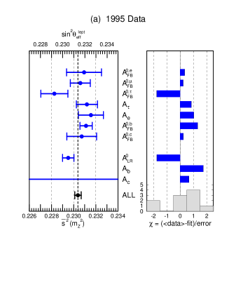
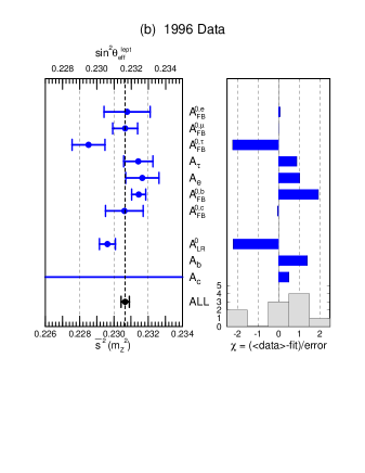
Figure 1: The effective electroweak mixing parameter ${\bar{s}}^{2}(m_{Z}^{2})$ is determined from the asymmetry data from LEP and SLC. The data up to 1995 and up to 1996 are displayed separately. The effective parameter $\sin^{2}\theta_{\rm eff}^{\rm lept}$ of the LEP Electroweak Working Group[4, 1] is related to ${\bar{s}}^{2}(m_{Z}^{2})$[2] by $\sin^{2}\theta_{\rm eff}^{\rm lept}\approx{\bar{s}}^{2}(m_{Z}^{2})+0.0010$. The $A_{b}$-measurement is off scale.

All the asymmetry data, including the left-right beam-polarization asymmetry, $A_{\rm LR}$, from SLC are compared in Fig. 1. It shows the result of a one-parameter fit to the asymmetry data in terms of the effective electroweak mixing angle, $\bar{s}^{2}(m_{Z}^{2})$[2]. In the SM (for details see sect.4) its numerical value is related to the effective parameter $\sin^{2}\theta_{\rm eff}^{\rm lept}$ adopted by the LEP group [4, 1] as follows : $\bar{s}^{2}(m_{Z}^{2})\approx\sin^{2}\theta_{\rm eff}^{\rm lept}-0.0010$[2]. The lepton forward-backward asymmetry is shown separately for each species. The fit to all 10 measurements yields :

$$\bar{s}^{2}(m_{Z}^{2})=0.23065\pm 0.00024$$ (2.1)

with $\chi^{2}_{\rm min}/({\rm d.o.f.})=17.3/(9)$. The updated measurements of the asymmetries barely agree (4%CL) with the hypothesis of being determined by a universal electroweak mixing parameter. The new fit is slightly worse than the corresponding one to the 1995 data[4] which gave[9] $\bar{s}^{2}(m_{Z}^{2})=0.23039\pm 0.00029$ with $\chi^{2}_{\rm min}/({\rm d.o.f.})=13.0/(9)$ or 16%CL.

In the analysis presented below we use the data of Table 1 and combine, assuming lepton ($e$–$\mu$–$\tau$) universality, the three forward-backward lepton asymmetries into the average forward-backward lepton asymmetry $A_{\rm FB}^{\ell,0}$ on the $Z$-pole. Using the data of Table 1 with $A_{\rm FB}^{\ell,0}$ instead of the three separate asymmetry measurements (see Fig. 1) one obtains :

$$\bar{s}^{2}(m_{Z}^{2})=0.23064\pm 0.00025$$ (2.2)

with $\chi^{2}_{\rm min}/({\rm d.o.f})=14.1/(7)$. Both the value and the probability of the fit (5%CL) remain nearly unchanged compared to (2.1). The somewhat low probability of the fits reflects the fact that two of the most accurate measurements, $A_{\rm LR}^{0}$ and $A_{\rm FB}^{b,0}$, are about two standard deviations from the mean to opposite sides as seen in Fig. 1. For instance, ignoring all hadron jet asymmetries and performing the fit with the lepton asymmetry data alone ($A_{\rm FB}^{\ell,0},\,A_{\tau},\,A_{e}\,A_{\rm LR}^{0}$) one obtains

$$\bar{s}^{2}(m_{Z}^{2})=0.23019\pm 0.00031$$ (2.3)

with $\chi^{2}/({\rm d.o.f})=6.0/(3)$. The fitted mean value decreases by about two standard deviations and the probability of the fit improves to 11%CL.

The quantity $K$ in Table 1 is a new measurement[7] obtained by the CCFR Collaboration from their neutrino data.

The value of the $W$-mass has been slightly improved[6].

3 Theoretical framework — Brief Review of Electroweak Radiative Corrections in $\rm{SU(2)_{L}\times U(1)_{Y}}$ Models

The formalism introduced in Ref.[2] is used to interpret the electroweak data. We use only those electroweak data that are most model independent, such as those listed in Table 1 of this report and those in Table 6 of Ref.[2]. We then express them in terms of the $S$-matrix elements of the processes with external quarks and leptons (with or without external QED and QCD corrections, depending on how the electroweak data are evaluated by experiments). These $S$-matrix elements are then evaluated in a generic $\rm SU(2)\times U(1)$ model with four charge form factors, $\bar{e}^{2}(q^{2})$, $\bar{s}^{2}(q^{2})$, $\bar{g}_{Z}^{2}(q^{2})$ and $\bar{g}_{W}^{2}(q^{2})$. An additional parameter $\mbox{$\bar{\delta}_{b}$}(m_{Z}^{2})$ related to the $Zb_{L}b_{L}$ vertex form factor is also introduced. By assuming negligible new physics contribution to the remaining vertex and box corrections, we derive constraints on the $4+1$ form factors from the model-independent data. By further assuming negligible new physics contribution to the running of the charge form factors, we derive constraints on $S$, $T$, $U$ and $\mbox{$\bar{\delta}_{b}$}(m_{Z}^{2})$. Finally, by assuming no new physics contribution at all, we can constrain $m_{t}$ and $m_{H}$. In this section a brief review of the salient features are given.

The propagator corrections in generic $\rm{SU(2)_{L}\times U(1)_{Y}}$ models can be conveniently expressed in terms of the following four effective charge form factors[2]:

(3.4a)

(3.4b)

(3.4c)

(3.4d)

where $\overline{\Pi}_{T,V}^{AB}(q^{2})\equiv[\overline{\Pi}_{T}^{AB}(q^{2})\!-\!\overline{\Pi}_{T}^{AB}(m_{V}^{2})]/(q^{2}\!-\!m_{V}^{2})$ are the propagator correction factors that appear in the $S$-matrix elements after the weak boson mass renormalization is performed, and $\hat{e}\equiv\hat{g}\hat{s}\equiv\hat{g}_{Z}\hat{s}\hat{c}$ are the $\overline{\rm MS}$ couplings. The ‘overlines’ denote the inclusion of the pinch terms[10, 11], which make these effective charges useful[12, 2, 13, 14] even at very high energies ($|q^{2}|\gg m_{Z}^{2}$). The amplitudes are then expressed in terms of these charge form factors plus appropriate vertex and box corrections. In our analysis[2] we assumed that all the vertex and box corrections are dominated by the SM contributions, except for the $Zb_{L}b_{L}$ vertex,

$$\Gamma_{L}^{Zbb}(q^{2})=-\hat{g}_{Z}\Bigl{\{}-\frac{1}{2}[1+\mbox{$\bar{\delta}_{b}$}(q^{2})]+\frac{1}{3}\hat{s}^{2}[1+\Gamma_{1}^{b_{L}}(q^{2})]\Bigr{\}},$$ (3.5)

for which the function $\mbox{$\bar{\delta}_{b}$}(m_{Z}^{2})$ is allowed to take on an arbitrary value. Hence the charge form factors and $\bar{\delta}_{b}$ can be directly extracted from the experimental data and their values be compared with the theoretical predictions.

We define[2] the $S$, $T$, and $U$ variables of Ref.[5] in terms the effective charges,

$$\frac{\bar{s}^{2}(m_{Z}^{2})\bar{c}^{2}(m_{Z}^{2})}{\bar{\alpha}(m_{Z}^{2})}-\frac{4\,\pi}{\bar{g}_{Z}^{2}(0)} \equiv \;\frac{S}{4}\,,$$ (3.6a)

$$\frac{\bar{s}^{2}(m_{Z}^{2})}{\bar{\alpha}(m_{Z}^{2})}\quad-\frac{4\,\pi}{\bar{g}_{W}^{2}(0)} \equiv \frac{S+U}{4}\,,$$ (3.6b)

$$1\;-\,\frac{\bar{g}_{W}^{2}(0)}{m_{W}^{2}}\frac{m_{Z}^{2}}{\bar{g}_{Z}^{2}(0)} \equiv \;\alpha T\,,$$ (3.6c)

where it is made manifest that these variables measure deviations from the tree-level universality of the electroweak gauge boson couplings. Here $\bar{c}^{2}=1-\bar{s}^{2}$ and $\bar{\alpha}(q^{2})=\bar{e}^{2}(q^{2})/4\pi$. They receive contributions from both the SM radiative effects and new physics contributions. The $S$, $T$, $U$ variables[5] as introduced by Peskin and Takeuchi are obtained[2] approximately by subtracting the SM contributions (at $m_{H}=1000$ GeV).

For a given electroweak model we can calculate the $S$, $T$, $U$ parameters ($T$ is a free parameter in models without the custodial SU(2) symmetry), and the charge form factors are then fixed by the following identities[2]:

$$\frac{1}{\bar{g}_{Z}^{2}(0)} = \frac{1+\bar{\delta}_{G}-\alpha\,T}{4\,\sqrt{2}\,G_{F}\,m_{Z}^{2}}\,,$$ (3.7a)

$$\bar{s}^{2}(m_{Z}^{2}) = \frac{1}{2}-\sqrt{\frac{1}{4}-\bar{\alpha}(m_{Z}^{2})\biggl{(}\frac{4\,\pi}{\bar{g}_{Z}^{2}(0)}+\frac{S}{4}\biggr{)}}\,,$$ (3.7b)

$$\frac{4\,\pi}{\bar{g}_{W}^{2}(0)} = \frac{\bar{s}^{2}(m_{Z}^{2})}{\bar{\alpha}^{2}(m_{Z}^{2})}-\frac{1}{4}\,(S+U)\,.$$ (3.7c)

Here $\bar{\delta}_{G}$ is the vertex and box correction to the muon lifetime[15] after subtracting the pinch term[2]:

$$G_{F} = \frac{\bar{g}_{W}^{2}(0)+\hat{g}^{2}\bar{\delta}_{G}}{4\,\sqrt{2}m_{W}^{2}}\,.$$ (3.8)

In the SM, $\bar{\delta}_{G}=0.0055$[2].

It is clear from the above identities that once we know $T$ and $\bar{\delta}_{G}$ in a given model we can predict $\bar{g}_{Z}^{2}(0)$, and then with the knowledge of $S$ and $\bar{\alpha}(m_{Z}^{2})$ we can calculate $\bar{s}^{2}(m_{Z}^{2})$, and with the further knowledge of $U$ we can calculate $\bar{g}_{W}^{2}(0)$. Since $\bar{\alpha}(0)=\alpha$ is known precisely, all four charge form factors are fixed at one $q^{2}$ point. The $q^{2}$-dependence of the form factors can also be calculated in a given model, but it is less dependent on physics at very high energies[2]. In the following analysis we assume that the SM contribution governs the running of the charge form factors between $q^{2}=0$ and $q^{2}=m_{Z}^{2}$. We can then predict all the neutral-current amplitudes in terms of $S$ and $T$, and the additional knowledge of $U$ gives the $W$ mass via Eq. (3.8).

We should note here that our prediction for the effective mixing parameter $\bar{s}^{2}(m_{Z}^{2})$ is not only sensitive to the $S$ and $T$ parameters but also on the precise value of $\bar{\alpha}(m_{Z}^{2})$. This is the reason why our predictions for the asymmetries measured at LEP/SLC and, consequently, the experimental constraint on $S$ extracted from the asymmetry data are sensitive to $\bar{\alpha}(m_{Z}^{2})$. In order to keep track of the uncertainty associated with $\bar{\alpha}(m_{Z}^{2})$ the parameter $\delta_{\alpha}$ was introduced in Ref.[2] as follows: $1/\bar{\alpha}(m_{Z}^{2})\!\equiv\!4\pi/\bar{e}(m_{Z}^{2})\!=\!128.72\!+\!\delta_{\alpha}$. We show in Table 4 the results of the four most recent updates[16, 17, 18, 19] on the hadronic contribution to the running of the effective QED coupling. Three definitions of the running QED coupling are compared. The effective charge $\bar{\alpha}(m_{Z}^{2})$ should be used in Eqs.(3) and (3), since the effective charges in (3) contain both fermionic and bosonic contributions to the gauge boson propagator corrections.

Table 4: The running QED coupling at the $m_{Z}$ scale in the three schemes. $1/\alpha(m_{Z}^{2})_{\rm l.f.}$ contains only the light fermion contributions to the running of the QED coupling constant between $q^{2}=0$ and $q^{2}=m_{Z}^{2}$. $1/\alpha(m_{Z}^{2})_{\rm f}$ contains all fermion contributions including the top-quark. The values $m_{t}=175$ GeV and $\alpha_{s}(m_{Z})=0.12$ in the perturbative two-loop correction[20] are assumed. $1/\bar{\alpha}(m_{Z}^{2})$ contains also the $W$-boson-loop contribution[2] including the pinch term[10, 11].

	$1/\alpha(m_{Z}^{2})_{\rm l.f.}$	$1/\alpha(m_{Z}^{2})_{\rm f}$	$1/\bar{\alpha}(m_{Z}^{2})$	$\delta_{\alpha}$
Martin-Zeppenfeld ’94[16]	$128.98\pm 0.06$	$128.99\pm 0.06$	$128.84\pm 0.06$	$0.12\pm 0.06$
Swartz ’95[17]	$128.96\pm 0.06$	$128.97\pm 0.06$	$128.82\pm 0.06$	$0.10\pm 0.06$
Eidelman-Jegerlehner ’95[18]	$128.89\pm 0.09$	$128.90\pm 0.09$	$128.75\pm 0.09$	$0.03\pm 0.09$
Burkhardt-Pietrzyk ’95[19]	$128.89\pm 0.10$	$128.90\pm 0.10$	$128.76\pm 0.10$	$0.04\pm 0.10$

Figure 2: Various estimates of $\Delta\alpha_{\rm had}(m_{Z}^{2})$ and the resulting $\bar{\alpha}(m_{Z}^{2})$ in the minimal SM. The parameter $\delta_{\alpha}$[2] is defined as $\delta_{\alpha}\equiv 1/\bar{\alpha}(m_{Z}^{2})-128.72$.

The new and some earlier estimates[21, 22, 23] are also shown in Fig. 2. The analysis of Ref.[2] was based on the estimate [23], $\delta_{\alpha}=0.00\pm 0.10$. The last four estimates made use of essentially the same total cross section data set for the process $\mbox{$e^{+}e^{-}$}\rightarrow{\rm hadrons}$ between the two-pion threshold and the $Z$ mass scale. The estimates are slightly different reflecting different procedures adopted by each group to interpolate between the available data points. Eidelman and Jegerlehner [18] and Burkhardt and Pietrzyk[19] made no assumption on the shape ($s$-dependence) of the cross section, and hence their errors are conservative. Swartz[17] assumed smoothness of $s$-dependence of the cross section in order to profit from the smaller point-to-point errors within each experiment. Martin and Zeppenfeld[16] also made use of the smaller experimental point-to-point errors by constraining the overall normalization on the basis of the perturbative QCD prediction with $\alpha_{s}(m_{Z})=0.118\pm 0.007$ down to $\sqrt{s}=3$ GeV. The smaller errors of these two estimates are obtained either because of the data point with the smallest normalization error[17] or because of replacing the large normalization uncertainty by the small uncertainty of the perturbative QCD prediction[16] in the region 3 GeV$<\sqrt{s}<7$ GeV. The mean values of the two estimates[16, 17] are similar as a result of the fact that the measured cross section of the smallest normalization error in the above region agrees roughly with the perturbative QCD prediction. In the following analysis we adopt as a standard the conservative estimate of Ref.[18], i.e. $\delta_{\alpha}=0.03\pm 0.09$ and investigate the sensitivity of our results to the deviation $\delta_{\alpha}-0.03$. We also show results of the analysis when the estimate[16] $\delta_{\alpha}=0.12\pm 0.06$ is adopted instead.

Once $\bar{\alpha}(m_{Z}^{2})$ is fixed the charge form factors in Eq. (3) can be calculated from $S$, $T$, $U$. The following approximate formulae[2] are useful:

$$\bar{g}_{Z}^{2}(0) \approx 0.5456\hphantom{+0.0036\,S^{\prime}}\;\,+0.0040\,T^{\prime}\,,$$ (3.9a)

$$\bar{s}^{2}(m_{Z}^{2}) \approx 0.2334+0.0036\,S^{\prime}-0.0024\,T^{\prime}\,\,,\qquad$$ (3.9b)

$$\bar{g}_{W}^{2}(0) \approx 0.4183-0.0030\,S^{\prime}+0.0044\,T^{\prime}+0.0035\,U^{\prime}\,\,,\qquad$$ (3.9c)

where

$$S^{\prime} = S-0.72\,\delta_{\alpha}\,,$$ (3.10a)

$$T^{\prime} = T+(0.0055-\bar{\delta}_{G})/\alpha\,,$$ (3.10b)

$$U^{\prime} = U-0.22\,\delta_{\alpha}\,.$$ (3.10c)

The values of $\bar{g}_{Z}^{2}(m_{Z}^{2})$ and $\bar{s}^{2}(0)$ are then calculated from $\bar{g}_{Z}^{2}(0)$ and $\bar{s}^{2}(m_{Z}^{2})$ above, respectively, by assuming the SM running of the form factors. The $Z$ widths are sensitive to $\bar{g}_{Z}^{2}(m_{Z}^{2})$, which can be obtained from $\bar{g}_{Z}^{2}(0)$ in the SM approximately by

$$\frac{4\pi}{\bar{g}_{Z}^{2}(m_{Z}^{2})}\approx\frac{4\pi}{\bar{g}_{Z}^{2}(0)}-0.299+0.031\log\biggl{[}1+\Bigl{(}\frac{26{\rm GeV}}{m_{H}}\Bigr{)}^{2}\biggr{]}.$$ (3.11)

The approximation is valid to 0.001 provided $m_{t}>160{\,\rm GeV}$ and $m_{H}>40{\,\rm GeV}$. On the other hand the low energy neutral current experiments are sensitive to $\bar{s}^{2}(0)$ which is obtained by assuming the SM running of the charge form factor $\bar{s}^{2}(q^{2})/\bar{\alpha}(q^{2})$:

$$\frac{\bar{s}^{2}(0)}{\alpha}\approx\frac{\bar{s}^{2}(m_{Z}^{2})}{\bar{\alpha}(m_{Z}^{2})}+3.09-\frac{\delta_{\alpha}}{2}.$$ (3.12)

Finally, within the SM the $S$, $T$, $U$ parameters and the form factor $\mbox{$\bar{\delta}_{b}$}=\bar{\delta}_{b}(m_{Z}^{2})$ are functions of $m_{t}$ and $m_{H}$ which can be parametrized as

$$S_{\rm SM} \approx -0.233-0.007\mbox{$x_{t}$}+0.091\mbox{$x_{H}$}-0.010x_{H}^{2}\,,$$ (3.13a)

$$T_{\rm SM} \approx +0.879+(0.130-0.003\mbox{$x_{H}$})\mbox{$x_{t}$}+0.003\mbox{$x_{t}$}^{2}-0.079\mbox{$x_{H}$}-0.028x_{H}^{2}+0.0026x_{H}^{3}\,,$$

$$U_{\rm SM} \approx +0.362+0.022\mbox{$x_{t}$}-0.002\mbox{$x_{H}$}\,,$$ (3.13c)

$$\mbox{$\bar{\delta}_{b}$}_{\rm SM} \approx -0.00995-0.00087\mbox{$x_{t}$}-0.00002\mbox{$x_{t}$}^{2}\,,$$ (3.13d)

where $\mbox{$x_{t}$}=(m_{t}({\,\rm GeV})-175)/10$ and $\mbox{$x_{H}$}=\log(m_{H}({\,\rm GeV})/100)$. The above approximate expressions are valid to $\pm 0.003$ for $S_{\rm SM}$, $T_{\rm SM}$ and $U_{\rm SM}$, and to $\pm 0.00007$ for $\mbox{$\bar{\delta}_{b}$}_{\rm SM}$ in the domain $160~{}{\,\rm GeV}<m_{t}<185~{}{\,\rm GeV}$ and $40~{}{\,\rm GeV}<m_{H}<1000~{}{\,\rm GeV}$. They are evaluated after all the two-loop corrections included in Ref.[2] are taken into account, for $\alpha_{s}(m_{Z})=0.118$ in the two-loop ${\cal O}(\alpha_{s})$ terms[20]. The $m_{H}$-dependence of the $\mbox{$\bar{\delta}_{b}$}(m_{Z}^{2})_{\rm SM}$ function is found to be negligibly small for the above region of $m_{t}$.

Note : Since the publication of our original paper[2] several improvements have been achieved on the SM radiative corrections. Most notably, we now have the three-loop (order $\alpha_{s}^{2}$) QCD calculation of the $T$ parameter[24] as well as in the gauge boson propagator corrections [25]. These three-loop effects slightly modify the relationship between the electroweak $S$, $T$, $U$ parameters and the physical top quark mass $m_{t}$ in the above formulae (2). After the completion of the present report we took note of the new evaluation of non-factorizable QCD and electroweak corrections to the hadronic $Z$ boson decay rates[26]. A negative correction to the $Z$ hadronic width was found reducing the SM prediction for $\Gamma_{h}$ by 0.59 MeV after summing over the four light quark flavors. The corresponding effect for the partial width $\Gamma(Z\rightarrow`b\bar{b}\mbox{'})$ has not been evaluated. This shift would in turn enhance the $\alpha_{s}$ value extracted from the electroweak data by 0.001. We refrain from modifying the numbers in the present report. If we assume that the corrections to the partial width $\Gamma(Z\rightarrow`b\bar{b}\mbox{'})$ is small, the net effect for the numbers due to the above new calculations would be as follows :

• The three-loop corrections to the $T$ parameter[24] modifies the relationship (LABEL:t_approx) between $T$ and the physical top quark mass. By comparing[24] with [2], we find

  $$\Bigl{[}m_{t}^{\rm(2-loop)}\Bigr{]}^{2}\Bigl{\{}1-\frac{2(3+\pi^{2})}{9}\frac{\alpha_{s}(m_{Z})}{\pi}\Bigr{\}}$$

  $$\quad=\Bigl{[}m_{t}^{\rm(3-loop)}\Bigr{]}^{2}\biggl{\{}1-\frac{2(3+\pi^{2})}{9}\frac{\alpha_{s}(m_{t})}{\pi}-14.594\Bigl{(}\frac{\alpha_{s}(m_{t})}{\pi}\Bigr{)}^{2}\biggr{\}}\,.$$ (3.14)

  This can be approximated as

  $$m_{t}^{\rm(2-loop)}=m_{t}^{\rm(3-loop)}\biggl{\{}1-(7.3-5.5\log\frac{m_{t}}{m_{Z}})\Bigl{(}\frac{\alpha_{s}(m_{Z})}{\pi}\Bigr{)}^{2}\biggr{\}}\,.$$ (3.15)

  For $m_{t}\sim 170{\,\rm GeV}$, this corresponds to the replacement of $m_{t}^{\rm(2-loop)}$ by $m_{t}^{\rm(3-loop)}-1{\,\rm GeV}$. Non-leading three-loop corrections calculated in [25] modifies $S_{\rm SM}$, $U_{\rm SM}$ in (2) and the running of the $\bar{g}_{Z}^{2}(q^{2})$ charge (3.11). Their effects are, however, much smaller than the leading effect as quoted above. Consequently, the three-loop ${\cal O}(\alpha_{s}^{2})$ effects can be approximately taken into account by replacing all the $m_{t}$ symbols in this report by the r.h.s. combination of Eq. (3.15), or roughly by $m_{t}-1{\,\rm GeV}$. In other words, the fitted $m_{t}$ value should be about $1{\,\rm GeV}$ larger, while the results with an external $m_{t}$ constraint should correspond to those where the external $m_{t}$ is increased by about $1{\,\rm GeV}$.

• The mixed QCD electroweak two-loop corrections of Ref.[26] can be accounted for by replacing all $\alpha_{s}$ symbols in this report by $\alpha_{s}-0.001$. In other words, the fitted $\alpha_{s}$ value should be about $0.001$ larger, while the results with an external $\alpha_{s}$ constraint should correspond to those where the external $\alpha_{s}$ is increased by about $0.001$. This is because the $\alpha_{s}$ dependences in the corrections other than the hadronic width of the $Z$ are all negligibly small.

4 Implications of the New Measurements

In this section the new results and their implications are discussed. Also a fit in terms of the $S$, $T$, $U$ parameters[5] of the electroweak gauge boson propagator corrections as well as of the $Zb_{L}b_{L}$ vertex form factor, $\mbox{$\bar{\delta}_{b}$}(m_{Z}^{2})$ is presented. The strengths of the QCD and QED couplings at the $m_{Z}$ scale, $\alpha_{s}(m_{Z})$ and $\bar{\alpha}(m_{Z}^{2})$, are treated as external parameters in the fits, so that implications of their precise knowledge affecting the fit results are made explicit.

4.1 New LEP/SLC data

The updated $Z$ shape parameter measurements (see Tables 1–3) are used to extract the charge form factors. It is assumed that the vertex corrections except for the $Zb_{L}b_{L}$ vertex function $\mbox{$\bar{\delta}_{b}$}(m_{Z}^{2})$ are dominated by the SM contributions. The free parameters are : $\bar{g}_{Z}^{2}(m_{Z}^{2})$, $\bar{s}^{2}(m_{Z}^{2})$, $\alpha_{s}^{\prime}$ and $\mbox{$\bar{\delta}_{b}$}(m_{Z}^{2})$. The quantity $\alpha_{s}^{\prime}$ is the combination

$$\alpha_{s}^{\prime}=\alpha_{s}(m_{Z})_{\overline{\rm MS}}\,+1.54\,[\mbox{$\bar{\delta}_{b}$}(m_{Z}^{2})+0.00995]$$ (4.16)

that appears[2, 3] in the theoretical prediction for $\Gamma_{h}$. The fit yields:

$$\!\!\left.\begin{array}[]{c@{\,}r@{\,}r@{\,}r@{\,}r}\bar{g}_{Z}^{2}(m_{Z}^{2})&=&0.55557&\pm&0.00074\\[2.84526pt] \bar{s}^{2}(m_{Z}^{2})&=&0.23065&\pm&0.00025\\[2.84526pt] \alpha_{s}^{\prime}&=&0.1218&\pm&0.0038\\[2.84526pt] \mbox{$\bar{\delta}_{b}$}(m_{Z}^{2})&=&-0.0051&\pm&0.0028\end{array}\right\}\;\rho_{\rm corr}=\left(\begin{array}[]{rrrr}1.00&0.13&-0.57&0.00\\[2.84526pt] &1.00&0.11&0.05\\[2.84526pt] &&1.00&0.01\\[2.84526pt] &&&1.00\\[2.84526pt] \end{array}\right),\,\,\,\qquad$$ (4.17i)

$$\chi^{2}_{\rm min}/({\rm d.o.f.})=15.4/(9)\,.$$ (4.17j)

The value of $\chi^{2}_{\rm min}$ is dominated by the contribution of the asymmetries which accounts for $14.1$ (cf. Eq. (2.2)). When allowing only $\bar{s}^{2}(m_{Z}^{2})$ and $\bar{g}_{Z}^{2}(m_{Z}^{2})$ to be fitted freely, and treating $\alpha_{s}^{\prime}$ and $\mbox{$\bar{\delta}_{b}$}(m_{Z}^{2})$ as external parameters, we obtain an equivalent result:

$$\left.\begin{array}[]{ll}\bar{g}_{Z}^{2}(m_{Z}^{2})&\!\!=0.55557-0.00042\,{\textstyle\frac{\alpha_{s}^{\prime}-0.1218}{0.0038}}\pm 0.00061\\[2.84526pt] \bar{s}^{2}(m_{Z}^{2})&\!\!=0.23065+0.00003\,{\textstyle\frac{\alpha_{s}^{\prime}-0.1218}{0.0038}}\pm 0.00024\end{array}\right\}\,\,\rho_{\rm corr}=0.24,$$ (4.18c)

$$\quad\chi^{2}_{\rm min}=15.4+\biggl{(}\frac{\alpha_{s}^{\prime}-0.1218}{0.0038}\biggr{)}^{2}+\biggl{(}\frac{\mbox{$\bar{\delta}_{b}$}+0.0051}{0.0028}\biggr{)}^{2}\,.$$ (4.18d)

Compared to the previous results in Ref.[2] the precision has increased by more than a factor of two.

The fit can be qualitatively understood as follows. The asymmetries determine almost exclusively $\bar{s}^{2}(m_{Z}^{2})$. The tiny difference between the above $\bar{s}^{2}(m_{Z}^{2})$ and Eq. (2.2) is due to the $\alpha_{s}^{\prime}$-dependence of $R_{\ell}$. The only quantity constraining $\bar{g}_{Z}^{2}(m_{Z}^{2})$ is $\Gamma_{Z}$ which also depends on $\bar{s}^{2}(m_{Z}^{2})$ and $\alpha_{s}^{\prime}$, thus explaining the non-negligible error correlations above. The quantity $\alpha_{s}^{\prime}$ is mainly determined by $R_{\ell}$ and also by $\sigma_{h}^{0}$. The observable $R_{b}$, i.e. the ratio of $\Gamma_{b}$ and $\Gamma_{h}$, is constraining $\mbox{$\bar{\delta}_{b}$}(m_{Z}^{2})$. It is interesting to note that the form factor $\mbox{$\bar{\delta}_{b}$}(m_{Z}^{2})$ is nearly uncorrelated from the other fit quantities because of our using the combination (4.16). It is now straightforward to obtain the best value of $\alpha_{s}$ from $\alpha_{s}^{\prime}$ and $\bar{\delta}_{b}$ :

$$\alpha_{s}=\alpha_{s}^{\prime}-1.54\,[\mbox{$\bar{\delta}_{b}$}+0.00995\,]=0.1143\pm 0.0057\,.$$ (4.19)

If on the other hand $R_{b}$ and $R_{c}$ are fixed to their SM predictions with $m_{t}=175$ GeV, i.e. $\mbox{$\bar{\delta}_{b}$}=-0.00995$, one obtains $\alpha_{s}=0.1218\pm 0.0038$. This little exercise demonstrates the crucial role of the $R_{b}$ and $R_{c}$ measurements in obtaining information on $\alpha_{s}$ from the precision $Z$ experiments.

Figure 3: The 1-sigma allowed contours in ($\bar{s}^{2}(m_{Z}^{2}),\bar{g}_{Z}^{2}(m_{Z}^{2})$) plane obtained from the fits to the $Z$ boson parameters. The solid contour is obtained by treating $\alpha_{s}^{\prime}$ and $\bar{\delta}_{b}$ as free parameters in the fit. Also shown are the results by treating $\alpha_{s}^{\prime}$ as an external parameter. Three values of $\alpha_{s}^{\prime}$ ($=0.115,0.118,0.121$), are chosen. The results are insensitive to the assumed $\bar{\delta}_{b}$ value. The grid illustrates the SM predictions in the range $140{\,\rm GeV}\!<\!m_{t}\!<\!200{\,\rm GeV}$ and $10{\,\rm GeV}\!<\!m_{H}\!<\!1000{\,\rm GeV}$ at $\delta_{\alpha}\!\equiv\!1/\bar{\alpha}(m_{Z}^{2})\!-\!128.72\!=\!0.03$, where their dependences on $\delta_{\alpha}\!-\!0.03$ are shown by a “$\longleftrightarrow$” symbol.

Figure 3 shows the fit result in the ($\bar{s}^{2}(m_{Z}^{2}),\bar{g}_{Z}^{2}(m_{Z}^{2})$) plane. The contours represent the 1-$\sigma$ (39%CL) allowed region. The solid contour shows the result of the four-parameter fit (4.1). Also shown are the results of the two-parameter fit in terms of $\bar{g}_{Z}^{2}(m_{Z}^{2})$ and $\bar{s}^{2}(m_{Z}^{2})$ treating $\alpha_{s}^{\prime}$ as an external parameter. Three values of $\alpha_{s}^{\prime}$ (0.115,0.118,0.121) are chosen in the figure, which correspond respectively to the $\alpha_{s}$ values in the SM at $m_{t}=175{\,\rm GeV}$; see (4.31d). The results are insensitive to the assumed $\bar{\delta}_{b}$ value once the magnitude of the combination $\alpha_{s}^{\prime}$ is fixed. The SM predictions for $\delta_{\alpha}=0.03$ and their dependence on $\delta_{\alpha}-0.03$ are also given. As expected from Eqs. (2), (3) and (2), only the predictions for $\bar{s}^{2}(m_{Z}^{2})$ is sensitive to $\delta_{\alpha}$.

4.2 The heavy quark sector and $\alpha_{s}$

The most striking results of the updated electroweak data are those of $R_{b}$ and $R_{c}$, which are shown in Fig. 4 juxtaposing the status as of summer 1995 and 1996. The SM predictions to these ratios are shown by the thick solid line, where the value of the top-quark mass affecting the $Zb_{L}b_{L}$ vertex correction is indicated by solid blobs. Although it was tempting to conclude from the 1995 data on $R_{b}$ and $R_{c}$ that the SM is excluded at 99.99%CL, it was also clear[9, 27] that it would be precocious to base such a far reaching conclusion on just these two measurements knowing how complex the analyses are and how critical the role of systematic effects is.

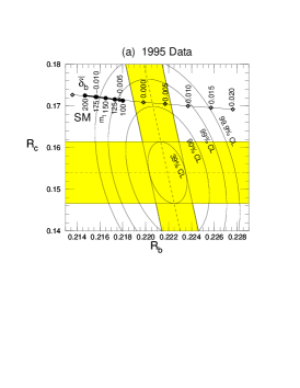
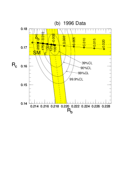
Figure 4: $R_{b}$ and $R_{c}$ data[4, 1] and the SM predictions[2].

It is useful to note the fact that the three most accurately measured line-shape parameters, $\Gamma_{Z}$, $\sigma_{h}^{0}$ and $R_{\ell}$ in Table 1, determine accurately the $Z$ partial widths $\Gamma_{l}$, $\Gamma_{h}$ and $\Gamma_{\rm inv}$, because they are three independent combinations of the three partial widths, i.e. $\Gamma_{Z}=\Gamma_{h}+3\Gamma_{l}+\Gamma_{\rm inv}$, $R_{l}=\Gamma_{h}/\Gamma_{l}$, and $\sigma_{h}^{0}=(12\pi/m_{Z}^{2})\Gamma_{h}\Gamma_{l}/\Gamma_{Z}^{2}$. We find

$$\begin{array}[]{c@{\;}c@{\;}l}\Delta\Gamma_{h}/(\Gamma_{h})_{\rm SM}&=&\phantom{-}0.0011\pm 0.0014\\ \Delta\Gamma_{l}/(\Gamma_{l})_{\rm SM}&=&-0.0013\pm 0.0013\\ \Delta\Gamma_{\rm inv}/(\Gamma_{\rm inv})_{\rm SM}&=&-0.0050\pm 0.0040\end{array}\quad\rho_{\rm corr}=\left(\begin{array}[]{rrr}1.00&0.49&-0.41\\ &1.00&0.23\\ &&1.00\end{array}\,\right)\,,$$ (4.26)

where $(\Gamma_{h})_{\rm SM}=1743.4{\,\rm MeV}$, $(\Gamma_{\ell})_{\rm SM}=84.03{\,\rm MeV}$ and $(\Gamma_{\rm inv})_{\rm SM}=501.9{\,\rm MeV}$ are the SM predictions[2] for $m_{t}=175{\,\rm GeV}$, $m_{H}=100{\,\rm GeV}$, $\alpha_{s}=0.118$ and $\mbox{$\delta_{\alpha}$}=0.03$. The high precision of 0.14% of the hadronic $Z$ partial width, $\Gamma_{h}$, strongly restricts any attempt to modify theoretical predictions for the ratios $R_{b}$ and $R_{c}$[9]. To see this, $\Gamma_{h}$ is approximately expressed as

$$\Gamma_{h} = \Gamma_{u}+\Gamma_{d}+\Gamma_{s}+\Gamma_{c}+\Gamma_{b}+\Gamma_{\rm others}$$ (4.27)

$$\sim \{\Gamma_{u}^{0}+\Gamma_{d}^{0}+\Gamma_{s}^{0}+\Gamma_{c}^{0}+\Gamma_{b}^{0}\}\times[1+\frac{\alpha_{s}}{\pi}+{\cal O}(\frac{\alpha_{s}}{\pi})^{2}],$$

where $\Gamma_{q}^{0}$’s are the partial widths in the absence of the final state QCD corrections. Hence, to a good approximation, the ratios $R_{q}$ can be expressed as ratios of $\Gamma_{q}^{0}$ and their sum. A decrease in $R_{b}$ and an increase in $R_{c}$ should then imply a decrease and an increase of $\Gamma_{b}^{0}$ and $\Gamma_{c}^{0}$, respectively, from their SM predicted values. The strong interaction coupling $\alpha_{s}$ acts like a flavor independent adjustment parameter. This is clearly borne out in Fig. 5, where, once both $\,\Gamma_{b}^{0}$ and $\Gamma_{c}^{0}$ are left free in the fit, the above $\Gamma_{h}$ drives $\alpha_{s}$ for the 1995 data[4] to an unacceptably large value, while for the 1996 update[1] a consistent picture emerges. On the other hand, if we allow only $\Gamma_{b}^{0}$ to vary by assuming the SM value of $\Gamma_{c}^{0}$ (the straight line of the extended SM in Fig. 4), then the $\Gamma_{h}$ constraint gives a slightly smaller value of $\alpha_{s}$, see Eq. (4.19), though still compatible with the global average[28], $\alpha_{s}=0.118\pm 0.003$.

Figure 5: $R_{b}+R_{c}$ vs $\alpha_{s}$. From the 1995 data[4](a) and the 1996 date[1](b).

In general, if we introduce a fractional change in the bare hadronic width

$$\frac{\delta\Gamma_{h}^{0}}{(\Gamma_{h}^{0})_{\rm SM}}\approx\frac{\sum_{q}\delta\Gamma_{q}^{0}}{\sum_{q}(\Gamma_{q}^{0})_{\rm SM}}\,,$$ (4.28)

one measures to a good approximation from the $Z$-line shape parameters the combination

$$\alpha_{s}+\pi\frac{\delta\Gamma_{h}^{0}}{(\Gamma_{h}^{0})_{\rm SM}}\,.$$ (4.29)

In other words, the effective parameter $\alpha_{s}^{\prime}$

$$\alpha_{s}^{\prime}\equiv\alpha_{s}(m_{Z})_{\overline{\rm MS}}+3.186\frac{\delta\Gamma_{h}^{0}}{(\Gamma_{h}^{0})_{\rm SM}}\,.$$ (4.30)

is constrained by the $Z$ parameters. The coefficient in front of the fractional width ratio is slightly larger than $\pi$ because of the higher-order QCD corrections. For definiteness, we use the SM prediction $(\Gamma_{h}^{0})_{\rm SM}=1678.7{\,\rm MeV}$ evaluated at $(m_{t},m_{H})=(175,100){\,\rm GeV}$. If only the $Zb_{L}b_{L}$ vertex is allowed to deviate from the SM prediction,

$$\alpha_{s}^{\prime} = \alpha_{s}+3.186\frac{\delta R_{b}}{1-R_{b}}$$ (4.31a)

$$\approx \alpha_{s}+1.54\Bigl{(}\mbox{$\bar{\delta}_{b}$}-[(\mbox{$\bar{\delta}_{b}$})_{\rm SM}]_{m_{t}=175{\,\rm GeV}}\Bigr{)}$$ (4.31b)

$$\approx \alpha_{s}+1.54(\mbox{$\bar{\delta}_{b}$}+0.00995)$$ (4.31c)

$$\approx \alpha_{s}+0.00134\mbox{$x_{t}$}+1.54\,[\mbox{$\bar{\delta}_{b}$}]_{\rm NewPhysics}$$ (4.31d)

in agreement with the expression (4.16). The last equality is obtained by inserting the SM expression (3.13d) for $\bar{\delta}_{b}$ where we neglect the small quadratic term. If both $R_{b}$ and $R_{c}$ are modified, it is the combination

$$\alpha_{s}^{\prime}=\alpha_{s}+3.186\frac{\delta R_{b}+\delta R_{c}}{1-R_{b}-R_{c}}$$ (4.32)

which is constrained by the $\Gamma_{h}$ data.

Figure 6: Constraint on $\alpha_{s}$ from the electroweak $Z$ boson data by assuming the SM for various $m_{t}$ and $m_{H}$ at $\mbox{$\delta_{\alpha}$}=0.03$. Also shown is the result of a more general fit, where $\Gamma_{b}$ is a free parameter. For comparison, the global average as obtained by the Particle Data Group[28] is shown.

At present, the LEP Collaborations have not yet completed their analyses of $R_{b}$ and $R_{c}$ by including the latest runs. However, there are new precise analyses of OPAL on $R_{c}$[29] and $R_{b}$[30] and one by ALEPH on $R_{b}$[31]. The new analyses aim at reducing as much as possible the use of information not directly obtainable from experiment itself. The increased number of tags in the ALEPH analysis implies also a smaller correlation between $R_{b}$ and $R_{c}$. The preliminary values quoted at the 1996 summer conferences[1] roughly agree with the SM expectation and it may now be meaningful to compare the constraints on the strong coupling constant $\alpha_{s}$ from the $Z$-pole data with those from other sectors [28] (see Fig. 6). We find the following parametrization for the $m_{t}$, $m_{H}$ and $\delta_{\alpha}$ dependences of the SM fit to $\alpha_{s}$:

$$\alpha_{s} = 0.1182\pm 0.0030-0.00075\mbox{$x_{t}$}+0.0023\mbox{$x_{H}$}+0.00046x_{H}^{2}-0.00074\mbox{$x_{\alpha}$}$$ (4.33)

where $\mbox{$x_{t}$}=(m_{t}({\,\rm GeV})-175)/10$, $\mbox{$x_{H}$}=\log(m_{H}({\,\rm GeV})/100)$, and $\mbox{$x_{\alpha}$}=(\mbox{$\delta_{\alpha}$}-0.03)/0.09$. The parametrization is valid in the range $150<m_{t}({\,\rm GeV})<200$, $60<m_{H}({\,\rm GeV})<1000$ and $|\delta_{\alpha}|<0.2$. It is remarkable that the electroweak data alone imply an intrinsic precision of $\pm 0.003$ (disregarding new physics contribution to the $Z$ partial widths) which is deteriorated by the imprecise knowledge of the external parameters, i.e. the masses of the top and Higgs and also by the running “QED” coupling $\alpha(m_{Z}^{2})$ (see also Section 5.1). It can be seen from Fig. 6 and the above parametrization that the agreement between the SM fit to the $Z$ parameters and the present world average of direct measurements, $\alpha_{s}=0.118\pm 0.003$, is good only for a relatively light Higgs boson ($m_{H}\hbox to0.0pt{\lower 3.5pt\hbox{$\mathchar 0\relax\sim$}\hss}\raise 1.0pt\hbox{$<$}300{\,\rm GeV}$).

4.3 New Neutrino Data

A new piece of information in the low-energy neutral current sector comes from the CCFR collaboration[7] which measured the neutral- to charged-current cross section ratio in $\nu_{\mu}$ scattering off nuclei. Using the model-independent parameters of Ref.[32], they constrain the following linear combination,

$$K = 1.732g_{L}^{2}+1.119g_{R}^{2}-0.100\delta_{L}^{2}-0.086\delta_{R}^{2}\,,$$ (4.34)

and obtain

$$K=0.5626\pm 0.0025\,\mbox{(stat)}\pm 0.0036\,\mbox{(sys)}\pm 0.0028\,\mbox{(model)}-0.0029\,\frac{m_{c}-1.31{\,\rm GeV}}{0.24{\,\rm GeV}},$$ (4.35)

with $m_{c}=(1.31\pm 0.24){\,\rm GeV}$. Because of the larger $\langle Q^{2}\rangle_{\rm CCFR}=36{{\,\rm GeV}}^{2}$ in the CCFR experiments compared to the old data[32] ($\langle Q^{2}\rangle_{\rm HF}=20{{\,\rm GeV}}^{2}$), the measurement is first expressed in terms of $\bar{s}^{2}(0)$ and $\bar{g}_{Z}^{2}(0)$ and then combined with the old data. Figure 7 shows the CCFR-band together with the ellipse of all previous $\nu q$-data.

Figure 7: Fit to the low-energy neutral-current data in terms of the two universal charge form factors $\bar{s}^{2}(m_{Z}^{2})$ and $\bar{g}_{Z}^{2}(m_{Z}^{2})$ which are calculated from $\bar{s}^{2}(0)$ and $\bar{g}_{Z}^{2}(0)$ by assuming the SM running of the charge form factors. 1-$\sigma$ (39%CL) contours are shown separately for the old[32] and the new[7] $\nu_{\mu}$–$q$ data, the $\nu_{\mu}$–$e$ data, the atomic parity violation (APV) data, and the SLAC $e$–${\rm D}$ polarization asymmetry data: see Ref.[2] The 1-$\sigma$ contour of the combined fit, Eq. (4.3), is shown by the thick ellipse. The little ellipse represents the 1-sigma constraint from LEP/SLC data corresponding to the solid ellipse of Fig. 3.

The CCFR data (4.35) being obtained after correcting for the external photonic corrections lead to the constraint :

$$\bar{s}^{2}(0)=0.2421+1.987[\bar{g}_{Z}^{2}(0)-0.5486]\pm 0.0058\,.$$ (4.36)

It should be noted that the old data[32] were also corrected for external photonic corrections. We find

$$\left.\begin{array}[]{ll}\bar{g}_{Z}^{2}(0)&=0.5454^{+0.0076}_{-0.0082}\\[2.84526pt] \bar{s}^{2}(0)&=0.2419^{+0.0130}_{-0.0142}\end{array}\right\}\quad\rho_{\rm corr}=0.916,$$ (4.37c)

$$\quad\chi^{2}_{\rm min}=0.13\,.$$ (4.37d)

The combination of the new CCFR data[7] with the previous neutrino data[32] yields:

$$\left.\begin{array}[]{ll}\bar{g}_{Z}^{2}(0)&=0.5476^{+0.0070}_{-0.0076}\\[2.84526pt] \bar{s}^{2}(0)&=0.2429^{+0.0128}_{-0.0140}\end{array}\right\}\quad\rho_{\rm corr}=0.955,$$ (4.38c)

$$\quad\chi^{2}_{\rm min}=0.7\quad({\rm d.o.f.}=3).$$ (4.38d)

The combined fit to all the low-energy neutral current data including those studied in Ref.[2] gives :

$$\left.\begin{array}[]{ll}\bar{g}_{Z}^{2}(0)&=0.5441\pm 0.0029\\[2.84526pt] \bar{s}^{2}(0)&=0.2362\pm 0.0044\end{array}\right\}\quad\rho_{\rm corr}=0.70,$$ (4.39c)

$$\quad\chi^{2}_{\rm min}=2.7\quad({\rm d.o.f.}=8)\,.$$ (4.39d)

For later convenience these results are also expressed at the shifted scale $q^{2}=m_{Z}^{2}$. Here we assume no significant new physics contributions to the running of the charge form factors from 0 to $m_{Z}^{2}$. Uncertainty from the $m_{H}$-dependence of the running of $\bar{g}_{Z}^{2}(m_{Z}^{2})$, Eq. (3.11), is negligibly small for $m_{H}>70{\,\rm GeV}$. The result is then :

$$\left.\begin{array}[]{ll}\bar{g}_{Z}^{2}(m_{Z}^{2})&=0.5512\pm 0.0030\\[2.84526pt] \bar{s}^{2}(m_{Z}^{2})&=0.2277\pm 0.0047\end{array}\right\}\quad\rho_{\rm corr}=0.70,$$ (4.40c)

$$\quad\chi^{2}_{\rm min}=2.7\quad({\rm d.o.f.}=8)\,.$$ (4.40d)

Fig. 7 shows the individual contributions to the fit. The data agree well with each other. Also shown is the combined LEP/SLC fit (the solid ellipse of Fig. 3). Although the low energy data are far less precise than those from the $Z$ resonance, they nevertheless constrain possible new interactions beyond the ${\rm SU(2)_{L}\times U(1)_{Y}}$ gauge interactions, such as those from an additional $Z$ boson[33].

We may now combine the constraints from the $Z$ parameters, Eqs. (4.1) and (4.1), and those from the low energy neutral current experiments, Eq. (4.3):

$$\!\!\left.\begin{array}[]{c@{\,}r@{\,}r@{\,}r@{\,}r}\bar{g}_{Z}^{2}(m_{Z}^{2})&=&0.55525&\pm&0.00070\\[2.84526pt] \bar{s}^{2}(m_{Z}^{2})&=&0.23065&\pm&0.00024\\[2.84526pt] \alpha_{s}^{\prime}&=&0.1227&\pm&0.0037\\[2.84526pt] \mbox{$\bar{\delta}_{b}$}(m_{Z}^{2})&=&-0.0051&\pm&0.0028\end{array}\right\}\;\rho_{\rm corr}=\left(\begin{array}[]{rrrr}1.00&0.14&-0.54&0.00\\[2.84526pt] &1.00&0.11&0.05\\[2.84526pt] &&1.00&0.01\\[2.84526pt] &&&1.00\\[2.84526pt] \end{array}\right),\,\,\,\qquad$$ (4.41i)

$$\chi^{2}_{\rm min}/({\rm d.o.f.})=20.4/(19)$$ (4.41j)

for the four-parameter fit, and

$$\left.\begin{array}[]{ll}\bar{g}_{Z}^{2}(m_{Z}^{2})&\!\!=0.55525-0.00038\,{\textstyle\frac{\alpha_{s}^{\prime}-0.1227}{0.0037}}\pm 0.00059\\[2.84526pt] \bar{s}^{2}(m_{Z}^{2})&\!\!=0.23065+0.00003\,{\textstyle\frac{\alpha_{s}^{\prime}-0.1227}{0.0037}}\pm 0.00024\end{array}\right\}\,\,\rho_{\rm corr}=0.24,$$ (4.42c)

$$\quad\chi^{2}_{\rm min}=20.4+\biggl{(}\frac{\alpha_{s}^{\prime}-0.1227}{0.0037}\biggr{)}^{2}+\biggl{(}\frac{\mbox{$\bar{\delta}_{b}$}+0.0051}{0.0028}\biggr{)}^{2}\,,$$ (4.42d)

for the two-parameter fit with external $\alpha_{s}^{\prime}$ and $\bar{\delta}_{b}$. The net effect of the low energy data is to move the mean value of $\bar{g}_{Z}^{2}(m_{Z}^{2})$ down by 0.00032, i.e. nearly half a standard deviation. As can be seen from Fig. 7, this downward shift is mainly a consequence of the old $\nu_{q}$–$q$ scattering data[32].

Future results from the NUTEV Collaboration, succeeding to the CCFR Collaboration, are expected to improve considerably the constraints on the low energy form factors.

4.4 The (S,T,U)-Fit

Figure 8: Constraints on ($S$, $T$) from the five-parameter fit to all the electroweak data for $\delta_{\alpha}=0.03$ and $\bar{\delta}_{G}=0.0055$. Together with $S$ and $T$, the $U$ parameter, the $Zb_{L}b_{L}$ vertex form factor, $\mbox{$\bar{\delta}_{b}$}(m_{Z}^{2})$, and the QCD coupling, $\alpha_{s}(m_{Z})$, are allowed to vary in the fit. Also shown are the SM predictions in the range $125{\,\rm GeV}\!<\!m_{t}\!<\!225{\,\rm GeV}$ and $50{\,\rm GeV}\!<\!m_{H}\!<\!1000{\,\rm GeV}$. The predictions[5] of one-doublet ${\rm SU}(N_{c})$–TC models are shown for $N_{c}=2,3,4$.

All neutral current data are summarized in Eq. (4.3) for low energy ($q^{2}\approx 0$) and in Eq. (4.1) for the $Z$-shape parameters. In addition, the slightly improved $W$ mass[6] in Table 1,

$$m_{W}=80.356\pm 0.125{\,\rm GeV}$$ (4.43)

gives

$$\bar{g}_{W}^{2}(0)=0.4237\pm 0.0013\,,$$ (4.44)

for $\bar{\delta}_{G}=0.0055$ in Eq. (3.8).

Using Eq. (3) or (3) a three-parameter fit to all the electroweak data, i.e. the $Z$ parameters, the $W$ mass and the low-energy neutral-current data, is performed in terms of $S$, $T$, $U$, while $\alpha_{s}^{\prime}$ and $\bar{\delta}_{b}$ are treated as external parameters. To be specific the top and Higgs masses required in the mild running of the charge form factors (see Eq. (3.11)) are set to $175$ GeV and $100$ GeV. The fit yields :

$$\!\!\left.\begin{array}[]{c@{}r@{}r@{}r@{}r}S=&-0.33&-0.056\,\frac{\alpha_{s}^{\prime}-0.1227}{0.0037}&+0.06\,\frac{\delta_{\alpha}-0.03}{0.09}&\pm 0.13\\[2.84526pt] T=&0.61&-0.094\,\frac{\alpha_{s}^{\prime}-0.1227}{0.0037}&&\pm 0.14\\[2.84526pt] U=&0.48&+0.069\,\frac{\alpha_{s}^{\prime}-0.1227}{0.0037}&+0.02\,\frac{\delta_{\alpha}-0.03}{0.09}&\pm 0.38\\[2.84526pt] \end{array}\right\}\;\rho_{\rm corr}=\left(\begin{array}[]{rrr}1&0.86&-0.11\\[2.84526pt] &1&-0.21\\[2.84526pt] &&1\\[2.84526pt] \end{array}\right),\,\,\,\qquad$$ (4.45g)

$$\chi^{2}_{\rm min}=20.3+\biggl{(}\frac{\alpha_{s}^{\prime}-0.1227}{0.0037}\biggr{)}^{2}+\biggl{(}\frac{\mbox{$\bar{\delta}_{b}$}+0.0051}{0.0028}\biggr{)}^{2}\,,\quad({\rm d.o.f.}=21)\,.$$ (4.45h)

The dependence of the $S$ and $U$ parameters upon $\delta_{\alpha}$ may be understood from Eq. (2) and (3). For an arbitrary value of $\bar{\delta}_{G}$ the parameter $T$ should be replaced by $T^{\prime}\!\equiv\!T\!+\!(0.0055\!-\!\bar{\delta}_{G})/\alpha$[2]. Note that the uncertainty in $S$ coming from $\delta_{\alpha}=0.03\pm 0.09$[18] is of the same order as that from the uncertainty in from $\alpha_{s}=0.118\pm 0.003$[28]; they are not at all negligible when compared to the overall error. The $T$ parameter has little $\delta_{\alpha}$ dependence, but is sensitive to $\alpha_{s}$.

The above results, together with the SM predictions, are shown in Fig. 8 as the projection onto the ($S,\,T$) plane. Accurate parametrizations of the SM contributions to the $S$, $T$, $U$ parameters are found in Ref.[2], while their compact parametrizations valid in the domain $160{\,\rm GeV}<m_{t}<185{\,\rm GeV}$ and $40{\,\rm GeV}<m_{H}<1000{\,\rm GeV}$ are given in Eq. (2). Also shown are the predictions[5] of the minimal (one-doublet) SU($N_{c}$) Technicolor (TC) models with $N_{c}\!=\!2,3,4$, where QCD-like spectra of Techni-bosons with the large $N_{c}$ scaling and a specific top-quark mass generation mechanism is assumed. Obviously the current experiments provide a fairly stringent constraint on the simple TC models. Any TC model to be realistic must provide an additional negative contribution to $S$[34] and at the same time a rather small contribution to $T$. Our results confirm the observations[9, 35] based on the previous data, and are consistent with those of other recent updates[36, 37, 38].

Table 5: Constraints on the parameters $S_{\rm new}$, $T_{\rm new}$, $U_{\rm new}$ which are obtained by subtracting the SM contribution $S_{\rm SM}$, $T_{\rm SM}$, $U_{\rm SM}$ from $S$, $T$, $U$ for $\alpha_{s}=0.118$ and $\delta_{\alpha}=0.03$. Correlations among errors are the same as in Eq. (4.45g).

$m_{t}$ (GeV)	$m_{H}$ (GeV)	$\displaystyle{\left(\begin{array}[]{@{}c@{}}S\\ T\\ U\end{array}\right)}$	$\chi^{2}_{\rm min}/({\rm d.o.f.})$	$\displaystyle{\left(\begin{array}[]{@{}c@{}}S_{\rm SM}\\ T_{\rm SM}\\ U_{\rm SM}\end{array}\right)}$	$\chi^{2}/({\rm d.o.f.})$	$\displaystyle{\left(\begin{array}[]{@{}c@{}}S_{\rm new}\\ T_{\rm new}\\ U_{\rm new}\end{array}\right)}$
169	100	$\displaystyle{\begin{array}[]{r}-0.27\pm 0.13\\ 0.71\pm 0.14\\ 0.41\pm 0.38\end{array}}$	23.9/21 (30% CL)	$\displaystyle{\begin{array}[]{r}-0.23\\ 0.80\\ 0.35\end{array}}$	24.5/24 (43% CL)	$\displaystyle{\begin{array}[]{r}-0.05\pm 0.13\\ -0.09\pm 0.14\\ 0.06\pm 0.38\end{array}}$
169	1000	$\displaystyle{\begin{array}[]{r}-0.28\pm 0.13\\ 0.70\pm 0.14\\ 0.41\pm 0.38\end{array}}$	23.9/21 (30% CL)	$\displaystyle{\begin{array}[]{r}-0.07\\ 0.51\\ 0.34\end{array}}$	57.5/24 (0.01% CL)	$\displaystyle{\begin{array}[]{r}-0.21\pm 0.13\\ 0.19\pm 0.14\\ 0.07\pm 0.38\end{array}}$
175	100	$\displaystyle{\begin{array}[]{r}-0.26\pm 0.13\\ 0.73\pm 0.14\\ 0.39\pm 0.38\end{array}}$	25.1/21 (24% CL)	$\displaystyle{\begin{array}[]{r}-0.23\\ 0.88\\ 0.36\end{array}}$	28.1/24 (26% CL)	$\displaystyle{\begin{array}[]{r}-0.03\pm 0.13\\ -0.15\pm 0.14\\ 0.03\pm 0.38\end{array}}$
175	1000	$\displaystyle{\begin{array}[]{r}-0.27\pm 0.13\\ 0.72\pm 0.14\\ 0.40\pm 0.38\end{array}}$	25.1/21 (24% CL)	$\displaystyle{\begin{array}[]{r}-0.08\\ 0.58\\ 0.36\end{array}}$	48.4/24 (0.2% CL)	$\displaystyle{\begin{array}[]{r}-0.20\pm 0.13\\ 0.14\pm 0.14\\ 0.04\pm 0.38\end{array}}$
181	100	$\displaystyle{\begin{array}[]{r}-0.25\pm 0.13\\ 0.75\pm 0.14\\ 0.38\pm 0.38\end{array}}$	26.4/21 (19% CL)	$\displaystyle{\begin{array}[]{r}-0.24\\ 0.96\\ 0.38\end{array}}$	34.2/24 (8% CL)	$\displaystyle{\begin{array}[]{r}-0.02\pm 0.13\\ -0.21\pm 0.14\\ 0.00\pm 0.38\end{array}}$
181	1000	$\displaystyle{\begin{array}[]{r}-0.26\pm 0.13\\ 0.74\pm 0.14\\ 0.38\pm 0.38\end{array}}$	26.5/21 (19% CL)	$\displaystyle{\begin{array}[]{r}-0.08\\ 0.66\\ 0.37\end{array}}$	41.3/24 (2% CL)	$\displaystyle{\begin{array}[]{r}-0.18\pm 0.13\\ 0.08\pm 0.14\\ 0.01\pm 0.38\end{array}}$

To be more quantitative Table 5 provides the values of $S$, $T$ and $U$ after subtracting the SM contributions ($S_{\rm new}\equiv S-S_{\rm SM}$, etc.). The $m_{t}$- and $m_{H}$-dependences of the extracted $S$, $T$ and $U$ values result from the fact that the SM prediction for $\bar{\delta}_{b}$ being strongly $m_{t}$ dependent has been assumed in $\alpha_{s}^{\prime}$ for a fixed $\alpha_{s}=0.118$; see (4.31d) with $[\mbox{$\bar{\delta}_{b}$}]_{\rm NewPhysics}=0$. All values in the table are obtained by setting $\alpha_{s}=0.118$ and $\delta_{\alpha}=0.03$. The values for different choices of $\alpha_{s}$ and $\delta_{\alpha}$ together with the error correlation matrix can be read-off from Eq. (8). It is worth pointing out that the SM fit provides only a poor fit (less than 1%CL) when $m_{H}=1000{\,\rm GeV}$ and $m_{t}<170{\,\rm GeV}$. New physics contributions of both $S_{\rm new}\approx-0.2$ and $T_{\rm new}\approx 0.2$ may then be needed because of the large correlation of 0.86 between the two quantities. In fact, once $S_{\rm new}$ is given by a model of dynamical symmetry breaking, the $T_{\rm new}$ should be severely constrained by the data ; $T_{\rm new}-1.1\,S_{\rm new}=0.37\pm 0.073$ for $m_{t}=169{\,\rm GeV}$ and $m_{H}=1000{\,\rm GeV}$. The necessity of an additional positive $T_{\rm new}$ contribution cannot easily be read off from Fig. 8, where the projection of the fit (8) onto the $(S,T)$ plane is shown when the combination $\alpha_{s}^{\prime}$ (4.16) of the $Zb_{L}b_{L}$ vertex form factor $\bar{\delta}_{b}$ and $\alpha_{s}$ are allowed to vary. The most stringent constraint on the $S$, $T$, $U$ parameters is obtained as an eigenvector of the correlation matrix of (8):

$$T^{\prime}-1.10S^{\prime}+0.04U^{\prime}=0.99\pm 0.073.$$ (4.46)

Fit results for $S_{\rm new}$, $T_{\rm new}$ and $U_{\rm new}$ for other choices of $m_{t}$, $m_{H}$, $\alpha_{s}$ and $\delta_{\alpha}$ can easily be obtained from the result (8) and the parametrization (2).

Finally, regarding the point $(S,T,U)=(0,0,0)$ as the one with no-electroweak corrections (a more precise treatment will be given in section 5.2) $\chi^{2}_{\rm min}/({\rm d.o.f.})=141/(22)$ is found. On the other hand, if also the remaining electroweak corrections to $G_{F}$ are switched off by setting $\bar{\delta}_{G}=0$, then $T^{\prime}=0.0055/\alpha=0.75$ is found and the point $(S,T^{\prime},U)=(0,0.75,0)$ gives $\chi^{2}_{\rm min}/({\rm d.o.f.})=34.2/(22)$ being barely (5%CL) consistent with the data. As emphasized in Ref.[41], the genuine electroweak correction is not trivially established in this analysis because of the cancellation between the large $T$ parameter from $m_{t}\sim 175$ GeV and the non-universal correction $\bar{\delta}_{G}$ to the muon decay constant in the observable combination[2] $T^{\prime}=T+(0.0055-\bar{\delta}_{G})/\alpha$.

5 The Minimal Standard Model Confronting the Electroweak Data

Throughout this section all radiative corrections are assumed to be dominated by the SM contributions. Within the minimal SM all electroweak quantities are uniquely predicted as functions of $m_{t}$ and $m_{H}$. A careful investigation is done to elucidate the role of the input parameters $\alpha_{s}$ and $\bar{\alpha}(m_{Z}^{2})$ required for the interpretation.

A brief discussion on the significance of bosonic radiative corrections containing the weak-boson self-couplings is also given.

5.1 4-parameter fit

Within the Minimal Standard Model the electroweak precision data are expressed in terms of the two mass parameters $m_{t}$ and $m_{H}$. In a first, and most general, attempt also the parameters $\alpha_{s}$ and $\delta_{\alpha}$ are left free. The result of the 4-parameter fit yields :

$$\!\!\left.\begin{array}[]{c@{\,}r@{\,}l}m_{t}({\,\rm GeV})&=&151\pm 13\\[2.84526pt] \mbox{$x_{H}$}&=&-0.5\pm 1.5\\[2.84526pt] \alpha_{s}&=&0.1198\pm 0.0031\\[2.84526pt] \delta_{\alpha}&=&0.13\pm 0.34\end{array}\right\}\;\rho_{\rm corr}=\left(\begin{array}[]{rrrr}1.0&0.0&-0.0&0.5\\ &1.0&-0.1&-0.8\\ &&1.0&0.1\\ &&&1.0\end{array}\right),\,\,\,\qquad$$ (5.47i)

$$\chi^{2}_{\rm min}/({\rm d.o.f.})=21.9/(21)\,.$$ (5.47j)

Instead of fitting $m_{H}$ itself it is more appropriate to fit $\mbox{$x_{H}$}=\log(m_{H}/100{\,\rm GeV})$; otherwise the uncertainties are too asymmetric. It is remarkable that the fitted $\alpha_{s}$ value agrees well with the global fit result[28] and that its uncertainty is as low as 0.003. Also the fitted $\bar{\alpha}(m_{Z}^{2})$ agrees within the large errors with other recent measurements [16, 17, 18, 19]. The fitted $m_{t}$ value is about 2-$\sigma$ below the present Tevatron measurement, $m_{t}=175\pm 6{\,\rm GeV}$[8]. The relatively low $m_{H}$ value, $m_{H}=60^{+210}_{-50}{\,\rm GeV}$, is a consequence of this. $m_{H}$ and $\delta_{\alpha}$ appear to be strongly anti-correlated as a consequence of the strong asymmetry constraint which is sensitive to $\delta_{\alpha}$. Large $\delta_{\alpha}$ (large $1/\bar{\alpha}(m_{Z}^{2})$) implies small $m_{H}$.

Next we present results of the 4-parameter fit on the electroweak data when external constraints on $\alpha_{s}$, $\alpha_{s}=0.118\pm 0.003$[28], and those on $\delta_{\alpha}$ are imposed. For $\delta_{\alpha}=0.03\pm 0.09$[18], we obtain

$$\!\!\left.\begin{array}[]{c@{\,}r@{\,}l}m_{t}({\,\rm GeV})&=&153\pm 10\\[2.84526pt] \mbox{$x_{H}$}&=&-0.8\pm 0.8\\[2.84526pt] \alpha_{s}&=&0.1190\pm 0.0022\\[2.84526pt] \delta_{\alpha}&=&0.04\pm 0.09\end{array}\right\}\;\rho_{\rm corr}=\left(\begin{array}[]{rrrr}1.0&0.6&-0.1&0.3\\ &1.0&-0.1&-0.3\\ &&1.0&0.1\\ &&&1.0\end{array}\right),\,\,\,\qquad$$ (5.48i)

$$\chi^{2}_{\rm min}/({\rm d.o.f.})=22.2/(23)\,,$$ (5.48j)

while for $\delta_{\alpha}=0.12\pm 0.06$[16], we obtain

$$\!\!\left.\begin{array}[]{c@{\,}r@{\,}l}m_{t}({\,\rm GeV})&=&151\pm 11\\[2.84526pt] \mbox{$x_{H}$}&=&-0.5\pm 0.8\\[2.84526pt] \alpha_{s}&=&0.1189\pm 0.0022\\[2.84526pt] \delta_{\alpha}&=&0.12\pm 0.06\end{array}\right\}\;\rho_{\rm corr}=\left(\begin{array}[]{rrrr}1.00&0.8&-0.1&0.1\\ &1.0&-0.0&-0.2\\ &&1.0&0.0\\ &&&1.0\end{array}\right),\,\,\,\qquad$$ (5.49i)

$$\chi^{2}_{\rm min}/({\rm d.o.f.})=22.1/(23)\,.$$ (5.49j)

Because of the strong correlation between $x_{H}$ and $\delta_{\alpha}$ in (5.1), the error of $x_{H}$ is reduced by about a factor of two. At the same time, a strong positive correlation between the errors of $m_{t}$ and $x_{H}$ appears. Larger $\delta_{\alpha}$ (smaller $\bar{\alpha}(m_{Z}^{2})$) implies larger $x_{H}$ and larger $m_{t}$. The fitted $m_{t}$ value is still somewhat smaller than the observed Tevatron value[8]. This is partly due to the average $R_{b}$ value, which is presently about 2-$\sigma$ larger than the SM prediction assuming $m_{t}=175{\,\rm GeV}$. The fit (5.1) without $R_{b}$ and $R_{c}$ data yields

$$\!\!\left.\begin{array}[]{c@{\,}r@{\,}l}m_{t}({\,\rm GeV})&=&158\pm 12\\[2.84526pt] \mbox{$x_{H}$}&=&-0.5\pm 1.0\\[2.84526pt] \alpha_{s}&=&0.1188\pm 0.0022\\[2.84526pt] \delta_{\alpha}&=&0.03\pm 0.09\end{array}\right\}\;\rho_{\rm corr}=\left(\begin{array}[]{rrrr}1.0&0.8&-0.1&0.1\\ &1.0&-0.0&-0.4\\ &&1.0&0.0\\ &&&1.0\end{array}\right),\,\,\,\qquad$$ (5.50i)

$$\chi^{2}_{\rm min}/({\rm d.o.f.})=20.5/(22)\,.$$ (5.50j)

The discrepancy is now reduced to the 1-$\sigma$ level. Although the above elliptic parametrizations reproduce the $\chi^{2}$ function only approximately, we find that the preferred ranges of $m_{t}$ and $m_{H}$ in Eq. (5.1) agree well with the corresponding results of Ref.[39].

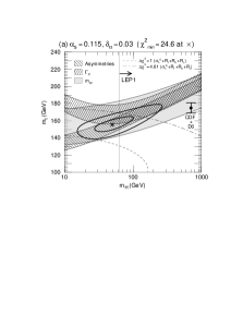
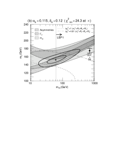
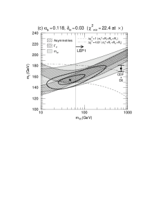
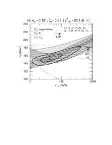
Figure 9: The SM fit to all electroweak data in the ($m_{H},\,m_{t}$) plane for various choices of $(\alpha_{s},\delta_{\alpha})$ : (a) (0.115,0.03) , (b) (0.115,0.012) , (c) (0.118,0.03) , (d) (0.118,0.012) , (e) (0.121,0.03) , (f) (0.121,0.012) , where $\delta_{\alpha}=1/\bar{\alpha}(m_{Z}^{2})-128.72$[2]. The thick inner and outer contours correspond to $\Delta\chi^{2}=1$ ($\sim$ 39% CL), and $\Delta\chi^{2}=4.61$ ($\sim$ 90% CL), respectively. The minimum of $\chi^{2}$ is marked by the sign “$\times$”. Also shown are the 1-$\sigma$ bands from the $Z$-pole asymmetries, $\Gamma_{Z}$ and $m_{W}$. The dashed lines show the constraint from the sum of $\sigma_{h}^{0}$, $R_{\ell}$, $R_{b}$ and $R_{c}$.

Throughout (5.1)–(5.1), the fitted $\alpha_{s}$ value agree well with the global average, $\alpha_{s}=0.118\pm 0.003$[28]. A slightly smaller value of $m_{H}\,(\sim 50{\,\rm GeV})$ is favored with the error of order 1 for $\log m_{H}$, and slightly smaller value of $m_{t}$ is favored as compared to the Tevatron measurement. The best-fit value of $m_{H}$ is sensitive to $\delta_{\alpha}$, whereas that of $m_{t}$ is sensitive to the $R_{b}$ data. The 4-parameter fit results given in Eqs. (5.1)–(5.1) are intended to illustrate qualitatively our understanding of the SM fit to the electroweak. The errors are not fully elliptic. More accurate constraints on these parameters can be obtained from the parametrization of the $\chi^{2}$-function given below in Eq. (10).

In conclusion, the fits are stable and agree with the a priori knowledge on $\alpha_{s}$ and $\delta_{\alpha}$. It is justified to proceed with an in-depth study based on the two parameters $m_{t}$ and $m_{H}$, where now $\alpha_{s}$ and $\delta_{\alpha}$ play the role of external parameters.

5.2 Constraints on $m_{t}$ and $m_{H}$ as functions of $\alpha_{s}$ and $\bar{\alpha}(m_{Z}^{2})$

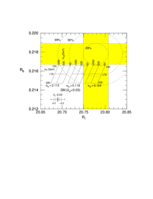
Figure 10: The $R_{b}$ vs $R_{\ell}$ plane. The SM predictions are shown in the range $120{\,\rm GeV}\!<\!m_{t}\!<\!240{\,\rm GeV}$, and $60{\,\rm GeV}\!<\!m_{H}\!<\!1{\,\rm TeV}$, for three cases of $\alpha_{s}$ ($\alpha_{s}$=$0.11$, $0.12$ and $0.13$). These predictions are for $\delta_{\alpha}=0.03$, and their dependences on $\delta_{\alpha}$ are also indicated. Also shown are the 39%, 90% and 99%CL contours obtained by combining only the $R_{\ell}$ and $R_{b}$ data.

In the minimal SM all relevant form factor values, i.e. $\bar{g}_{Z}^{2}(m_{Z}^{2})$, $\bar{s}^{2}(m_{Z}^{2})$, $\bar{g}_{Z}^{2}(0)$, $\bar{s}^{2}(0)$, $\bar{g}_{W}^{2}(0)$ and $\mbox{$\bar{\delta}_{b}$}(m_{Z}^{2})$, are predicted uniquely in terms of on the two mass parameters $m_{t}$ and $m_{H}$. A convenient parametrization of the SM contributions to these form factors is given in Eqs. (2)–(2), as functions of $\mbox{$x_{t}$}=(m_{t}({\,\rm GeV})-175)/10$, $\mbox{$x_{H}$}=\log(m_{H}({\,\rm GeV})/100)$ together with $\alpha_{s}$ and $\delta_{\alpha}$. Figure 9 shows the result of the fit to all electroweak data in the ($m_{H},\,m_{t}$)-plane for choices of $\alpha_{s}$ and $\delta_{\alpha}$ representative of their present knowledge. The figure exhibits to what extent the best-fit values as well as the size and orientation of the corresponding error ellipses ($\Delta\chi^{2}\equiv\chi^{2}-\chi^{2}_{\rm min}=$ 1 and 4.61) depend on the knowledge of the external parameters $\alpha_{s}$ and $\delta_{\alpha}$.

In order to understand how the fit comes about the 1-$\sigma$ constraints from the individual observables are shown separately. The narrow “asymmetry” band is sensitive to $\delta_{\alpha}$, whereas the “$\Gamma_{Z}$” band is sensitive to $\alpha_{s}$. The asymmetries constrain $m_{t}$ and $m_{H}$ through $\bar{s}^{2}(m_{Z}^{2})$, while $\Gamma_{Z}$ does so through all the three form factors $\bar{g}_{Z}^{2}(m_{Z}^{2})$, $\bar{s}^{2}(m_{Z}^{2})$ and $\mbox{$\bar{\delta}_{b}$}(m_{Z}^{2})$. It is most remarkable[3] that in the SM $\Gamma_{Z}$ depends upon almost the same combination of $m_{t}$ and $m_{H}$ as the one measured through $\bar{s}^{2}(m_{Z}^{2})$ provided $m_{H}$ is larger than about 60 GeV, which is indeed the range not excluded by the LEP1 experiments. The reason can be traced back to the approximate cancellation of the quadratic $m_{t}$-dependence of $\bar{g}_{Z}^{2}(m_{Z}^{2})$ and $\bar{\delta}_{b}$. Thus, the asymmetries and $\Gamma_{Z}$ alone, despite their quite small experimental errors, are constraining only a narrow band in the ($m_{t}$,$m_{H}$)-plane. The present constraint due to the $m_{W}$ measurement overlaps this band.

Additional information is required to disentangle the above $m_{t}$-$m_{H}$ correlation. This is provided by $R_{\ell}$, $\sigma_{h}$, $R_{b}$ and is shown in Fig. 9 by dashed lines corresponding to a $\Delta\chi^{2}$ of 1 ($\sim$39% CL) and 4.61 ($\sim$90% CL). The constraints due to $R_{\ell}$ and $R_{b}$ can also be seen in Fig. 10. $R_{\ell}$ is sensitive to the assumed value of $\alpha_{s}$, and, for $\alpha_{s}=0.118$, the data favors small $m_{H}$. $R_{b}$ is neither sensitive to $\alpha_{s}$ nor $m_{H}$ and the present average disfavors large $m_{t}$.

Without the data on $R_{\ell}$, $\sigma_{h}$ and $R_{b}$ the region of large $m_{H}$-values in the ($m_{t},m_{H}$)-band of Fig. 9 $(m_{H}\sim 1{\,\rm TeV})$ would not be excluded at all, as far as the electroweak data are concerned. It is worth noting that in comparing Fig. 9 (a) with (e) (or (b) with (f)) the $\Gamma_{Z}$-band is shifted downwards by more than 10 GeV in the top quark mass when one increases $\alpha_{s}$ from 0.115 to 0.121, but despite of this shift the best-fit point moves only marginally downwards by about 1.7 GeV (see also the parametrization (5.2) below). This is mainly because the constraint from $\sigma_{h}^{0}$, $R_{\ell}$ and $R_{b}$ allows larger $m_{t}$ for larger $\alpha_{s}$, as can be seen from dashed contours in Fig. 9, or from Fig. 10. The fit improves slightly at larger $\alpha_{s}$, because the $\Gamma_{Z}$ constraint then favors lower $m_{t}$ which in turn is favored by the $R_{b}$ data. On the other hand the change in $\delta_{\alpha}$ from the mean value of the estimate of Ref. [18], 0.03, to that of Ref. [16], 0.12, lowers the best-fit $m_{t}$ value by about 5 GeV and enhances that of $m_{H}$ slightly (by about 15 GeV), whereas the overall fit quality remains unchanged. The $\chi^{2}$ function of the fit to all electroweak data can be parametrized in terms of the four parameters $m_{t}$, $m_{H}$, $\alpha_{s}$ and $\delta_{\alpha}$ :

$$\chi^{2}_{\rm SM}(m_{t},m_{H},\alpha_{s},\delta_{\alpha}) = \biggl{(}\frac{m_{t}-\langle m_{t}\rangle}{\Delta m_{t}}\biggr{)}^{2}+\chi^{2}_{H}(m_{H},\alpha_{s},\delta_{\alpha})\,,$$ (5.51a)

with

$$\langle m_{t}\rangle = 162.4+13.0\,\log\frac{m_{H}}{100}+0.8\,\log^{2}\frac{m_{H}}{100}-0.85\,\biggl{(}\frac{\alpha_{s}-0.118}{0.003}\biggr{)}-4.9\,\biggl{(}\frac{\delta_{\alpha}-0.03}{0.09}\biggr{)},$$

$$\Delta m_{t} = 5.5-0.06\,\log\frac{m_{H}}{100}-\Bigl{(}0.090-0.018\,\log\frac{m_{H}}{100}\Bigr{)}\,\frac{m_{t}-175}{6}\,,$$ (5.51c)

and

$$\chi^{2}_{H}(m_{H},\alpha_{s},\delta_{\alpha}) = 22.1+\biggl{(}\frac{\delta_{\alpha}-0.19}{0.18}\biggr{)}^{2}+\biggl{(}\frac{\alpha_{s}-0.1201+0.0011\,\delta_{\alpha}}{0.0031}\biggr{)}^{2}\quad$$

$$-\biggl{(}\frac{\alpha_{s}-0.1343+0.063\,\delta_{\alpha}}{0.0071}\biggr{)}\log\frac{m_{H}}{100}-\biggl{(}\frac{\alpha_{s}-0.1305}{0.0129}\biggr{)}\log^{2}\frac{m_{H}}{100}\,.$$

Here $m_{t}$ and $m_{H}$ are measured in GeV, and ${\rm d.o.f}=25$. This parametrization reproduces the exact $\chi^{2}$ function within a few percent accuracy in the range $100{\,\rm GeV}<m_{t}<250{\,\rm GeV}$, $60{\,\rm GeV}<m_{H}<1000{\,\rm GeV}$ and $0.10<\alpha_{s}(m_{Z})<0.13$. The best-fit value of $m_{t}$ for a given set of $m_{H}$, $\alpha_{s}$ and $\delta_{\alpha}$ is readily obtained from Eq. (LABEL:fitofmtbest) with its approximate error of (5.51c). See dotted curves in Fig. 11.

Figure 11: Total $\chi^{2}$ of the SM fit to all the electroweak data as functions of $m_{t}$ for $m_{H}=60$, 300, 1000${\,\rm GeV}$ and $\alpha_{s}(m_{Z})=0.112,\,0.118,\,0.124$. The uncertainty $\delta_{\alpha}$ in the hadronic vacuum polarization contribution to the effective charge $1/\bar{\alpha}(m_{Z}^{2})$ is shown for three cases, $\delta_{\alpha}=-0.06$ (a), $0.03$ (b), $+0.12$ (c). The dotted lines are obtained by using the approximate formula (10). The number of degrees of freedom is 25.

Figure 12: Total $\chi^{2}$ of the SM fit to all the electroweak data as functions of $m_{H}$ when $m_{t}$ is allowed to vary, with $\alpha_{s}(m_{Z})=0.118\pm 0.003$[28] for $\delta_{\alpha}=0.03\pm 0.09$[18] (a) and $\delta_{\alpha}=0.12\pm 0.06$[16] (b). Results for various sets of the electroweak data with or without the Tevatron $m_{t}$ data, $m_{t}=175\pm 6{\,\rm GeV}$[8] are given. The degrees of freedom is 25 for ‘All EW $+m_{t}$’ case.

For $m_{H}=60,300,1000{\,\rm GeV}$, $\alpha_{s}=0.118\pm 0.03$ and $\delta_{\alpha}=0.03\pm 0.09$, one obtains

$$m_{t}=178\pm 6{}^{+19(m_{H}=1000)}_{-21(m_{H}=60)}\mp 1(\alpha_{s})\mp 5(\delta_{\alpha})\,,$$ (5.52)

where the mean value is for $m_{H}=300$ GeV. The fit (5.52) agrees with the best value from CDF and D0

$$m_{t}=175\pm 6~{}{\,\rm GeV}.$$ (5.53)

This agreement strongly suggests that the electroweak theory respects the gauge invariance, since otherwise the quantum corrections could not be calculated. An elaboration on this point follows in the next subsection. Furthermore, the successful prediction of $m_{t}$ based on the simple SM radiative corrections strongly supports the presence of the custodial SU(2) symmetry as part of physics responsible for spontaneous symmetry breaking. Without custodial SU(2) there would have been no prediction for $m_{t}$. Furthermore, the mechanism that leads to the large mass splitting of the third generation quarks should give rise to a $T$ value which is similar to its standard model value. Therefore, the success of the SM prediction not only suggests the presence of the custodial SU(2) symmetry, but also constrains the mechanism of the fermion mass generation.

Due to the quadratic form of Eq. (10) one can readily integrate out the unwanted terms, for instance those containing $\alpha_{s}$ and/or $\delta_{\alpha}$, and render the result independent of them. Also, additional constraints on the external parameters $\alpha_{s}$ and $\delta_{\alpha}$, such as those from future improved measurements or the constraint from the grand unification of these couplings may be added without difficulty.

As discussed above, the value for $m_{H}$ resulting from the Standard Model fit is correlated with the value of mt. The present value for $R_{b}$ which disfavors large masses of the top quark induces therefore a small value of the Higgs mass. It should also be noted that the choice of the value of $\alpha_{s}$ as an external parameter implies via Eq. (4.1) a constraint on the vertex form factor $\bar{\delta}_{b}$ and influences in turn the fit value for $m_{H}$. Shown in Fig. 12 are the $m_{H}$-dependence of $\chi^{2}$ under various assumptions. We present in Table 6 the corresponding 95%CL upper and lower bounds on $m_{H}$(GeV) from the electroweak data. A low mass Higgs boson is clearly favored. However, this trend disappears for $\alpha_{s}=0.118\pm 0.003$[28], once we ignore the $R_{b}$ data. If we adopt the estimate $\delta_{\alpha}=0.03\pm 0.09$[18] for $\bar{\alpha}(m_{Z}^{2})$, the 95%CL upper bound on $m_{H}$ is $270{\,\rm GeV}$ from all the $Z$ boson data, while it weakens to $1200{\,\rm GeV}$, if the $R_{b}$ data are ignored. The corresponding upper bounds with the estimate $\delta_{\alpha}=0.12\pm 0.06$[16] are $370{\,\rm GeV}$ and $1900{\,\rm GeV}$, respectively. An addition of the low energy neutral current data slightly lowers the upper $m_{H}$ bound, mainly because the combined fit, (4.3), gives slightly smaller $\bar{g}_{Z}^{2}(m_{Z}^{2})$, i.e. smaller $T$, than the $Z$ parameters would give alone. Just like smaller $R_{b}$ favors smaller $m_{t}$, smaller $T$ favors smaller $m_{t}$ and through the strong $m_{t}$ and $m_{H}$ correlation from the $\Gamma_{Z}$ and the asymmetry data smaller $m_{H}$ is favored. It is hence the direct measurement from the Tevatron, $m_{t}=175\pm 6{\,\rm GeV}$, that essentially constrains the allowed $m_{H}$, $m_{H}<480{\,\rm GeV}$ for $\delta_{\alpha}=0.03\pm 0.12$ or $m_{H}<590{\,\rm GeV}$ for $\delta_{\alpha}=0.09\pm 0.06$ at 95%CL, given the $\Gamma_{Z}$ and the asymmetry constraint.

Table 6: 95%CL upper and lower bounds of $m_{H}$(GeV) for $\alpha_{s}=0.118\pm 0.003$[28], $\delta_{\alpha}=0.03\pm 0.09$[18] or $\delta_{\alpha}=0.12\pm 0.06$[16]. Results for various sets of the electroweak data with or without the Tevatron $m_{t}$ data, $m_{t}=175\pm 6{\,\rm GeV}$[8] are given.

	$\alpha_{s}=0.118\pm 0.003$
	$\delta_{\alpha}=0.03\pm 0.12$				$\delta_{\alpha}=0.12\pm 0.06$
	best-fit	lower bound	upper bound	$\chi^{2}_{\rm min}$	best-fit	lower bound	upper bound	$\chi^{2}_{\rm min}$
EW$\,+\,m_{t}$	170	46	480	24.9	240	87	590	24.6
EW$\,+\,m_{t}\,-\,R_{b}$	200	54	550	21.4	280	100	670	21.1
EW	51	17	270	17.1	67	21	370	17.1
EW$\,-\,R_{b}$	60	17	730	20.4	90	22	1200	20.4
$Z$	51	17	270	17.1	67	21	370	17.1
$Z\,-\,R_{b}$	72	18	1200	15.2	120	24	1900	15.2
$Z\,-\,A_{\rm FB}^{b,0}$	30	11	140	11.9	38	13	200	11.6
$Z\,-\,A_{\rm LR}^{0}$	82	23	450	10.9	110	29	590	11.1

Table 7: 95%CL upper and lower bounds of $m_{H}$(GeV) when $m_{t}$ is fixed externally. Two estimates of $\bar{\alpha}(m_{Z}^{2})$ are examined, $\delta_{\alpha}=0.03\pm 0.09$[18] and $\delta_{\alpha}=0.12\pm 0.06$[16], for $\alpha_{s}=0.118\pm 0.003$[28].

	$\alpha_{s}=0.118\pm 0.003$
	$\delta_{\alpha}=0.03\pm 0.09$				$\delta_{\alpha}=0.12\pm 0.06$
$m_{t}$	best-fit	lower bound	upper bound	$\chi^{2}_{\rm min}$	best-fit	lower bound	upper bound	$\chi^{2}_{\rm min}$
160	72	22	190	22.7	110	45	240	22.6
165	110	33	260	23.4	150	67	320	23.3
170	150	54	360	24.3	220	99	430	24.0
175	220	87	490	25.3	300	140	580	24.9
180	310	130	660	26.4	410	210	780	26.0
185	430	200	900	27.6	550	290	1000	27.1
190	590	280	1200	28.9	740	390	1400	28.5

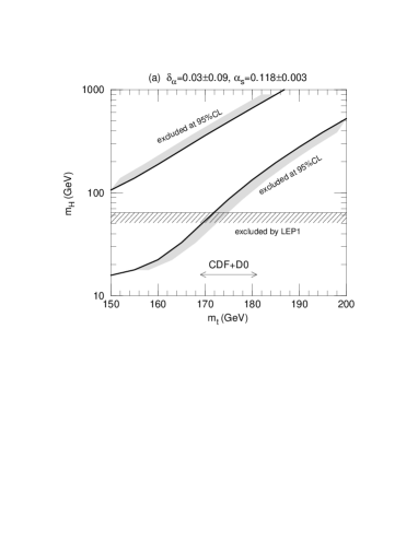
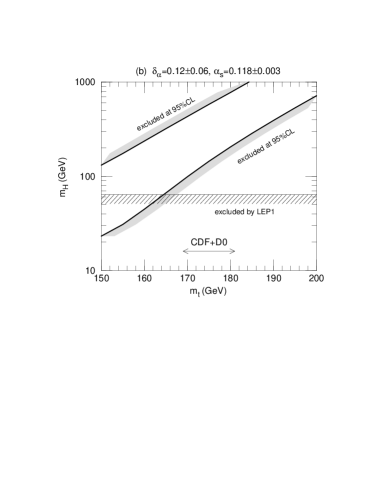
Figure 13: Constraints on the Higgs mass in the SM from all the electroweak data. Upper and lower bounds of the Higgs mass at 95% CL are shown as functions of the top mass $m_{t}$, where $m_{t}$ is treated as an external parameter with negligible uncertainty. The results are shown for $\alpha_{s}=0.118\pm 0.003$[28] and for $\delta_{\alpha}=0.03\pm 0.09$[18] (a) and $\delta_{\alpha}=0.12\pm 0.06$[16] (b). Also shown are the direct lower bound on $m_{H}$ from LEP1 and the Tevatron data $m_{t}=175\pm 6{\,\rm GeV}$[8].

The constraints on $m_{H}$ become much stronger once the top quark mass is known precisely, either due to more precise measurements or due to deeper theoretical insight. Lower and upper bounds on $m_{H}$ are shown in Fig. 13 and in Table 7 as functions of $m_{t}$ for the two estimates of $\bar{\alpha}(m_{Z}^{2})$. With the estimate of E-J[18], $\delta_{\alpha}=0.03\pm 0.12$, a lower $m_{H}$ is favored ($m_{H}<360{\,\rm GeV}$ at 95%CL), if $m_{t}<170{\,\rm GeV}$, while an intermediate $m_{H}$ is favored ($m_{H}>140{\,\rm GeV}$ at 95%CL) for $m_{t}>180{\,\rm GeV}$. With the estimate of M-Z[16], $\delta_{\alpha}=0.12\pm 0.06$, similar constraints are found at about $5{\,\rm GeV}$ smaller $m_{t}$. It is hence rather crucial for models where the Higgs boson is light (e.g. $m_{H}<130{\,\rm GeV}$ in the MSSM[42]) to have $m_{t}$ smaller than the actual present mean value, $m_{t}\sim 175{\,\rm GeV}$.

Finally, we repeat the 4-parameter fits, (5.1)–(5.1) on the electroweak data when the direct $m_{t}$ measurement, $m_{t}=175\pm 6{\,\rm GeV}$ (Tevatron), is taken into account. Without external constraints on $\alpha_{s}$ and $\delta_{\alpha}$, we find

$$\!\!\left.\begin{array}[]{c@{\,}r@{\,}l}m_{t}({\,\rm GeV})&=&173\pm 6\\[2.84526pt] \mbox{$x_{H}$}&=&1.7\pm 1.1\\[2.84526pt] \alpha_{s}&=&0.1218\pm 0.0037\\[2.84526pt] \delta_{\alpha}&=&0.30\pm 0.26\end{array}\right\}\;\rho_{\rm corr}=\left(\begin{array}[]{rrrr}1.0&0.4&0.2&-0.1\\ &1.0&0.5&-0.9\\ &&1.0&-0.4\\ &&&1.0\end{array}\right),\,\,\,\qquad$$ (5.54i)

$$\chi^{2}_{\rm min}/({\rm d.o.f.})=23.8/(22)\,.$$ (5.54j)

The top quark mass appears now basically determined by the direct measurement, while the mean $\delta_{\alpha}$ grows considerably and, consequently, a larger $m_{H}$, $m_{H}=530^{+1600}_{-170}{\,\rm GeV}$ is favored. The shifted best value of $m_{t}$ slightly affects the sensitivity to $\alpha_{s}$ (see Eq. (5.1)). The value of $\alpha(m_{Z}^{2})$ obtained from the electroweak measurements agrees roughly with that of Ref.[37], which may be expressed as $\delta_{\alpha}=0.21^{+0.25}_{-0.32}$.

Adding the external constraint $\alpha_{s}=0.118\pm 0.003$ [28] does not significantly alter the situation, because the fit (13) results in the $\alpha_{s}$ value consistent with the world average.

Because the best-fit value of $\delta_{\alpha}$ in (13) is slightly larger than the estimate $\delta_{\alpha}=0.03\pm 0.09$ by E-J[18], the strong negative correlation between $\Delta\delta_{\alpha}$ and $\Delta\mbox{$x_{H}$}$ in (13) entails a sizeably lower $m_{H}$:

$$\!\!\left.\begin{array}[]{c@{\,}r@{\,}l}m_{t}({\,\rm GeV})&=&171\pm 6\\[2.84526pt] \mbox{$x_{H}$}&=&0.5\pm 0.6\\[2.84526pt] \alpha_{s}&=&0.1191\pm 0.0022\\[2.84526pt] \delta_{\alpha}&=&0.05\pm 0.08\end{array}\right\}\;\rho_{\rm corr}=\left(\begin{array}[]{rrrr}1.0&0.6&0.1&-0.0\\ &1.0&0.2&-0.6\\ &&1.0&-0.1\\ &&&1.0\end{array}\right),\,\,\,\qquad$$ (5.55i)

$$\chi^{2}_{\rm min}/({\rm d.o.f.})=24.9/(24)\,.$$ (5.55j)

Since the four parameter fits are not fully elliptic, we show in Fig. 14 both the 1-$\sigma$ and 90%CL allowed regions in the $(m_{H},\,m_{t})$ plane by solid contours. The 1-$\sigma$ preferred range $m_{H}=170^{+150}_{-90}{\,\rm GeV}$ agrees roughly with the estimates of Refs.[1, 39, 40]. Similar results with slightly larger $m_{H}$ are found, if we adopt the M-Z estimation[16] $\delta_{\alpha}=0.12\pm 0.06$:

$$\!\!\left.\begin{array}[]{c@{\,}r@{\,}l}m_{t}({\,\rm GeV})&=&172\pm 6\\[2.84526pt] \mbox{$x_{H}$}&=&0.9\pm 0.6\\[2.84526pt] \alpha_{s}&=&0.1193\pm 0.0022\\[2.84526pt] \delta_{\alpha}&=&0.12\pm 0.06\end{array}\right\}\;\rho_{\rm corr}=\left(\begin{array}[]{rrrr}1.0&0.7&0.1&-0.0\\ &1.0&0.2&-0.4\\ &&1.0&-0.1\\ &&&1.0\end{array}\right),\,\,\,\qquad$$ (5.56i)

$$\chi^{2}_{\rm min}/({\rm d.o.f.})=24.6/(24)\,.$$ (5.56j)

The corresponding allowed ranges in the $(m_{H},\,m_{t})$ plane are given by dashed contours in Fig. 14. The preferred $m_{H}$ range is now $m_{H}=240^{+180}_{-110}{\,\rm GeV}$. We note here that once the external $m_{t}$ data is included in the fit, the relative importance of the $R_{b}$ on the SM fit decreases. The above fit (13) and (5.2) are barely affected by excluding the $R_{b}$ data.

The above exercises demonstrate well the overall consistency of the electroweak radiative corrections in the SM and emphasize at the same time the importance of an improved $\bar{\alpha}(m_{Z}^{2})$ estimate for constraining $m_{H}$ in fits based on electroweak precision experiments.

Figure 14: The SM fit to all electroweak data in the ($m_{H},\,m_{t}$) plane with external constraints on $m_{t}$ from Tevatron, $m_{t}=175\pm 6{\,\rm GeV}$[8], $\alpha_{s}=0.118\pm 0.003$[28], and two estimates[18, 16] for $\delta_{\alpha}=1/\bar{\alpha}(m_{Z}^{2})-128.72$. The inner and outer contours correspond to $\Delta\chi^{2}=1$ ($\sim$ 39% CL), and $\Delta\chi^{2}=4.61$ ($\sim$ 90% CL), respectively. The minimum of $\chi^{2}$ is marked by the sign “$\times$” for the $\bar{\alpha}(m_{Z}^{2})$ estimate of [18] and by the sign “$+$” for the estimate [16]. Also shown is the direct lower bound on $m_{H}$ from LEP1.

5.3 Is there already indirect evidence for the standard $W$ self-coupling?

The success of the SM in describing all precision electroweak experiments at the quantum level may be taken as indirect evidence of the non-Abelian nature of the electroweak theory, or respectively of the standard universal gauge-boson self-couplings, because it is the non-Abelian gauge symmetry of the SM which ensures its renormalizability.

Any alternative[43] to gauge models should necessarily have the new physics (cut-off) scale of order $m_{W}$, whereas the universality of the weak interactions may be associated with the underlying symmetry of the fundamental theory and the vector boson dominance which require relatively high ($\gg m_{W}$) scales for new physics. The fact that the SM works well at the quantum level indicates that the weak boson interactions do not deviate significantly from their gauge theory form at least up to the scale of $2m_{t}$. Therefore, it is instructive to study in more detail which part of the standard radiative corrections is supported by experiment and whether indeed there is evidence for the gauge boson self-couplings.

It is not straightforward to answer this question, since we have to identify which finite portion of the quantum corrections is sensitive to the weak-boson self-interactions. Usually one splits the complete SM radiative corrections into just two separately gauge invariant pieces, namely the fermionic loop contributions to the gauge-boson self-energies and the rest. It can then be stated unambiguously that neither of the corrections alone is sufficient to describe the data, and that only the inclusion of both contributions ensures the success of the SM radiative corrections[44]. As a matter of fact, the bosonic part of the correction contains the weak boson self-interactions as an essential part and in this sense it is indirect evidence for universal couplings.

In a more detailed attempt[45] at understanding the importance of bosonic contributions due to the $WWZ$ and $WW\gamma$ couplings, it should be elucidated to what extent these finite bosonic correction terms depend on the splitting of the gauge bosons into themselves. For instance, the box diagrams do not contain gauge-boson self-couplings. It is useful to split the bosonic corrections into three separately gauge-invariant pieces, namely ‘box-like’, ‘vertex-like’ and ‘propagator-like’ pieces by appealing to the S-matrix pinch technique[10]. It is then only the ‘vertex-like’ and ‘propagator-like’ pieces which contain the gauge boson self-couplings. Schematically we separate the SM radiative corrections into the following five pieces:

$$\begin{array}[]{lll@{\quad\hspace{1mm}\quad}l}{\cal M}\quad=&\quad\mbox{QED/QCD}&\hfil\quad\hskip 2.84526pt&(A)\\[0.85358pt] &\mbox{+ fermion-loop}&\begin{picture}(40.0,20.0)(2.0,8.0) \put(0.0,0.0){} \put(0.0,0.0){} \put(0.0,0.0){} \put(0.0,0.0){} \end{picture}\hfil\quad\hskip 2.84526pt&(B)\\[0.85358pt] &\mbox{+ box}&\begin{picture}(40.0,20.0)(-12.0,8.0) \put(0.0,0.0){} \put(0.0,0.0){} \put(0.0,0.0){} \put(0.0,0.0){} \end{picture}\hfil\quad\hskip 2.84526pt&(C)\\[0.85358pt] &\mbox{+ vertex}&\begin{picture}(40.0,20.0)(-12.0,8.0) \put(0.0,0.0){} \put(0.0,0.0){} \put(0.0,0.0){} \end{picture}+\begin{picture}(40.0,20.0)(-12.0,8.0) \put(0.0,0.0){} \put(0.0,0.0){} \put(0.0,0.0){} \put(0.0,0.0){} \end{picture}\hfil\quad\hskip 2.84526pt&(D)\\[0.85358pt] &\mbox{+ bosonic-loop}&\begin{picture}(45.0,20.0)(2.0,8.0) \put(0.0,0.0){} \put(0.0,0.0){} \put(0.0,0.0){} \put(0.0,0.0){} \put(0.0,0.0){} \put(0.0,0.0){} \end{picture}+\begin{picture}(40.0,20.0)(5.0,8.0) \put(0.0,0.0){} \put(0.0,0.0){} \end{picture}+\begin{picture}(45.0,15.0)(2.0,8.0) \put(0.0,0.0){} \put(0.0,0.0){} \put(0.0,0.0){} \put(0.0,0.0){} \put(0.0,0.0){} \put(0.0,0.0){} \end{picture}\hfil\quad\hskip 2.84526pt&(E)\end{array}$$ (5.62)

Details of this separation for each radiative correction term may be obtained straightforwardly from the analytic expressions presented in Ref.[2]. By confronting these ‘predictions’ with the electroweak data the results of Table 8 are obtained.

The ‘no-EW’ entry confronts the tree-level predictions of the SM where only QCD and external QED corrections $(A)$ are applied. In this column $\bar{\alpha}(m_{Z}^{2})$ is calculated by including only contributions from light quarks and leptons with $\delta_{h}=0.03$[2, 18] for the hadronic uncertainty. It is quite striking to re-confirm the observation[41] that these ‘no-EW’ predictions agree well with experiments at LEP1/SLC. In fact, it reduces the $\chi^{2}$ over the SM, partly because of the $R_{b}$ data, which prefer no electroweak corrections $\mbox{$\bar{\delta}_{b}$}(m_{Z}^{2})=0$ compared to the SM prediction $\mbox{$\bar{\delta}_{b}$}(m_{Z}^{2})=-0.00995$ for $m_{t}=175{\,\rm GeV}$. It is only the $m_{W}$ value[46] and the $Z$ boson width which give significantly higher $\chi^{2}$ compared to the SM.

This can be understood as follows[45]. The three most accurately constrained electroweak parameters are $\bar{s}^{2}(m_{Z}^{2})$ from the asymmetries, $\bar{g}_{Z}^{2}(m_{Z}^{2})$ from $\Gamma_{Z}$ at LEP1/SLC experiments, and $m_{W}$ from Tevatron experiments. In terms of the ‘observable’ combinations $(S^{\prime},T^{\prime},U^{\prime})$ of Eq. (3), they can be expressed as

$$\bar{g}_{Z}^{2}(0) \approx 0.5456+0.0040T^{\prime}\,$$ (5.63a)

$$\bar{s}^{2}(m_{Z}^{2}) \approx 0.2324+0.0036S^{\prime}-0.0024T^{\prime}\,$$ (5.63b)

$$m_{W}({\,\rm GeV}) \approx 79.84-0.28S^{\prime}+0.42T^{\prime}+0.33U^{\prime}-0.29(T^{\prime}-T)\,.$$ (5.63c)

In the absence of electroweak corrections, the predictions are obtained by setting $S=T=U=\bar{\delta}_{G}=0$ and also by setting $\bar{g}_{Z}^{2}(m_{Z}^{2})-\bar{g}_{Z}^{2}(0)=0$. The purely light flavor value of $1/\bar{\alpha}(m_{Z}^{2})=1/\alpha(m_{Z}^{2})_{\rm l.f.}=128.89$ (see Table 4) corresponds to $\mbox{$\delta_{\alpha}$}=0.17$. These input values give rise to $(S^{\prime},T^{\prime},U^{\prime})=(-0.12,0.75,-0.04)$ which is not far from their SM values $(-0.23,0.88,0.36)$ for $m_{t}=175{\,\rm GeV}$, $m_{H}=100{\,\rm GeV}$ and $\bar{\delta}_{G}=0.0055$, or from the $(S,T,U)$ fit result of Eq. (8). The ‘no-EW’ case thus gives almost the same predictions for the three charge form factors, $\bar{g}_{Z}^{2}(0)$, $\bar{s}^{2}(m_{Z}^{2})$, and $\bar{g}_{W}^{2}(0)$ with those of the SM. All the asymmetry data at LEP1/SLC are hence reproduced well. The low energy neutral current experiments are also reproduced well, since the running of the $\bar{s}^{2}(q^{2})$ charge below the $m_{Z}$ scale is essentially governed by the ‘QED’ effects. The ‘no-EW’ model predicts significantly smaller $\Gamma_{Z}$ by about 3 to 4 $\sigma$ for $\alpha_{s}=0.118\pm 0.003$, because the running of the $\bar{g}_{Z}^{2}$ charge, $\bar{g}_{Z}^{2}(m_{Z}^{2})-\bar{g}_{Z}^{2}(0)\sim 0.05$ has been ignored. Furthermore, it fails to predict the measured $m_{W}$-value by about 3 $\sigma$, because its prediction is sensitive directly to the $\mu$ decay correction factor $\bar{\delta}_{G}$ in Eq. (3.8). This results in the last term in Eq. (5.63c), $-0.29(T^{\prime}-T)$, which lowers the $m_{W}$ prediction by more than 300 MeV.

The next ‘${\rm+fermion}$’ column gives the result of $(A)+(B)$ in Eq. (5.62). If we include only the fermionic corrections the $T$ parameter grows from zero to 1.14, while the factor $\bar{\delta}_{G}$ remains zero. The combination $T^{\prime}$ then becomes $T^{\prime}=1.14+0.75=1.89$ which gives a too large $\bar{g}_{Z}^{2}(0)$ and a too small $\bar{s}^{2}(m_{Z}^{2})$ as can be read off from Eq. (5.3). The fermionic loop gives a dominant contribution to the running of $\bar{g}_{Z}^{2}$ below $m_{Z}$, and the resulting $\bar{g}_{Z}^{2}(m_{Z}^{2})\approx\bar{g}_{Z}^{2}(0)+0.005$ makes the $Z$ boson width unacceptably large. From Table 8, we find that about half of $\chi^{2}\sim 500$ in the ‘$+$fermion’ entry comes from $\Gamma_{Z}$ and the rest from the LEP1/SLC asymmetries. In contrast, we find excellent agreement for $m_{W}$ in the same column. This is mainly because $m_{W}$ is more sensitive to $T$ rather than to $\bar{\delta}_{G}$ when $\alpha$, $G_{F}$ and $m_{Z}$ are fixed: $0.42T^{\prime}-0.29(T^{\prime}-T)=0.42T+0.13(T^{\prime}-T)$. Even though there are fortuitous cancellations among the remaining terms, we find no further improvement in the $m_{W}$ fit by adding extra radiative effects.

It turned out that the ‘box-like’ corrections to the $\mu$-decay matrix elements amount to almost 80% of the total $\bar{\delta}_{G}$ value:

$$[\bar{\delta}_{G}]_{\rm SM} = \bar{\delta}_{G}^{\rm box}+\bar{\delta}_{G}^{\rm vertex}\,,$$ (5.64a)

$$\bar{\delta}_{G}^{\rm box} = \frac{\hat{g}_{Z}^{2}}{16\pi^{2}}\Bigl{(}\frac{5}{2}-5\hat{s}^{2}+\hat{s}^{4}\Bigr{)}\frac{m_{W}^{2}}{m_{Z}^{2}-m_{W}^{2}}\log\frac{m_{Z}^{2}}{m_{W}^{2}}\,,$$ (5.64b)

$$\bar{\delta}_{G}^{\rm vertex} = \frac{\hat{g}^{2}\hat{c}^{2}}{16\pi^{2}}\Bigl{(}2-\frac{m_{Z}^{2}+m_{W}^{2}}{m_{Z}^{2}-m_{W}^{2}}\log\frac{m_{Z}^{2}}{m_{W}^{2}}\Bigr{)}+\frac{\hat{e}^{2}}{8\pi^{2}}\,.$$ (5.64c)

Hence by adding the ‘box-like’ corrections, $\bar{\delta}_{G}^{\rm box}=0.00429$, we have $(S^{\prime},T^{\prime},U^{\prime})=(-0.20,1.30,-0.02)$, and the fit improves significantly. The $T^{\prime}$ value is still slightly too large, and the ‘$+$box’ entry still gives too large $\Gamma_{Z}$ and too small $\bar{s}^{2}(m_{Z}^{2})$. This can be seen from the column of ‘${\rm+box}$’, where we give results of $(A)+(B)+(C)$ corrections in Eq. (5.62).

These electroweak effects do not affect much the fit of the low energy neutral current experiments because of their larger experimental errors. It is worth noting here that among the electroweak radiative corrections, the ’box-like’ ones, especially the $WW$-box contribution, are most significant in the atomic parity violation experiments. Indeed the fit for $Q_{W}(C_{s})$ improves significantly by adding the ’box-like’ corrections.

Up to this stage no contribution from quantum fluctuations with the weak-boson self-couplings are counted. Next the column ‘${\rm+vertex}$’ is considered, where the results of A+B+C+D corrections are listed and where we may hope to see their effects. It turns out that the effects of the remaining 20% correction to $\bar{\delta}_{G}$ and the effects in part from the vertex corrections in the $Z$-decay matrix elements considerably reduce the $\chi^{2}$ in the LEP1/SLC sector of the experiments from about 200 down to 30. The effect of the full $\bar{\delta}_{G}$ is to change the charge form factor inputs to $(S^{\prime},T^{\prime},U^{\prime})=(-0.20,1.14,-0.02)$, which reduces $\bar{g}_{Z}^{2}(m_{Z}^{2})$ by only 0.1%, increases $\bar{s}^{2}(m_{Z}^{2})$ by 0.2%. The predicted $\Gamma_{Z}$ is reduced by 1% and excellent agreement with the data is found (compare the relevant entries in the ‘$+$box’ and ‘$+$vertex’ entries). The major effect of the vertex corrections to $\Gamma_{Z}$ is actually coming from the corrections to the $Zff$ vertices in which the corrections from the diagrams with the $WWZ$ vertex, $\overline{\Gamma}^{f}_{2}$ in Table 3 of Ref. [2], are most significant. The prediction $\bar{s}^{2}(m_{Z}^{2})=0.22995$ is still by about 3-$\sigma$ away from the fit (2.2).

Inclusion of the ‘propagator-like’ corrections either improves or worsens the fit depending on the Higgs boson mass. The improvement is sizeable only when the Higgs boson mass is not too large, as can be seen from the last column in Table 8.

It is therefore tempting to conclude that the effect of the ‘vertex-like’ corrections, and hence that of the standard $WWV$ self-interactions is essential for the success of the SM at the quantum correction level. Once the gauge invariance of the weak boson interactions is assumed, quantum fluctuations at very short distances become universal and hence they can be renormalized by precisely measured quantities. Remaining finite parts of the quantum corrections hence measure the effects of the intermediate scale physics which can be sensitive to the symmetry breaking physics. With further improvement of the electroweak data, we will therefore learn more about physics of 100 GeV to 1 TeV that could affect these finite correction terms. The precision electroweak physics may still give us hints of new physics at the energy region which is not yet explored directly by high energy experiments.

Table 8: The electroweak data and the SM predictions. The three predictions for $\Gamma_{Z}$, $\sigma_{h}^{0}$ and $R_{\ell}$ are for $\alpha_{s}=0.115$, 0.118 and 0.121.

	data	no-EW	+fermion	+box	+vertex	+propagator
$m_{t}$ (GeV)		——	175	175	175	175	175	175
$m_{H}$ (GeV)		——	100	——	100	60	300	1000
$S$		——	-0.067	-0.067	-0.067	-0.283	-0.146	-0.075
$T$		——	1.136	1.136	1.136	0.910	0.762	0.583
$U$		——	0.017	0.017	0.017	0.364	0.359	0.358
$\bar{\delta}_{G}$		——	——	0.00429	0.00549	0.00549	0.00549	0.00549
$1/\bar{\alpha}(m_{Z}^{2})$		128.89	128.90	128.90	128.90	128.75	128.75	128.75
$\bar{s}^{2}(m_{Z}^{2})$		0.23114	0.22815	0.22955	0.22995	0.23009	0.23094	0.23163
$\bar{g}_{Z}^{2}(m_{Z}^{2})$		0.54863	0.55812	0.55569	0.55502	0.55639	0.55592	0.55518
$\bar{\delta}_{b}(m_{Z}^{2})$		——	——	——	-0.00996	-0.00997	-0.00994	-0.01000
$\bar{s}^{2}(0)$		0.23866	0.23584	0.23716	0.23753	0.23850	0.23930	0.23995
$\bar{g}_{Z}^{2}(0)$		0.54863	0.55321	0.55083	0.55017	0.54926	0.54867	0.54795
$\bar{g}_{W}^{2}(0)$		0.42182	0.42713	0.42452	0.42379	0.42449	0.42339	0.42238
$\Gamma_{Z}$(GeV)	2.4946 $\pm$ 0.0027	2.4836	2.5346	2.5198	2.4905	2.4963	2.4920	2.4868
		2.4853	2.5364	2.5215	2.4922	2.4980	2.4937	2.4885
		2.4870	2.5381	2.5233	2.4939	2.4997	2.4953	2.4902
$\sigma_{h}^{0}$(nb)	41.508 $\pm$ 0.056	41.507	41.500	41.502	41.489	41.490	41.493	41.496
		41.491	41.484	41.486	41.473	41.474	41.477	41.481
		41.475	41.468	41.470	41.457	41.458	41.461	41.465
$R_{\ell}$	20.778 $\pm$ 0.029	20.768	20.817	20.795	20.733	20.731	20.716	20.703
		20.788	20.837	20.815	20.753	20.751	20.736	20.723
		20.808	20.857	20.835	20.773	20.771	20.756	20.743
$A_{\rm FB}^{0,\ell}$	0.0174 $\pm$ 0.0010	0.0169	0.0224	0.0198	0.0175	0.0172	0.0157	0.0145
$A_{\tau}$	0.1401 $\pm$ 0.0067	0.1500	0.1732	0.1624	0.1516	0.1505	0.1439	0.1384
$A_{e}$	0.1382 $\pm$ 0.0076	0.1500	0.1732	0.1624	0.1516	0.1505	0.1439	0.1384
$R_{b}$	0.2178 $\pm$ 0.0011	0.2182	0.2181	0.2182	0.2156	0.2156	0.2157	0.2157
$R_{c}$	0.1715 $\pm$ 0.0056	0.1717	0.1719	0.1718	0.1722	0.1722	0.1721	0.1721
$A_{\rm FB}^{0,b}$	0.0979 $\pm$ 0.0023	0.1054	0.1219	0.1142	0.1064	0.1056	0.1008	0.0969
$A_{\rm FB}^{0,c}$	0.0735 $\pm$ 0.0048	0.0753	0.0883	0.0822	0.0764	0.0758	0.0721	0.0691
$\sin^{2}\theta^{lept}_{eff}(\langle Q_{\rm FB}\rangle)$	0.2320 $\pm$ 0.0010	0.2311	0.2282	0.2296	0.2309	0.2311	0.2319	0.2326
$A_{\rm LR}$	0.1542 $\pm$ 0.0037	0.1500	0.1732	0.1624	0.1516	0.1505	0.1438	0.1384
$A_{b}({\rm LR})$	0.863 $\pm$ 0.049	0.936	0.938	0.937	0.935	0.935	0.934	0.934
$A_{c}({\rm LR})$	0.625 $\pm$ 0.084	0.669	0.679	0.674	0.670	0.669	0.666	0.664
$\chi^{2}$	$(\alpha_{s}=0.115)\quad$	37.1	455.3	181.6	32.3	27.3	24.9	49.5
(d.o.f.=14)	$(\alpha_{s}=0.118)\quad$	32.4	475.3	194.0	29.0	26.5	21.6	43.4
	$(\alpha_{s}=0.121)\quad$	29.8	497.2	208.4	27.7	27.6	20.2	39.2
$g_{L}^{2}$	0.2980 $\pm$ 0.0044	0.2955	0.3027	0.3049	0.3067	0.3049	0.3036	0.3024
$g_{R}^{2}$	0.0307 $\pm$ 0.0047	0.0309	0.0307	0.0307	0.0298	0.0300	0.0301	0.0302
$\delta_{L}^{2}$	-0.0589 $\pm$ 0.0237	-0.0601	-0.0606	-0.0652	-0.0645	-0.0645	-0.0645	-0.0644
$\delta_{R}^{2}$	0.0206 $\pm$ 0.0160	0.0186	0.0184	0.0184	0.0179	0.0180	0.0180	0.0181
$\chi^{2}$		0.4	1.8	3.9	5.5	3.5	2.4	1.5
$K$ (CCFR)	0.5626 $\pm$ 0.0060	0.5519	0.5641	0.5685	0.5702	0.5673	0.5653	0.5632
$\chi^{2}$		3.2	0.1	1.0	1.6	0.6	0.2	0.0
$s^{2}_{eff}$	0.233 $\pm$ 0.008	0.239	0.236	0.235	0.229	0.230	0.231	0.231
$\rho_{eff}$	1.007 $\pm$ 0.028	1.000	1.008	1.016	1.015	1.013	1.012	1.011
$\chi^{2}$		0.6	0.1	0.1	0.4	0.2	0.1	0.1
$Q_{W}$	-71.04 $\pm$ 1.81	-74.73	-74.74	-72.96	-72.92	-73.01	-73.10	-73.14
$\chi^{2}$		4.2	4.2	1.1	1.1	1.2	1.3	1.3
$2C_{1u}-C_{1d}$	0.938 $\pm$ 0.264	0.709	0.725	0.730	0.729	0.724	0.721	0.718
$2C_{2u}-C_{2d}$	-0.659 $\pm$ 1.228	0.081	0.099	0.103	0.112	0.106	0.101	0.097
$\chi^{2}$		1.9	1.2	1.1	1.1	1.2	1.4	1.5
$m_{W}$ (GeV)	80.356 $\pm$ 0.125	79.957	80.459	80.384	80.363	80.429	80.325	80.229
$\chi^{2}$		10.2	0.7	0.0	0.0	0.3	0.1	1.0
$\chi^{2}_{\rm tot}$	$(\alpha_{s}=0.115)\quad$	57.6	463.3	188.8	41.9	34.4	30.3	54.9
(d.o.f.=25)	$(\alpha_{s}=0.118)\quad$	52.9	483.3	201.3	38.6	33.6	27.0	48.8
	$(\alpha_{s}=0.121)\quad$	50.3	505.2	215.7	37.3	34.7	25.7	44.7

6 Impact of future improved measurements

Constraints on various electroweak quantities are expected to be improved in the near future. Their impact on the knowledge of the top and the Higgs masses is discussed in the following subsections. The last subsection deals with future constraints on the $S$, $T$, $U$ parameters.

According to the discussions in the previous section the constraints on the top and the Higgs masses are basically obtained from three quantities, $\Gamma_{Z}$, $\bar{s}^{2}(m_{Z}^{2})$ from various $Z$-pole asymmetries, and $m_{W}$. After the completion of the LEP1 experiments no further improvement on $\Gamma_{Z}$ is expected. Significant improvements in $\bar{s}^{2}(m_{Z}^{2})$ may be expected from SLC, Tevatron, LHC, and future Linear $e^{+}e^{-}$ Colliders (LC). Improved measurements on $m_{W}$ are also expected from LEP2, Tevatron, LHC, and LC. The top quark mass will be measured accurately at Tevatron, LHC, and LC. The Higgs boson mass can be measured at LEP2, LHC and LC, provided it exists and its mass lies in the accessible energy range of these machines. Finally, a more precise value of $\bar{\alpha}(m_{Z}^{2})$ will be obtained from experiments at Novosibirsk, DA$\Phi$NE, B factories at KEK, SLAC and DESY, and possibly at the Beijing $\tau$-charm factory (BTCF).

In order to assess the impact of such future improvements in the electroweak sector, we found the following approximate formulae for the SM predictions useful:

$$\Gamma_{Z}({\,\rm MeV}) \approx 2497.1+(2.51-0.01\,\mbox{$x_{H}$})\,x_{t}-2.29\,\mbox{$x_{H}$}-0.65\,x_{H}^{2}$$ (6.65a)

$$\hphantom{2497.1}+0.6\,x_{\alpha}+1.6\,x_{s}\,,$$

$$\bar{s}^{2}(m_{Z}^{2}) \approx 0.23034-(0.000335-0.000001\,\mbox{$x_{H}$})\,x_{t}+0.000518\,\mbox{$x_{H}$}+0.000017\,x_{H}^{2}\quad$$ (6.65b)

$$\hphantom{0.23034}-0.00023\,x_{\alpha}+0.00001\,x_{s}\,,$$

$$m_{W}({\,\rm GeV}) \approx 80.400+(0.0635-0.0001\,\mbox{$x_{H}$})\,x_{t}-0.0603\,\mbox{$x_{H}$}-0.0062\,x_{H}^{2}$$ (6.65c)

$$\hphantom{80.400}+0.012\,x_{\alpha}-0.002\,x_{s}\,.$$

Here $x_{t}=(m_{t}-175{\,\rm GeV})/10{\,\rm GeV}$, $\mbox{$x_{H}$}=\log(m_{H}/100{\,\rm GeV})$, $x_{\alpha}=(\mbox{$\delta_{\alpha}$}-0.03)/0.09$, and $x_{s}=(\alpha_{s}-0.118)/0.003$. The approximations are valid to 0.2 MeV (6.65a), 0.00002 (6.65b) and 0.003 GeV(6.65c), respectively, in the region $|\mbox{$x_{t}$}|<1$, $|\mbox{$x_{\alpha}$}|<1$, $|\mbox{$x_{s}$}|<1$ and 70 GeV$<m_{H}<$700 GeV. It is instructive to recall that $\Gamma_{Z}$ and $m_{W}$ measure approximately the same combination of $m_{t}$, $m_{H}$ and $\delta_{\alpha}$: $x_{t}-0.9\,\mbox{$x_{H}$}+0.2\,x_{\alpha}$. The asymmetry parameter $\bar{s}^{2}(m_{Z}^{2})$ constrains a different combination, which may be approximated as $x_{t}-1.5\,\mbox{$x_{H}$}+0.7\,x_{\alpha}$. Therefore, we need improvements in both $m_{W}$ and $\bar{s}^{2}(m_{Z}^{2})$ to reduce the electroweak constraints on $m_{t}$ and $m_{H}$. With the improved direct determination of $m_{t}$, each of the above experiments will lead to a significantly better constraint on $m_{H}$. The $m_{H}$ constraint can be strengthened by more precise estimates of $\bar{\alpha}(m_{Z}^{2})$.

6.1 Asymmetries

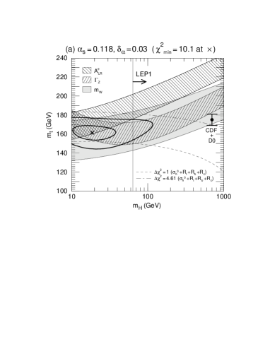
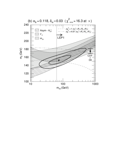
Figure 15: SM-fit using (a) only the left-right asymmetry by the SLD Collaboration and (b) using all other asymmetry data.

The different asymmetry measurements from LEP and SLC are in agreement with each other, although showing a large dispersion. The SLD collaboration has contributed the most precise individual determination, namely $\bar{s}^{2}(m_{Z}^{2})=0.2294\pm 0.0005$. The result is dominated by statistics and thus allows for substantial improvement. The average of all other measurements yields $\bar{s}^{2}(m_{Z}^{2})=0.2317\pm 0.0003$. It is instructive to repeat the above SM fit once with $A_{LR}^{0}$ alone and then with all other asymmetry data. Figure 15 shows the result in the $(m_{H},m_{t})$-plane. Due to the somewhat high value of $A_{LR}^{0}$, i.e. low value of $\bar{s}^{2}(m_{Z}^{2})$, the best-fit value for the Higgs mass turns out to be rather low and most of the allowed region is already excluded by the result of the Higgs searches at LEP1. The complementary fit leads to a best-fit Higgs mass of about 75 GeV, but with a low value for the top quark mass of 152 GeV. The 90% CL allowed region overlaps significantly with the direct information on $m_{H}$ and $m_{t}$. The change in size and orientation of the error ellipses can be understood by considering the SM grid in Fig. 3.

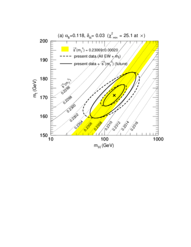
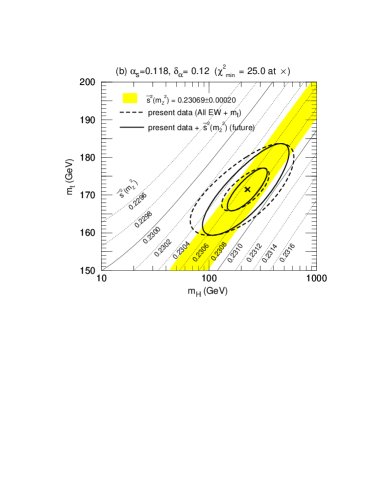
Figure 16: Impact of future improvement in $\bar{s}^{2}(m_{Z}^{2})$ in the ($m_{H},\,m_{t}$) plane, for $\alpha_{s}=0.118$ and $\delta_{\alpha}=0.03$(a), $\delta_{\alpha}=0.12$(b). An assumed future data $\bar{s}^{2}(m_{Z}^{2})=0.23069\pm 0.00020$ is used to constrain $m_{t}$ and $m_{H}$ in addition to the present all electroweak data and the Tevatron $m_{t}$ data, $m_{t}=175\pm 6{\,\rm GeV}$. The inner and outer contours correspond to $\Delta\chi^{2}=1$ ($\sim$ 39% CL), and $\Delta\chi^{2}=4.61$ ($\sim$ 90% CL), respectively. The minimum of $\chi^{2}$ is marked by the sign “$\times$”. Thin dotted/solid lines show the SM predictions for $\bar{s}^{2}$ when $m_{t}$ and $m_{H}$ are given.

Until the start-up of the B-factory the SLD Collaboration hopes to increase their statistics with polarized beams (${\rm P}_{e}\sim 77\%$) to 500k $Z$-decays, which would allow them to reduce the uncertainty on $A_{LR}^{0}$ by a factor of two, without yet hitting the limit set by the systematic error[47]. Such a measurement would determine $\bar{s}^{2}(m_{Z}^{2})$ to about $\pm 0.00023$, i.e. one single experiment is reaching then the same precision as presently all experiments together. With 1M $Z$-events, the error can be reduced to $\pm 0.00015$. It is clear that a reproduction of the existing mean value with a significantly reduced error would cause a conflict with the other measurements and would put in question the interpretation within the SM.

At hadron colliders the measurement of the lepton forward-backward asymmetries allows to derive also precise values of the weak angle. In the Snowmass’96 report Baur and Demarteau[49] estimate that an uncertainty of 0.00013 can be expected for an integrated luminosity of 30 fb^-1 at Tevatron[48, 50]. The LHC experiments may not improve this further[49] without significantly extending the rapidity coverage of their lepton detector.

The error of $\bar{s}^{2}(m_{Z}^{2})$ may further be reduced at a future linear $e^{+}e^{-}$ collider (LC) by measuring the beam polarization asymmetries on the $Z$ pole, if a significantly improved determination of the electron beam polarization is achieved[51]. It should be emphasised here that the present uncertainty of 0.00023 in theoretical predictions of $\bar{s}^{2}(m_{Z}^{2})$ due to the uncertainty in $\bar{\alpha}(m_{Z}^{2})$ should not discourage further attempts to improve its measurement, because we anticipate a significant improvement in the $\bar{\alpha}(m_{Z}^{2})$ estimate and also because it leads to a severe constraint on new physics independent of $\bar{\alpha}(m_{Z}^{2})$. Within the SM, precise measurements of $\bar{s}^{2}(m_{Z}^{2})$ and $m_{W}$ will reduce the allowed region of $m_{t}$ and $m_{H}$ even without improving the $\bar{\alpha}(m_{Z}^{2})$ estimate, because they depend on different combinations of these parameters; see Eq. (6).

We show in Fig. 16 the impact of future improvement in $\bar{s}^{2}(m_{Z}^{2})$ in the ($m_{H},\,m_{t}$) plane, for $\alpha_{s}=0.118$ and $\delta_{\alpha}=0.03$(a), $\delta_{\alpha}=0.12$(b). An assumed future value of

$$\bar{s}^{2}(m_{Z}^{2})=0.23069\pm 0.00020$$ (6.66)

is used to constrain $m_{t}$ and $m_{H}$ in addition to the presently available data and the present Tevatron $m_{t}$ data, $m_{t}=175\pm 6{\,\rm GeV}$. The inner and outer contours correspond to $\Delta\chi^{2}=1$ ($\sim$ 39% CL), and $\Delta\chi^{2}=4.61$ ($\sim$ 90% CL), respectively. It is clearly seen that the allowed band in the ($m_{H},\,m_{t}$) plane is significantly narrowed but the individual error of $m_{H}$ and $m_{t}$ is not reduced very much. The sensitivity of the future constraints to $\bar{\alpha}(m_{Z}^{2})$ can be judged by comparing the two figures.

The assumed mean value of 0.23069 is chosen to retain the $\chi^{2}_{\rm min}$ point of the present data. The effect of changing the average and dispersion of the assumed $\bar{s}^{2}(m_{Z}^{2})$ data can be deduced from the two figures.

6.2 $W$ mass

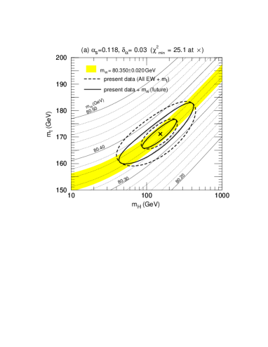
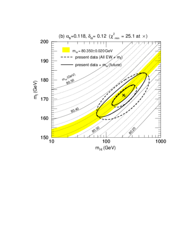
Figure 17: Impact of future improvement in $W$ mass measurement in the ($m_{H},\,m_{t}$) plane, for $\alpha_{s}=0.118$ and $\delta_{\alpha}=0.03$(a), $\delta_{\alpha}=0.12$(b). An assumed future data $m_{W}=80.350\pm 0.020$ is used to constrain $m_{t}$ and $m_{H}$ in addition to the present all electroweak data and the Tevatron $m_{t}$ data, $m_{t}=175\pm 6{\,\rm GeV}$. The inner and outer contours correspond to $\Delta\chi^{2}=1$ ($\sim$ 39% CL), and $\Delta\chi^{2}=4.61$ ($\sim$ 90% CL), respectively. The minimum of $\chi^{2}$ is marked by the sign “$\times$”. Thin dotted/solid lines show the SM predictions for $m_{W}$ when $m_{t}$ and $m_{H}$ are given.

Improved values on the $W$ mass are expected from CDF, D0 at the Tevatron, from the HERA experiments and from the collaborations at LEP2. It is expected to obtain the $W$-mass to 31 MeV for a 1 fb^-1 run at the Tevatron, which may be reduced to 11 MeV for 10 fb^-1[49], while at LEP2 in a 500 pb^-1-run 35 MeV[52] is expected. In a high luminosity run at HERA a precision of 60 MeV is estimated[53]. Further improved measurements on $m_{W}$ may be anticipated at a future linear $e^{+}e^{-}$ collider[54] or at a $\mu^{+}\mu^{-}$ collider[56]. Such measurements will provide a narrow band in the $(m_{H}\,,m_{t})$-plane similar in width and orientation to the present asymmetry band and constitute a crucial piece of information in challenging the validity of the SM.

We show in Fig. 17 the impact of future improvement in $W$ mass measurement in the ($m_{H},\,m_{t}$) plane, for $\alpha_{s}=0.118$ and $\delta_{\alpha}=0.03$(a), $\delta_{\alpha}=0.12$(b). An assumed future value of

$$m_{W}({\,\rm GeV})=80.350\pm 0.020$$ (6.67)

is used to constrain $m_{t}$ and $m_{H}$ in addition to all the present electroweak data and the present Tevatron value for the top quark mass, $m_{t}=175\pm 6{\,\rm GeV}$. The allowed region in the ($m_{H},\,m_{t}$) plane shrinks considerably, but the individual errors of $m_{H}$ and $m_{t}$ remain essentially unaltered as expected from Eq. 6. By comparing the two figures, (a) and (b), the sensitivity of the future constraints to $\bar{\alpha}(m_{Z}^{2})$ can be studied.

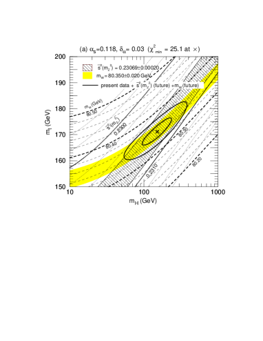
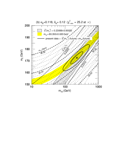
Figure 18: Impact of future improvement in $\bar{s}^{2}(m_{Z}^{2})$ and $W$ mass measurements in the ($m_{H},\,m_{t}$) plane, for $\alpha_{s}=0.118$ and $\delta_{\alpha}=0.03$(a), $\delta_{\alpha}=0.12$(b). Assumed future data $\bar{s}^{2}(m_{Z}^{2})=0.23069\pm 0.00020$ and $m_{W}=80.350\pm 0.020$ are used to constrain $m_{t}$ and $m_{H}$ in addition to the present all electroweak data and the Tevatron $m_{t}$ data, $m_{t}=175\pm 6{\,\rm GeV}$. The inner and outer contours correspond to $\Delta\chi^{2}=1$ ($\sim$ 39% CL), and $\Delta\chi^{2}=4.61$ ($\sim$ 90% CL), respectively. The minimum of $\chi^{2}$ is marked by the sign “$\times$”. Thin dotted/solid lines show the SM predictions for $m_{W}$ when $m_{t}$ and $m_{H}$ are given.

The assumed mean value of $80.350~{}{\,\rm GeV}$ is chosen to retain the $\chi^{2}_{\rm min}$ point of the present data. The effect of changing the average and dispersion of the assumed $m_{W}$ data can be deduced from the two figures.

The precise determinations of both $\bar{s}^{2}(m_{Z}^{2})$ and $m_{W}$ provide independent constraints on $m_{t}$ and $m_{H}$, as can be clearly seen by overlaying Fig. 16 and Fig. 17. Shown in Fig. 18 is the impact of future improvement in $\bar{s}^{2}(m_{Z}^{2})$ and $W$ mass measurements in the ($m_{H},\,m_{t}$) plane, for $\alpha_{s}=0.118$ and $\delta_{\alpha}=0.03$(a), $\delta_{\alpha}=0.12$(b). Assumed future values $\bar{s}^{2}(m_{Z}^{2})=0.23069\pm 0.00020$ and $m_{W}=80.350\pm 0.020$ are shown again by shaded regions. Not only the reduction of the width of the allowed band in the ($m_{H},\,m_{t}$) plane, but also the individual errors of $m_{t}$ and $m_{H}$ are now reduced considerably.

In order to examine the future constraints on ($m_{t}$, $m_{H}$, $\delta_{\alpha}$, $\alpha_{s}$) from the electroweak precision measurements, we repeat the four parameter fit with the present electroweak measurements plus the above two additional ”data” on $\bar{s}^{2}(m_{Z}^{2})$ (6.66) and $m_{W}$ (6.67). We find from the electroweak data only

$$\!\!\left.\begin{array}[]{c@{\,}r@{\,}l}m_{t}({\,\rm GeV})&=&161\pm 5\\[2.84526pt] \mbox{$x_{H}$}&=&-1.24\pm 0.95\\[2.84526pt] \alpha_{s}&=&0.1204\pm 0.0035\\[2.84526pt] \delta_{\alpha}&=&-0.13\pm 0.16\end{array}\right\}\;\rho_{\rm corr}=\left(\begin{array}[]{rrrr}1.00&0.35&-0.10&0.18\\ &1.00&-0.47&-0.80\\ &&1.00&0.42\\ &&&1.00\end{array}\right),\,\,\,\qquad$$ (6.68i)

$$\chi^{2}_{\rm min}/({\rm d.o.f.})=24.6/(23)\,.$$ (6.68j)

By comparing with the present constraints (5.1), we find that the error of $m_{t}$ can be reduced by about a factor of three, that of $x_{H}$, i.e. the logarithm of $m_{H}$ in units of $100{\,\rm GeV}$, and $\delta_{\alpha}$ by a factor of two. It may be worth noting that $m_{t}$ can be predicted to $5~{}{\,\rm GeV}$ accuracy even without assuming external knowledge on $m_{H}$, $\alpha_{s}$, and $\bar{\alpha}(m_{Z}^{2})$.

By imposing the present knowledge of $m_{t}$, $\alpha_{s}$ and $\delta_{\alpha}$, i.e. $m_{t}=175\pm 6{\,\rm GeV}$, $\alpha_{s}=0.118\pm 0.003$ and $\mbox{$\delta_{\alpha}$}=0.03\pm 0.009$, the fit (18) becomes

$$\!\!\left.\begin{array}[]{c@{\,}r@{\,}l}m_{t}({\,\rm GeV})&=&172\pm 6\\[2.84526pt] \mbox{$x_{H}$}&=&0.49\pm 0.60\\[2.84526pt] \alpha_{s}&=&0.1190\pm 0.0022\\[2.84526pt] \delta_{\alpha}&=&0.04\pm 0.08\end{array}\right\}\;\rho_{\rm corr}=\left(\begin{array}[]{rrrr}1.00&0.84&0.13&-0.26\\ &1.00&0.13&-0.63\\ &&1.00&-0.06\\ &&&1.00\end{array}\right),\,\,\,\qquad$$ (6.69i)

$$\chi^{2}_{\rm min}/({\rm d.o.f.})=24.9/(26)\,.$$ (6.69j)

This should be compared with the corresponding result in (13). It is rather surprising to observe that none of the individual errors of the four fitted parameters reduces significantly from the present errors in (13). The mean values stay the same because we chose the mean values of the future $\bar{s}^{2}(m_{Z}^{2})$ and $m_{W}$ data at the present minimum of the global $\chi^{2}$ fit. What did change by adding the above two future ”data” are the correlations among the errors, in particular, that between $m_{t}$ and $\log m_{H}$ is now very large, 0.84, and the negative correlation between $\log m_{H}$ and $\delta_{\alpha}$ has also been strengthened. Therefore, we can expect an important improvement on the $m_{H}$ constraint once $m_{t}$ and $\delta_{\alpha}$ are measured accurately.

6.3 Top-quark mass

It is tantalizing that the present top mass value from Tevatron (5.53) lies just on the boundary of the region allowed by the electroweak data.

The long-range program (TeV33[48, 50]) at the Tevatron envisages an ultimate precision of the top mass of about 2 GeV based on an anticipated yearly integrated luminosity of 10 fb^-1. In the future, the error can be reduced further to 200 MeV at an $e^{+}e^{-}$ LC[55] and possibly down to 70 MeV at a muon collider[56] with precise beam energy resolution. Figure 13 shows us that once the top quark mass is precisely determined, the major remaining uncertainty in electroweak fits is due to $\delta_{\alpha}$, the magnitude of the QED running coupling constant at the $m_{Z}$ scale.

Next we examine the effect of a future measurement $m_{t}=175\pm 2~{}{\,\rm GeV}$ on the four parameter fit (18):

$$\!\!\left.\begin{array}[]{c@{\,}r@{\,}l}m_{t}({\,\rm GeV})&=&175\pm 2\\[2.84526pt] \mbox{$x_{H}$}&=&0.75\pm 0.35\\[2.84526pt] \alpha_{s}&=&0.1192\pm 0.0021\\[2.84526pt] \delta_{\alpha}&=&0.05\pm 0.08\end{array}\right\}\;\rho_{\rm corr}=\left(\begin{array}[]{rrrr}1.00&0.48&0.05&-0.09\\ &1.00&0.07&-0.73\\ &&1.00&-0.03\\ &&&1.00\end{array}\right),\,\,\,\qquad$$ (6.70i)

$$\chi^{2}_{\rm min}/({\rm d.o.f.})=25.2/(26)\,.$$ (6.70j)

The error of the logarithm of $m_{H}$ has been reduced from $\pm 0.60$ (18) to $\pm 0.35$, which is substantial, but not satisfactory. We find that this error cannot be reduced significantly by further reducing the error of $m_{t}$ down to 1 GeV. This may be inferred from the reduced correlation between $m_{t}$ and $\log m_{H}$ in (6.3). The strongest correlation among the four errors now appears between $\log m_{H}$ and $\delta_{\alpha}$. It is clear that further progress about $m_{H}$ in the SM, and also about physics beyond the SM from its quantum effects, will critically depend on an improved determination of $\bar{\alpha}(m_{Z}^{2})$.

As a final example, we present the four parameter fit result with one further constraint, $\mbox{$\delta_{\alpha}$}=0.03\pm 0.03$, where the error is assumed to be 1/3 of the conservative estimate[18], or 1/2 of the other two estimates[16, 17]. We find

$$\!\!\left.\begin{array}[]{c@{\,}r@{\,}l}m_{t}({\,\rm GeV})&=&175\pm 2\\[2.84526pt] \mbox{$x_{H}$}&=&0.69\pm 0.26\\[2.84526pt] \alpha_{s}&=&0.1192\pm 0.0021\\[2.84526pt] \delta_{\alpha}&=&0.03\pm 0.03\end{array}\right\}\;\rho_{\rm corr}=\left(\begin{array}[]{rrrr}1.00&0.58&0.05&-0.04\\ &1.00&0.07&-0.38\\ &&1.00&-0.01\\ &&&1.00\end{array}\right),\,\,\,\qquad$$ (6.71i)

$$\chi^{2}_{\rm min}/({\rm d.o.f.})=25.3/(26)\,.$$ (6.71j)

The error in $\log m_{H}$ is now reduced to about $\pm 0.25$.

To conclude, we examine the constraint on $m_{H}$ from ultimate electroweak measurements by making use of the expressions (6). With the top-quark mass determination of order 100 MeV at a LC or at a muon collider, its error can be safely neglected in (6). Once the $\alpha_{s}$ value is measured to the 1 % level[57], the LEP1 constraint from $\Gamma_{Z}$ becomes more effective through (6.65a). Nevertheless we find that $m_{H}$ will be constrained essentially by the future measurements of $\bar{s}^{2}(m_{Z}^{2})$ and $m_{W}$ within the SM:

$$\Delta\,[\,\mbox{$x_{H}$}-0.44\,x_{\alpha}\,] = \pm\frac{\Delta\bar{s}^{2}(m_{Z}^{2})}{0.0005}\,,$$ (6.72)

$$\Delta\,[\,\mbox{$x_{H}$}-0.20\,x_{\alpha}\,] = \pm\frac{\Delta m_{W}({\,\rm GeV})}{0.06}\,.$$ (6.73)

Combining the above two constraints (6.72) and (6.73) gives

$$\Delta\,[\,\mbox{$x_{H}$}-A\,x_{\alpha}\,] = \pm\sigma\,,$$ (6.74a)

$$\Delta\,x_{\alpha} = \pm\sigma_{\alpha}\,,$$ (6.74b)

with

$$\frac{1}{\sigma^{2}} \approx (\frac{0.0005}{\Delta\bar{s}^{2}(m_{Z}^{2})})^{2}+(\frac{0.06}{\Delta m_{W}})^{2}\,,$$ (6.75a)

$$\frac{A}{\sigma^{2}} \approx 0.44\,(\frac{0.0005}{\Delta\bar{s}^{2}(m_{Z}^{2})})^{2}+0.20\,(\frac{0.06}{\Delta m_{W}})^{2}\,,$$ (6.75b)

$$\frac{1}{\sigma_{\alpha}^{2}} \approx 0.19\,(\frac{0.0005}{\Delta\bar{s}^{2}(m_{Z}^{2})})^{2}+0.04\,(\frac{0.06}{\Delta m_{W}})^{2}-\frac{A^{2}}{\sigma^{2}}+\frac{1}{(\Delta\,x_{\alpha}^{\rm(ext)})^{2}}\,,$$ (6.75c)

where $\Delta\,x_{\alpha}^{\rm(ext)}=\Delta[1/\bar{\alpha}(m_{Z}^{2})]/0.09$ is the external constraint on $\bar{\alpha}(m_{Z}^{2})$. For instance, with $\Delta\bar{s}^{2}(m_{Z}^{2})=0.00010$, $\Delta m_{W}({\,\rm GeV})=0.010$, and $\Delta\,x_{\alpha}^{\rm(ext)}=0.30$, we find $\Delta\,[\,\mbox{$x_{H}$}-0.30\,x_{\alpha}\,]\,=\,\pm 0.13$ with $\Delta\,x_{\alpha}\,=\,\pm 0.29$. Hence with the above ultimate assumptions, the error of the SM prediction to $\log m_{H}$ reduces to $\pm 0.15$. On the other hand, once the Higgs boson is found, its mass may be measured so accurately that its error can be neglected in the electroweak radiative effects. The electroweak data (6.72) and (6.73) then constrain $\delta_{\alpha}$ to $\pm 0.036$, or about 40% its present error[18]. Evidence for new physics may then be looked for by comparing the direct and indirect measurements of $\bar{\alpha}(m_{Z}^{2})$.

6.4 Future constraints on $S$, $T$, $U$

The impact on $S$, $T$, $U$ of the future measurements of $\bar{s}^{2}(m_{Z}^{2})$ (6.66) and $m_{W}$ (6.67) is discussed briefly in this subsection. The analysis of section 4.4 can be repeated straightforwardly.

It is again worth noting that only the following combinations of these parameters and $\delta_{\alpha}$, $\bar{\delta}_{G}$ and $\alpha_{s}$ can be constrained by the three most accurately measurable quantities:

$$\Gamma_{Z}({\,\rm MeV}) \approx 2473.0-9.5\,S^{\prime}+25.0\,T^{\prime}+1.7\,x^{\prime}_{s}-3.4\,\log[\,1+(\frac{26{\,\rm GeV}}{m_{H}})^{2}\,]\,,$$ (6.76a)

$$\bar{s}^{2}(m_{Z}^{2}) \approx 0.2334+0.0036\,S^{\prime}-0.0024\,T^{\prime}$$ (6.76b)

$$m_{W}({\,\rm GeV}) \approx 79.840-0.291\,S^{\prime}+0.417\,T^{\prime}+0.332\,U^{\prime\prime}\,.$$ (6.76c)

Here $x^{\prime}_{s}=(\alpha^{\prime}_{s}-0.118)/0.003=[\alpha_{s}-0.118+1.54\,(\mbox{$\bar{\delta}_{b}$}+0.00995)]/0.003$, and

$$S^{\prime} = S-0.72\,\mbox{$\delta_{\alpha}$}\,,$$ (6.77a)

$$T^{\prime} = T+(0.0055-\bar{\delta}_{G})/\alpha\,,$$ (6.77b)

$$U^{\prime\prime} = U^{\prime}-0.87\,(T^{\prime}-T)$$ (6.77c)

$$= U-0.22\,\mbox{$\delta_{\alpha}$}+0.87\,(0.0055-\bar{\delta}_{G})/\alpha\,.$$

A linear combination of $S^{\prime}$ and $T^{\prime}$ will be better constrained by future improvements in $\bar{s}^{2}(m_{Z}^{2})$. Individual constraints will still be obtained from the LEP1 $\Gamma_{Z}$ value, and hence they won’t be improved significantly unless one can predict accurately the $\alpha_{s}^{\prime}$ value including the $Zb_{L}b_{L}$ vertex factor. The improved measurement on $m_{W}$ determines the combination $U^{\prime\prime}$. Therefore, we need to know $\bar{\delta}_{b}$, $\bar{\delta}_{G}$ and $\delta_{\alpha}$ accurately in order to constrain non-SM contributions to the $S$, $T$, $U$ parameters.

As an example consider the result of the three parameter fit with the new $\bar{s}^{2}(m_{Z}^{2})$ and $m_{W}$ measurements of (6.66) and (6.67), respectively :

$$\!\!\left.\begin{array}[]{c@{}r@{}r@{}r}S^{\prime}=&-0.32&-0.061\,\frac{\alpha_{s}^{\prime}-0.1075}{0.0037}&\pm 0.11\\[2.84526pt] T^{\prime}=&0.61&-0.096\,\frac{\alpha_{s}^{\prime}-0.1075}{0.0037}&\pm 0.14\\[2.84526pt] U^{\prime\prime}=&0.47&+0.065\,\frac{\alpha_{s}^{\prime}-0.1075}{0.0037}&\pm 0.11\\[2.84526pt] \end{array}\right\}\;\rho_{\rm corr}=\left(\begin{array}[]{rrr}1&0.92&-0.60\\[2.84526pt] &1&-0.79\\[2.84526pt] &&1\\[2.84526pt] \end{array}\right),\,\,\,\qquad$$ (6.78g)

$$\chi^{2}_{\rm min}=20.4+\biggl{(}\frac{\alpha_{s}^{\prime}-0.1075}{0.0037}\biggr{)}^{2}+\biggl{(}\frac{\mbox{$\bar{\delta}_{b}$}+0.0051}{0.0028}\biggr{)}^{2}\,,\quad({\rm d.o.f.}=23)\,.$$ (6.78h)

As compared to the present result (8), we find substantial reductions in the error of $U^{\prime\prime}$ but not in those of $S^{\prime}$ and $T^{\prime}$ individually. On the other hand, all correlations are stronger compared to those of Eq. (8). The most stringent constraint among the $S$, $T$, $U$ parameters now reads

$$T^{\prime}-0.96S^{\prime}+0.45U^{\prime\prime}=1.13\pm 0.036.$$ (6.79)

When compared with the corresponding constraint (4.46) of the existing electroweak data, the allowed range of $T^{\prime}$ for given $S^{\prime}$ and $U^{\prime}$ can be reduced by a factor of two.

7 Conclusions

We have carried out a comprehensive analysis of the latest electroweak data. The analysis updates our previous work (see Ref.[2]). The total width $\Gamma_{Z}$, the hadronic width $\Gamma_{h}^{0}$ and the leptonic width $\Gamma_{\ell}$ agree well with the SM predictions at the level of a few $10^{-3}$. The new measurement of $R_{c}$ is in agreement with the SM, and also the new measurement of $R_{b}$, albeit within about two standard deviations. The asymmetry data determine the effective weak mixing parameter $\sin^{2}\theta_{W}$ to an accuracy of 0.1% level, see Eq. (2.2). Their average value agrees well with the SM, while their dispersion is larger than statistically expected. It is, however, fair to conclude that the progress both in precision and agreement of data with SM expectation is impressive.

The ($S$, $T$) fit agrees well with the SM, whereas the simple QCD-like Techni-Color (TC) model is ruled out at the 99%CL. The fitted $U$ parameter also agrees with the SM prediction. The fact that all the $S$, $T$, $U$ parameters agree well with the SM prediction for the top quark mass as observed at the Tevatron and the Higgs boson mass below a few hundred GeV implies that any dynamical model of the electroweak symmetry breaking without a light Higgs boson should not only give a negative $S_{\rm new}$, but also a $T_{\rm new}$-value which is constrained severely by the data for the given $S_{\rm new}$ and $U_{\rm new}$; see Eq. (4.46). The above conclusion remains valid even if the model contributes a sizeable amount to the $Zb_{L}b_{L}$ vertex, since the strong correlation between $S_{\rm new}$ and $T_{\rm new}$ comes from the accurate measurement of the effective weak mixing angle, $\bar{s}^{2}(m_{Z}^{2})$, which is independent of $R_{b}$ or the assumed $\alpha_{s}$ value. For the $U$ parameter, $|U_{\rm new}|\hbox to0.0pt{\lower 3.5pt\hbox{$\mathchar 0\relax\sim$}\hss}\raise 1.0pt\hbox{$<$}0.4$ should be satisfied. The uncertainty in the running QED coupling constant at the $m_{Z}$ scale, $\bar{\alpha}(m_{Z}^{2})$, is shown as the serious limiting factor for future improvements in the determination of the $S$ parameter.

The global fit in the minimal SM in terms of ($m_{t}$, $m_{H}$) yields values for the top mass, $m_{t}=153\pm 10{\,\rm GeV}$ (5.48i), or $m_{t}=158\pm 12{\,\rm GeV}$ (5.50i) if we drop the present $R_{b}$ constraint, which agrees with the direct measurements from the Tevatron, $m_{t}=175\pm 6{\,\rm GeV}$[8]. The corresponding allowed range in $m_{H}$ is $m_{H}=50^{+50}_{-30}{\,\rm GeV}$ (5.48i) and $m_{H}=60^{+100}_{-40}{\,\rm GeV}$ (5.50i) respectively. Once $m_{t}$ is accurately measured the present electroweak data will impose stringent limits on the Higgs-boson mass which are not affected by the $R_{b}$ data (see Table 7 in section 5.2). For instance the present electroweak data favor a light Higgs boson if $m_{t}\hbox to0.0pt{\lower 3.5pt\hbox{$\mathchar 0\relax\sim$}\hss}\raise 1.0pt\hbox{$<$}170{\,\rm GeV}$ while a heavier Higgs boson is favored if $m_{t}\hbox to0.0pt{\lower 3.5pt\hbox{$\mathchar 0\relax\sim$}\hss}\raise 1.0pt\hbox{$>$}180{\,\rm GeV}$: the 95% CL upper and lower mass bounds, $m_{H}<360{\,\rm GeV}$ for $m_{t}=170{\,\rm GeV}$ and $m_{H}>130{\,\rm GeV}$ for $m_{t}=180{\,\rm GeV}$ are obtained by using $\alpha_{s}=0.118\pm 0.003$[28] and $\mbox{$\delta_{\alpha}$}=0.03\pm 0.09$[18]. In order to further improve the constraint on $m_{H}$ not only precise measurement on $m_{t}$ are required, but also improved measurements on $\Delta\alpha_{\rm had}(m_{Z}^{2})$ and $\alpha_{s}$.

For the agreement of the SM predictions with precision experiments it is indispensable to include radiative effects due to ‘vertex-like’ corrections which may be regarded as indirect evidence for the universal weak-boson self-couplings. Their direct investigation will soon be carried out at LEP 2.

Finally, we studied prospects of future improvements in the electroweak precision experiments. Major improvements are expected from further running and detector upgrades in the determination of the mixing parameter $\bar{s}^{2}(m_{Z}^{2})$ at SLC, Tevatron, and at a future linear $e^{+}e^{-}$ collider (LC); $m_{W}$ will be measured more accurately at LEP2, Tevatron upgrades, LHC, LC and, perhaps, at a muon collider. The error in the top-quark mass may be reduced to 2 GeV at Tevatron, 200 MeV at LC, and even further down at a muon collider. These measurements will constrain physics beyond the SM very stringently, say in the $(S_{\rm new},T_{\rm new},U_{\rm new})$ parameter space, where not only $T_{\rm new}$ but also $U_{\rm new}$ will be constrained severely as function of $S_{\rm new}$, whose constraint can be improved with a better $\alpha(m_{Z}^{2})$ knowledge. Within the SM, the constraint on the Higgs boson mass will not improve significantly beyond $\pm 0.35$ for $\log m_{H}$, unless a substantial improvement in the $\alpha(m_{Z}^{2})$ estimate is achieved also.

References

- [1] The LEP Collaborations ALEPH, DELPHI, L3, OPAL, the LEP Electroweak Working Group and the SLD Heavy Flavour Group, preprint CERN-PPE/96-183 (December 1996).
- [2] K. Hagiwara, D. Haidt, C.S. Kim and S. Matsumoto, Z. Phys. C64, 559 (1994); C68 (1995) 352(E).
- [3] S. Matsumoto, Mod. Phys. Lett. A10, 2553 (1995).
- [4] The LEP Collaborations ALEPH, DELPHI, L3, OPAL and the LEP Electroweak Working Group, preprint CERN-PPE/95-172 (1995).
- [5] M.E. Peskin and T. Takeuchi, Phys. Rev. Lett. 65, 964 (1990); Phys. Rev. D46, 381 (1992).
- [6] M. Rijssenbeek, talk at ICHEP96, Warsaw, 25-31 July 1996, Fermilab-Conf-96-365-E, to appear in the proceedings.
- [7] K. McFarland, talk at the XV Workshop on Weak Interactions and Neutrinos, Talloires, France, 4–8 Sep 1995.
-
[8]
CDF Collaboration, J. Lys, talk at ICHEP96, Warsaw, 25-31 July 1996,
Fermilab-Conf-96-409-E, to appear in the proceedings;
D0 Collaboration, S. Protopopescu, talk at ICHEP96, Warwaw, 25-31 July 1996, to appear in the proceedings;
P. Tipton, talk at ICHEP96, Warsaw, 25-31 July 1996, to appear in the proceedings. - [9] K. Hagiwara, Proceedings of 17th International Symposium on Lepton-Photon Interactions(LP95) (Beijing, P.R. China, 10-15 August 1995), p.63.
-
[10]
J.M. Cornwall and J. Papavassiliou, Phys. Rev. D40, 3474 (1989);
J. Papavassiliou and K. Phillippides, ibid.48(1993)4225; ibid.51(1995)6364;
J. Papavassiliou, ibid.50(1994)5998. - [11] G. Degrassi and A. Sirlin, Nucl. Phys. B383, 73 (1992); Phys. Rev. D46, 3104 (1992); G. Degrassi, B. Kniehl and A. Sirlin, ibid.48(1993)R3963.
- [12] D.C. Kennedy and B.W. Lynn, Nucl. Phys. B322, 1 (1989).
- [13] K. Hagiwara, S. Matsumoto and R. Szalapski, Phys. Lett. B357, 411 (1995); K. Hagiwara, T. Hatsukano, R. Ishihara and R. Szalapski, preprint KEK-TH-497, hep-ph/9612268, to appear in Nucl.Phys.B.
- [14] J. Papavassiliou, E. de Rafael and N.J Watson, Preprint CPT-96-P-3408, hep-ph/9612237.
- [15] A. Sirlin, Phys. Rev. D22, 971 (1980).
- [16] A.D. Martin and D. Zeppenfeld, Phys. Lett. B345, 558 (1995).
- [17] M.L. Swartz, Phys. Rev. D53, 5268 (1995).
- [18] S. Eidelman and F. Jegerlehner, Z. Phys. C67, 602 (1995).
- [19] H. Burkhardt and B. Pietrzyk, Phys. Lett. B356, 398 (1995).
- [20] B.A. Kniehl, Nucl. Phys. B347, 86 (1990).
- [21] H. Burkhardt, F. Jegerlehner, G. Penso and C. Verzegnassi, Z. Phys. C43, 497 (1989).
- [22] F. Jegerlehner, in Testing the Standard Model, eds. M. Cvetič and P. Langacker (World Scientific, 1991).
- [23] F. Jegerlehner, cited by B.A. Kniehl in Proc. Europhysics Marseille 1993, p.639.
-
[24]
K.G. Chetyrkin, J.H. Kühn and M. Steinhauser,
Phys. Lett. B351, 331 (1995);
L. Avdeev, J. Fleischer, S. Mikhailov and O. Tarasov, Phys. Lett. B336, 560 (1994); Erratum ibid.349 597 (1995). - [25] K.G. Chetyrkin, J.H. Kühn and M. Steinhauser, Phys. Rev. Lett. 75, 3394 (1995).
- [26] A. Czarnecki and J.H. Kühn, Phys. Rev. Lett. 77, 3955 (1996).
- [27] P.B. Renton, Proceedings of 17th International Symposium on Lepton Photon Interactions (LP95) (Beijing, P.R. China, 10–15 August 1995), p35.
- [28] Particle Data Group, R.M. Barnett et al., Phys. Rev. D54, 1 (1996).
- [29] The OPAL Collaboration, G. Alexander et al., Z. Phys. C72, 1 (1996).
- [30] The OPAL Collaboration, K. Ackerstaff et al., preprint CERN-PPE/96-167 (Nov 1996).
-
[31]
The ALEPH Collaboration,
talk by J.Steinberger in CERN Seminar, : 8 Oct 1996;
The ALEPH Collaboration, R. Barate et al., Preprint CERN-PPE/97-017;
The ALEPH Collaboration, R. Barate et al., Preprint CERN-PPE/97-018. - [32] G.L. Fogli and D. Haidt, Z. Phys. C40, 379 (1988).
- [33] P. Langacker, in Precision Tests of the Standard Electroweak Model, ed. by P. Langacker (World Scientific, 1994).
- [34] T. Appelquist and J. Terning, Phys. Lett. B315, 139 (1993); Phys. Rev. D50, 2116 (1994).
- [35] J. Ellis, G.L. Fogli and E. Lisi, Phys. Lett. B343, 282 (1995).
- [36] G. Altarelli, talk at the NATO Advanced Study Institute on Techniques and Concepts of High Energy Physics, St. Croix, 10–23 July 1996, hep-ph/9611239.
- [37] P. Langacker and J. Erler, presented at the Ringberg Workshop on the Higgs Puzzle, December 1996, hep-ph/9703428.
- [38] J.L. Rosner, hep-ph/9704331, submitted to Comments on Nuclear and Particle Physics.
- [39] J. Ellis, G.L. Fogli and E. Lisi, Phys. Lett. B389, 321 (1996).
- [40] W. de Boer, A. Dabelstein, W. Hollik, W. Mösle and U. Schwickerath, hep-ph/9609209 v4 (Nov, 1996).
- [41] V.A. Novikov, L.B. Okun and M.I. Vysotsky, Mod. Phys. Lett. A8, 2529 (1993); Erratum A8 3301 (1993).
- [42] Y. Okada, M. Yamaguchi, T. Yanagida, Prog. Theor. Phys. 85, 1 (1991); Phys. Lett. B262, 54 (1991); H. Haber, R. Hempfling, Phys. Rev. Lett. 66, 1815 (1991); Phys. Lett. B262, 54 (1991); J. Ellis, G. Ridorfi, F. Zwirner, Phys. Lett. B257, 83 (1991); Phys. Lett. B262, 477 (1991).
- [43] J.D. Bjorken, Phys. Rev. D19, 335 (1978); P.D. Hung and J.J. Sakurai, Nucl. Phys. B143, 81 (1978).
- [44] P. Gambio and A. Sirlin, Phys. Rev. Lett. 73, 621 (1994).
- [45] K. Hagiwara, Proceedings of the International Symposium on Vector Boson Self-Interactions, eds. U. Baur, S. Errede and T. Müller (Los Angeles, 1995, AIP Press), p.185.
- [46] V.A. Novikov, L.B. Okun, A.N. Rozanov and M.I. Vysotsky, Mod. Phys. Lett. A9, 2641 (1994); Z. Hioki, Phys. Lett. B340, 181 (1994).
- [47] P. Rowson, private communication.
- [48] D. Amidei et al., Preprint CDF/DOC/TOP/PUBLIC/3265 (Aug 1995).
- [49] U. Baur and M. Demarteau, Precision electroweak physics at future collider experiments, hep-ph/9611334 v2, to be published in Proceedings of the 1996 DPF/DPB Summer Study on New Directions for High-Energy Physics (Snowmass 96).
- [50] D. Amidei and R. Brock, Future electroweak physics at the Fermilab Tevatron: Report of the TeV2000 Study Group, Fermilab-Pub-96/082 (April 1996).
- [51] T. Omori, Proceedings of the 2’nd Workshop on JLC , ed. by S. Kawabata, KEK Proceedings 91-10, p.315.
- [52] A. Ballestrero et al., Proceedings of the Workshop on Physics at LEP2, G. Altarelli, T. Sjöstrand and F. Zwirner (eds.), CERN Yellow Report CERN 96-01(1996), Vol.1, p.141.
- [53] R.J. Cashmore et al., MPI/PTh/96-105 and Proceedings of the Workshop on future Physics at HERA 1996.
- [54] A. Miyamoto, Physics and Experiments with Linear Colliders, edited by F.A. Harris et al. (World Scientific, 1993), p.141.
- [55] L.H. Orr, Physics and Experiments with Linear Colliders, eds. A.Miyamoto et al. (World Scientific, 1996), p.129.
- [56] V. Barger, M.S. Berger, J.F. Gunion and T. Han, ”Precision -boson and top-quark mass determination at a muon collider”, hep-ph/9702334.
- [57] P.N. Burrows et al., ”Prospects for the precision measurement of ”, hep-ex/9612012, to be published in Proceedings of the 1996 DPF/DPB Summer Study on New Directions for High-Energy Physics (Snowmass 96).