Complete ${\cal O}(\alpha_{s}^{2})$ Corrections to Zero-Recoil Sum Rules for $B\to D^{*}$ Transitions

Abstract

We present the complete ${\cal O}(\alpha_{s}^{2})$ corrections to the Wilson coefficient of the unit operator in the zero-recoil sum rule for the $B\to D^{*}$ transition. We include both perturbative and power-suppressed nonperturbative effects in a manner consistent with the operator product expansion. The impact of these corrections on $|V_{cb}|$ extracted from semileptonic $B\rightarrow D^{*}$ decays near zero recoil is discussed. The mixing of the heavy quark kinetic operator with the unit operator at the two loop level is obtained. ${\cal O}(\alpha_{s})$ corrections to a number of power-suppressed operators are calculated.

I Introduction

Semileptonic decays of $B$ mesons provide an opportunity to measure the Cabibbo-Kobayashi-Maskawa matrix parameter $|V_{cb}|$ with minimal theoretical uncertainties (for a recent review, see e.g. [1]). One of the two most popular methods is based on the experimental determination of the zero-recoil $B\rightarrow D^{*}$ transition amplitude by extrapolating the experimental decay rate of $B\rightarrow D^{*}\,\ell\nu$ to the point of zero recoil momentum, where the invariant mass squared of leptons is $q^{2}_{\ell\nu}=(M_{B}-M_{D^{*}})^{2}$. The hadronic $B\rightarrow D^{*}$ transition amplitude for this kinematics is written as:

$$\langle{D^{*}}|{\bar{c}\gamma_{\mu}\gamma_{5}b}|{B}\rangle\;=\;2\,F_{D^{*}}\sqrt{M_{B}M_{D^{*}}}\;e^{*}_{\mu}\;,$$ (1)

where $e$ is the polarization vector of the $D^{*}$ meson. The zero-recoil form factor $F_{D^{*}}$ is calculable in the short-distance perturbative expansion up to terms $\sim(\Lambda_{\rm QCD}/m_{c,b})^{2}$. These nonperturbative corrections cannot be evaluated in a model-independent way at present; they are expected to be about $-8\%$ [1].

Existing estimates of the long-distance strong interaction corrections to $F_{D^{*}}$ are based on the sum rules for heavy flavor transitions [2, 3]. They relate certain sums of the transition probabilities to expectation values of local heavy quark operators in the decaying hadron. The zero-recoil sum rule for the spatial components of the axial current can be written in the form:

$$|F_{D^{*}}|^{2}+\sum_{\epsilon<\mu}\,|F_{\rm exc}|^{2}\;=\;\xi_{A}(\mu)\;-\;\frac{\xi_{\pi}(\mu)}{m_{c}^{2}}\mu_{\pi}^{2}(\mu)\;-\;\frac{\xi_{G}(\mu)}{m_{c}^{2}}\mu_{G}^{2}(\mu)\;+\;{\cal O}\left(\frac{\mu^{3}}{m_{Q}^{3}}\right)\;.$$ (2)

The functions $\xi_{A}$, $\xi_{\pi}$ and $\xi_{G}$ are short-distance (perturbative) coefficient functions, $m_{Q}$ denotes heavy quark masses $m_{b,c}$ and $\mu_{\pi}^{2}$, $\mu_{G}^{2}$ are $B$-meson expectation values of the kinetic and chromomagnetic operators, respectively:

$$\mu_{\pi}^{2}(\mu)=\frac{1}{2M_{B}}\langle{B}|{\bar{b}(i\vec{D})^{\,2}b}|{B}\rangle_{\mu}\;,\;\;\;\;\mu_{G}^{2}(\mu)=\frac{1}{2M_{B}}\langle{B}|{\bar{b}\frac{i}{2}\sigma_{\alpha\beta}G^{\alpha\beta}b}|{B}\rangle_{\mu}\;.$$ (3)

By $F_{\rm exc}\,$ we generically denote transition form factors between $B$ and excited charm states with masses $M_{D}+\epsilon$. They are related to the appropriate structure function of the $B$ meson:

$$|F_{D^{*}}|^{2}+\sum_{\epsilon<\mu}\,|F_{\rm exc}|^{2} = \frac{1}{2\pi}\,\int_{0}^{\mu}w_{1}^{A}(\epsilon\,,\vec{q}=0)\,{\rm d}\epsilon\;,$$ (4)

$$w_{1}^{A} = \frac{2}{3}\,{\rm Im}\,h_{ii}^{A}\qquad\epsilon=M_{B}-M_{D^{*}}-q_{0}\;\;,$$ (5)

with the invariant hadronic amplitudes $h$ defined as in [3]:

$$\hat{T}_{\mu\nu} = i\int{\rm d}^{4}x{\rm e}\,^{-iqx}\>{\rm T}\left\{j^{\dagger}_{\mu}(x)\,j_{\nu}(0)\right\}\qquad(\mbox{here }j_{\mu}=\bar{c}\gamma_{\mu}\gamma_{5}b),$$ (6)

$$h^{A}_{\mu\nu} \equiv {1\over 2M_{B}}\langle B|\hat{T}_{\mu\nu}|B\rangle.$$ (7)

The derivation of such sum rules and their usage for estimating physical form factors is explained in detail in [3].

Because of short-distance perturbative effects the sum over excited states in the l.h.s. of the sum rules does not converge at $\epsilon\sim\Lambda_{\rm QCD}$. Instead, for $\Lambda_{\rm QCD}<\epsilon<m_{Q}$ one has $w_{1}^{A}(\epsilon\,,\vec{q}=0)\sim\alpha_{s}(\epsilon)\epsilon/m_{Q}^{2}$. This necessitates introducing a cutoff at some energy $\mu$. The cutoff serves as a natural normalization point of the effective low-energy operators, most appropriate for use with the sum rules. The scale $\mu$ satisfies the constraint $\Lambda_{\rm QCD}\ll\mu\ll m_{c,b}$. As explicitly indicated in Eq. (2), all coefficient functions are also $\mu$-dependent.

The leading term $\xi_{A}(\mu)$ is of primary importance, since it accounts for the short-distance perturbative renormalization of the zero-recoil axial current. It is calculable in the perturbative expansion provided $\mu$ is large enough and belongs to the perturbative domain. If $\mu$ is too large, it weakens the constraining power of the sum rules, since the heavy quark expansion runs in powers of $\mu/m_{Q}$.

The ${\cal O}(\alpha_{s})$ perturbative corrections to the sum rules were calculated in [3] (see also [4]). Separate pieces of BLM–corrections [5] contributing to sum rules at order ${\cal O}(\beta_{0}\alpha_{s}^{2})$ were considered in [6, 7, 8]. The complete BLM resummation of the unit operator coefficient function $\xi_{A}(\mu)$ was carried out in [9]. The impact of these quasi–one-loop corrections on the sum rules proved to be small when one follows the Wilson approach to the Operator Product Expansion (OPE) assuming explicit separation of short-distance and long-distance contributions.

More challenging are the genuine, non-BLM ${\cal O}(\alpha_{s}^{2})$ corrections. Their magnitude is crucial for estimating the actual impact of unknown higher-order corrections. Technically the most complicated piece corresponding to virtual corrections to heavy quark currents at zero recoil was calculated to order ${\cal O}(\alpha_{s}^{2})$ in [10]. In the present paper the remaining second-order corrections to the zero-recoil sum rule for spatial components of the axial current are computed and the complete two-loop expression for the perturbative coefficient function $\xi_{A}(\mu)$ is given. We also derive the two-loop evolution of the kinetic operator. As a byproduct of the analysis, we find ${\cal O}(\alpha_{s})$ corrections to coefficients of some power suppressed operators in the nonrelativistic expansion, and obtain a similar correction to the coefficient of the kinetic operator in the sum rule. The ${\cal O}(\alpha_{s}^{2})$ correction to the sum rule for the timelike component of the vector current ($B\rightarrow D$ transition) will be given elsewhere.

II ${\cal O}(\alpha_{s}^{2})$ corrections to $\xi_{A}(\mu)$

The most efficient way to determine $\xi_{A}(\mu)$ was suggested in [3] (see also [11, 9]). It relies on considering the OPE relations of the type of Eq. (2) in perturbation theory. The structure function $w_{A}$ is then given by the weak transitions amplitudes between initial and final states consisting of quarks and gluons. Our aim here is to calculate it to order ${\cal O}(\alpha_{s}^{2})$.

The l.h.s. has an elastic contribution $b\rightarrow c$ for on-shell quarks and the continuum contribution from $b\rightarrow c+{\rm gluon}$ and $b\rightarrow c+{\rm 2\>gluons}$. The elastic contribution is equal to $|\eta_{A}^{(2\,\rm loop)}|^{2}$, which was calculated in [10]. The inelastic part of the structure function to order ${\cal O}(\alpha_{s}^{2})$ is calculated in the present paper as an expansion in $\mu/m_{Q}$. In order to determine perturbative coefficients in the sum rules, we need the inelastic part only through the leading, second order in $\mu/m_{Q}$, because as far as nonperturbative effects emerging from local higher-dimension operators are concerned, we account explicitly only for $1/m_{Q}^{2}$ terms.

Therefore, in order to calculate $\xi_{A}(\mu)$ with ${\cal O}(\alpha_{s}^{2})$ accuracy, one has to calculate $\eta_{A}^{2}$, the inelastic part of the structure function $w_{1}^{A}$, the perturbative correction to the coefficient function $\xi_{\pi}(\mu)$ of the kinetic operator and the perturbative expectation value of the kinetic operator to the necessary order in $\alpha_{s}$. The expectation value of the chromomagnetic operator vanishes in the perturbative expansion to leading order in $1/m_{Q}$.

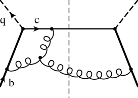
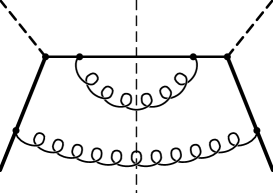
Through order $\alpha_{s}^{2}\mu^{2}/m_{Q}^{2}$ the perturbative contribution to the l.h.s. of Eqs. (2), (4) has the form (the Feynman diagrams for the inelastic part are shown in Fig. 1):

$$\frac{1}{2\pi}\,\int_{0}^{\mu}w_{1}^{A\,({\rm pert})}(\epsilon\,,0)\,{\rm d}\epsilon\;=\;\left(\eta_{A}^{(\rm 2\,loop)}\right)^{2}+\left\{\frac{\alpha_{s}(M)}{\pi}C_{F}\Delta_{1}^{A}+\Bigg{(}\frac{\alpha_{s}}{\pi}\Bigg{)}^{2}C_{F}\Delta_{2}^{A}(\mu;\,M)\right\}\left(\frac{\mu}{m_{c}}\right)^{2},$$ (8)

where $M$ is a normalization point for the strong coupling constant in the $\overline{\rm MS}$ scheme. Denoting $x=m_{c}/m_{b}$, we get:

$$\Delta_{1}^{A}=\frac{1}{4}\Bigg{(}1+\frac{2}{3}x+x^{2}\Bigg{)},$$ (9)

$$\Delta_{2}^{A}=C_{F}\Delta_{F}^{A}+C_{A}\Delta_{A}^{A}+T_{R}N_{L}\Delta_{L}^{A},$$ (10)

$$\Delta_{F}^{A}(\mu) = \ln\left(x\right)\left(-{2\over 1-x}+{13\over 8}+x+{3\over 8}x^{2}\right)-{25\over 36}-{11\over 18}x-{25\over 36}x^{2},$$ (11)

$$\Delta_{A}^{A}(\mu) = \ln\left(x\right)\left(-{1\over 4}-{1\over 12}x\right)+\Delta_{1}^{A}\left[\ln\left(\frac{2\mu}{m_{c}}\right)-{5\over 24}\pi^{2}+{11\over 6}\ln\left(\frac{M}{2\mu}\right)\right]$$ (13)

$$\quad+{917\over 720}+{949\over 1080}x+{917\over 720}x^{2},$$

$$\Delta_{L}^{A}(\mu) = -{77\over 180}-{89\over 270}x-{77\over 180}x^{2}-\frac{2}{3}\,\Delta_{1}^{A}\ln\left(\frac{M}{2\mu}\right).$$ (14)

Although the sum of the elastic $b\rightarrow c$ transition probability and the inelastic excitations is more infrared-stable than they are separately, it is still not completely free of power suppressed infrared contributions. Its infrared part is given by the expectation values of the local operators in the r.h.s. of the sum rule (2). Therefore, by calculating the expectation values of the local operators in perturbation theory and accounting for them in Eq.(2), we eliminate the contribution of the infrared domain from the Wilson coefficient of the unit operator $\xi_{A}(\mu)$.

The expectation value of the kinetic operator in perturbation theory can be determined by using the sum rule for spatial components of the vector current at zero recoil in the heavy quark limit [2, 3, 9]:

$$\frac{1}{2\pi}\,\int_{0}^{\mu}w_{1}^{V}(\epsilon)\,{\rm d}\epsilon\;=\;\frac{\xi^{V}_{\pi}}{m_{c}^{2}}\mu_{\pi}^{2}(\mu)\;-\;\frac{\xi^{V}_{G}(\mu)}{m_{c}^{2}}\mu_{G}^{2}(\mu)\;\;.$$ (15)

The excitation probability (the perturbative structure function) $w_{1}^{V}(\epsilon)$ is calculated using the same technique as for the axial current. To apply this sum rule, however, we need the coefficient functions $\xi^{V}_{\pi}$ with ${\cal O}(\alpha_{s})$ accuracy. For this purpose we perform a nonrelativistic expansion of the vector current accounting for the ${\cal O}(\alpha_{s})$ corrections. The result of this calculation reads:

$$\bar{c}\vec{\gamma}b\;|_{\vec{q}=0} = \varphi_{c}^{+}\left(-u\,i\vec{D}\;+\;v\,[\vec{\sigma}\times\vec{D}]\right)\varphi_{b}\;,$$ (16)

$$u = {1\over m_{b}}\left\{{1+x\over 2x}\left[1-C_{F}\frac{\alpha_{s}}{\pi}\left(\frac{3(1+x)}{4(1-x)}\ln(x)+1\right)\right]\;+\;C_{F}\frac{\alpha_{s}}{2\pi}\frac{\ln(x)}{1-x}\;\right\},$$ (17)

$$v = {1\over m_{b}}{1-x\over 2x}\left[1-C_{F}\frac{\alpha_{s}}{\pi}\left(\frac{3(1+x)}{4(1-x)}\ln(x)+1\right)\right].$$ (18)

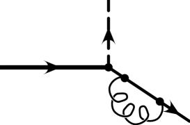
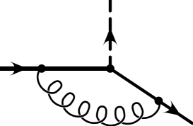
This is the ${\cal O}(\alpha_{s})$–corrected form of the expansion for the vector current given in [3], Eq. (181). The coefficients $u$ and $v$ are obtained by evaluating one-loop graphs shown in Fig. 2 in the linear approximation in $\vec{p}_{b,c}/m_{Q}$. Using Eqs. (16) one determines the normalization of the state produced by the vector current:

$$\frac{1}{3}\sum_{n}|\langle{n}|{\bar{c}\gamma_{i}b}|{B}\rangle|^{2}\;=\;\frac{1}{3}\left[(u^{2}+2v^{2})\,\mu_{\pi}^{2}\;-\;(v^{2}-2uv)\,\mu_{G}^{2}\right]\;.$$ (19)

As was shown in Ref. [3], this normalization is nothing but the sum rule of interest. We get

$$\xi^{V}_{\pi} = \frac{1}{4}\left\{\left(1-\frac{2}{3}x+x^{2}\right)-2C_{F}\frac{\alpha_{s}}{\pi}\left[\left(1-\frac{2}{3}x+x^{2}\right)+\frac{3}{4}\frac{1+x}{1-x}\ln{x}\left(1-\frac{10}{9}x+x^{2}\right)\right]\right\},$$ (20)

$$\xi^{V}_{G} = \frac{1}{4}\left\{\left(-\frac{1}{3}-\frac{2}{3}x+x^{2}\right)-2C_{F}\frac{\alpha_{s}}{\pi}\left[\left(-\frac{1}{3}-\frac{2}{3}x+x^{2}\right)-\ln x\left(\frac{1}{4}+\frac{2}{3}x+\frac{3}{4}x^{2}\right)\right]\right\}\,.$$ (21)

The same expression for $\xi_{\pi}^{V}$ can be also obtained by considering the sum rule for a slowly moving $b$ quark. Below, this method is applied to derive the Wilson coefficient of the kinetic operator $\xi_{\pi}$ which enters the axial sum rule [cf. Eqs. (24)–(26)].

In order to get the expectation value of the kinetic operator in perturbation theory and, therefore, its mixing with the unit operator to ${\cal O}(\alpha_{s}^{2})$ accuracy, one has to evaluate the l.h.s. of the sum rule (15) to second order in perturbation theory through terms $\mu^{2}/m_{Q}^{2}$. Since the chromomagnetic operator does not mix with the unit operator, the perturbative contribution as a whole should be identified with the kinetic operator.

Performing this calculation, we get, with the ${\cal O}(\alpha_{s}^{2})$ accuracy:

$$\left(\mu_{\pi}^{2}(\mu)\right)_{\rm pert}\;=\;C_{F}\,\frac{\alpha_{s}(2\mu)}{\pi}\>\mu^{2}\;+\;C_{F}\,\left(\frac{\alpha_{s}}{\pi}\right)^{2}\,\left[\left(\frac{91}{18}-\frac{\pi^{2}}{6}\right)C_{A}-\frac{13}{9}T_{R}N_{L}\right]\>\mu^{2}\;,$$ (22)

$$\frac{{\rm d}\mu_{\pi}^{2}(\mu)}{{\rm d}\mu^{2}}=C_{F}\frac{\alpha_{s}(\mu)}{\pi}+\left(\frac{5}{3}-\ln{2}\right)C_{F}\left(\frac{11}{6}C_{A}-\frac{2}{3}T_{R}N_{L}\right)\left(\frac{\alpha_{s}}{\pi}\right)^{2}+\left(\frac{13}{12}-\frac{\pi^{2}}{6}\right)C_{A}C_{F}\left(\frac{\alpha_{s}}{\pi}\right)^{2}.$$ (23)

The last term in Eq. (23) represents the non-BLM contribution. Note that the term $\sim C_{F}^{2}$ is absent. It means that the first-order mixing in the Abelian theory without light flavors is not renormalized by effects of higher orders. We note that this fact actually holds to all orders in perturbation theory (see Ref. [9]).

Finally, we calculate the coefficient function $\xi_{\pi}(\mu)$ of the kinetic operator in the axial sum rule Eq. (2) to order ${\cal O}(\alpha_{s})$. The result is as follows:

$$\xi_{\pi}(\mu) = \xi_{\pi}^{(0)}\,+\,C_{F}\frac{\alpha_{s}}{\pi}\xi_{\pi}^{(1)}(\mu)\,+\,{\cal O}\left(\frac{\mu}{m_{Q}}\alpha_{s},\,\alpha_{s}^{2}\right)\>,\qquad\qquad$$ (24)

$$\xi_{\pi}^{(0)} = \frac{1}{4}\left(1+\frac{2}{3}x+x^{2}\right),$$ (25)

$$\xi_{\pi}^{(1)}(\mu) = \frac{2}{3}(1-x)^{2}\ln\left(\frac{2\mu}{m_{c}}\right)+\frac{9-17x+31x^{2}-7x^{3}}{24(1-x)}\ln x+\frac{1+22x+x^{2}}{18}.$$ (26)

The last relation is obtained by considering the zero-recoil sum rule perturbatively, in the first order in $\alpha_{s}$ for the initial $b$ quark moving with spatial momentum $|\vec{p}\,|\ll m_{b},~{}m_{c}$. Let us note that for $m_{b}\neq m_{c}$, the zero recoil condition $\vec{q}=0$ implies a change in the spatial quark velocity. This change leads to gluon bremsstrahlung. The virtual corrections become infrared divergent, this divergence, as usual, is compensated by the contribution of the real gluon emission. This cancelation, however, brings in an explicit logarithmic dependence of $\xi_{\pi}^{(1)}$ on $\mu$.

We note that this logarithmic dependence is not quite usual. Although the kinetic operator has a vanishing anomalous dimension, its coefficient in the sum rule contains the logarithm of the cut-off parameter $\mu$ at order $\alpha_{s}$. Because of the power mixing of the kinetic operator with the unit operator, the coefficient of the latter has a similar logarithm in the power suppressed term $\alpha_{s}^{2}\mu^{2}/m_{Q}^{2}$. We must emphasize, however, that the $\log\mu$ in Eq. (26) does not originate from the dependence of the coefficient function on the normalization point used for the kinetic operator, but rather from the explicit dependence of the observable we consider (axial sum rule) on $\mu$. If we introduce a normalization point $\nu$ of the operator as an independent parameter not equal to $\mu$, there will be no $\log\nu$ dependence in $\xi_{\pi}^{1}$ and only $\alpha_{s}\log\mu$ will remain. A transparent physical picture underlying this fact will be discussed in a separate publication.

Equations (8), (22) and (24)–(26) combined with the known result for $\eta_{A}^{(2\,\rm loop)}$ allow us to obtain $\xi_{A}$ to order $\alpha_{s}^{2}$. We note, however, that our perturbative expressions were given in terms of the pole masses of the heavy quarks as they appear in this order of perturbation theory. To get rid of spurious $1/m_{Q}$ infrared effects associated with the pole masses, we have to switch to the short-distance masses $m_{b,c}(\mu)$ which have concrete numerical values at a given $\mu$, independent of the order of perturbation theory. To order $1/m_{Q}^{2}$ this change affects only the term $\eta_{A}^{2}$. Unless this is done, the sum rules are formally inconsistent since the perturbative expansion of $\eta_{A}$ has an infrared piece of the order of $\alpha_{s}(m_{Q})\Lambda_{\rm QCD}/m_{Q}$ [11].

In principle, the short-distance masses can be defined in different ways. Since throughout this paper the renormalization scheme with the cutoff over the excitation energy is implemented, we use the ${\cal O}(\alpha_{s})$ relation [12]

$$\frac{{\rm d}m_{Q}(\mu)}{{\rm d}\mu}\;=\;-C_{F}\frac{\alpha_{s}}{\pi}\left(\frac{4}{3}+\frac{\mu}{m_{Q}}+{\cal O}\left(\frac{\mu^{2}}{m_{Q}^{2}}\right)\,\right)\;.$$ (27)

Then we replace

$$|\eta_{A}^{(2\,{\rm loop})}\left(m_{Q}^{\rm pole}\right)|^{2}\;\rightarrow\;|\eta_{A}^{(2\,{\rm loop})}\left(m_{Q}(\mu)\right)|^{2}$$ (29)

$$\qquad\qquad-\;2C_{F}^{2}\left(\frac{\alpha_{s}}{\pi}\right)^{2}\,\left(\frac{2x}{1-x}\ln x+1+x\right)\;\left(\frac{\mu}{m_{c}}+\frac{3}{8}(1+x)\left(\frac{\mu}{m_{c}}\right)^{2}\right)\;.$$

The final result for the coefficient function $\xi_{A}(\mu)$ of the unit operator is obtained by combining all terms calculated above. Following [13], we express the result in terms of $\alpha_{s}\left(\sqrt{m_{c}m_{b}}\right)$, even though the $m_{c}\leftrightarrow m_{b}$ symmetry arguments (which motivate this choice) do not apply for $\xi_{A}(\mu)$ because an additional momentum scale is present.

Collecting all pieces together and neglecting terms $\mu^{3}/m_{Q}^{3}$, we obtain for $\xi_{A}(\mu)$:

$$\xi_{A}^{(2\,\rm{loop})}(\mu) = \left(\eta_{A}^{(2\,\rm{loop})}(m_{Q}(\mu))\right)^{2}+C_{F}\frac{\alpha_{s}}{\pi}\xi_{A}^{(1)}\left(\frac{\mu}{m_{c}}\right)^{2}$$ (31)

$$+\;C_{F}^{2}\left(\frac{\alpha_{s}}{\pi}\right)^{2}\frac{\mu}{m_{c}}\varsigma_{A}\;+\;C_{F}\left(\frac{\alpha_{s}}{\pi}\right)^{2}\left(\frac{\mu}{m_{c}}\right)^{2}\zeta_{A}^{(2)}\;,$$

$$\varsigma_{A} = -2\left(\frac{2x}{1-x}\ln x+1+x\right),$$ (32)

$$\zeta_{A}^{(2)} = C_{F}\zeta_{A}^{F}+C_{A}\zeta_{A}^{A}+T_{R}N_{L}\zeta_{A}^{L},$$ (33)

$$\zeta_{A}^{F} = \frac{2}{3}(1-x)^{2}\ln\left(\frac{2\mu}{m_{c}}\right)-\frac{x(17+5x+4x^{2})}{6(1-x)}\ln x-\frac{25}{18}-\frac{8}{9}x-\frac{25}{18}x^{2},$$ (34)

$$\zeta_{A}^{A} = -\left(1+\frac{2x}{3}+x^{2}\right)\left[\frac{2}{3}\ln\left(\frac{2\mu}{m_{c}}\right)+\frac{3\pi^{2}}{32}\right]\;$$ (36)

$$-\;\left(\frac{17}{24}+\frac{7x}{18}+\frac{11x^{2}}{24}\right)\ln x+\frac{203}{80}+\frac{1859}{1080}x+\frac{203}{80}x^{2},$$

$$\zeta_{A}^{L} = \frac{1}{3}\left(1+\frac{2x}{3}+x^{2}\right)\left[\ln\left(\frac{2\mu}{m_{c}}\right)+{1\over 2}\ln x\right]-\frac{71}{90}-\frac{77x}{135}-\frac{71x^{2}}{90}.$$ (37)

The function $\eta_{A}^{(2\,\rm{loop})}$ to order ${\cal O}(\alpha_{s}^{2})$ can be found in [10].

Since the BLM part of the corrections was discussed in the literature in detail [9], we single out the genuine non-BLM part $a_{2}^{0}$ which is defined as the value of the full second-order coefficient $a_{2}$ at $N_{L}=\frac{11}{4}\frac{C_{A}}{T_{R}}\>$:

$$\xi_{A}(\mu) = 1\,+\,a_{1}\left(\mu,\,m_{Q}(\mu)\right)\frac{\alpha_{s}}{\pi}\;+\;a_{2}\left(\mu,\,m_{Q}(\mu)\right)\left(\frac{\alpha_{s}}{\pi}\right)^{2}\;+\;...$$ (38)

$$= \;1+a_{1}\left(\mu,\,m_{Q}(\mu)\right)\frac{\alpha_{s}}{\pi}\;+\left[c_{2}^{\rm BLM}\left(\mu,m_{Q}(\mu)\right)\beta_{0}+a_{2}^{0}\left(\mu,m_{Q}(\mu)\right)\right]\left(\frac{\alpha_{s}}{\pi}\right)^{2}+...\;,$$ (39)

$$\beta_{0} = \frac{11}{3}C_{A}-\frac{4}{3}T_{R}N_{L}\;.$$ (40)

Note that $a_{2}^{0}$ does not depend on the convention for the normalization point of the strong coupling. Its value is shown in Fig. 3 as a function of $\mu/m_{c}$ for three values of $m_{c}/m_{b}\;=\;0.2,\;0.25$ and $0.3$. We denote the corresponding non-BLM second-order shift in $\xi_{A}(\mu)$ by $\Delta^{0}(\mu)$:

$$\Delta^{0}(\mu)\;=\;a_{2}^{0}\left(\mu,\,m_{Q}(\mu)\right)\left(\frac{\alpha_{s}}{\pi}\right)^{2}\;.$$

III $|V_{cb}|$ determination and zero–recoil sum rules

Let us now turn to the application of our results for the determination of $|V_{cb}|$. First, we note that the net impact of the non-BLM $\alpha_{s}^{2}$ corrections on the sum rules is rather small. Taking a reasonable value $\mu/m_{c}=0.5$ and $m_{c}/m_{b}=0.25$ we get $a_{2}^{0}\approx-0.7$. Assuming $\alpha_{s}=0.22$ to $0.27$, the absolute shift $\Delta^{0}(\mu)$ constitutes $-0.003$ to $-0.005$ which translates into $-0.0015$ to $-0.0025$ decrease of the short-distance perturbative renormalization of the zero-recoil axial current. For any reasonable choice of the parameter $\mu$ in the sum rules consistent with using the $1/m_{c}$ expansion, this effect is well below 1%. It should be noted that since in the Wilson OPE the infrared domain is completely excluded from the coefficient functions, the effective coupling cannot become large.

The perturbative correction to the coefficient of the kinetic operator (Eq. (26)) is strongly suppressed. The actual value of this coefficient changes only by several percent. We did not calculate the corresponding effect in the chromomagnetic term; due to the anomalous dimension of this operator it depends on the specific renormalization procedure. In view of the result for the vector sum rule (see Eq. (21)) we do not expect this correction to be significant either.

The axial sum rule (2) allows one to get a QCD-based estimate of the combined effect of the perturbative and nonperturbative effects on the $B\rightarrow D^{*}$ zero-recoil form factor:

$$|F_{D^{*}}|=\left[\xi_{A}(\mu)-\frac{\xi_{\pi}(\mu)}{m_{c}^{2}}\mu_{\pi}^{2}(\mu)-\frac{\xi_{G}(\mu)}{m_{c}^{2}}\mu_{G}^{2}(\mu)-\sum_{\epsilon<\mu}\,|F_{\rm exc}|^{2}\right]^{1/2}+\;{\cal O}\left(\frac{\mu^{3}}{m_{Q}^{3}}\right)\;.$$ (41)

It is seen that $\sqrt{\xi_{A}(\mu)}$ plays the role of a short-distance renormalization factor of the weak current, while the remaining terms in square brackets yield $1/m^{2}$ long-distance corrections to the form factor. The quantum-mechanical meaning of each of the three power terms, confirming this formal conclusion, was elucidated in [3] (see also [1]).

With the good perturbative control over the short-distance part of $F_{D^{*}}$, the main uncertainty dominating theoretical predictions for the form factor resides in power corrections.

In Ref. [9] higher order BLM–type corrections to the sum rule were analyzed. It was shown that, assuming that the running of the QCD coupling $\alpha_{s}$ below the charm mass is a valid practical concept, it is necessary to perform a resummation of the leading BLM corrections in order to arrive at a meaningful numerical result. Within the Wilson approach to OPE, the overall impact of the BLM corrections appears to be moderate. The typical BLM-resummed value for $\xi_{A}(\mu)$ at $\mu/m_{c}\simeq 0.5$ appears to be near $0.99$.

On the practical side, excluding the infrared domain notably improves the accuracy of the perturbative calculations for the charm quark, at least in the context of the BLM calculus. We recall that the perturbative zero-recoil factor $\eta_{A}$ has an intrinsic uncertainty $\sim(\Lambda_{\rm QCD}/m_{c})^{2}$ due to infrared renormalons. By calculating $|\xi_{A}(\mu)|^{1/2}$ and taking into account $\mu^{2}/m_{Q}^{2}$ terms, the $(\Lambda_{\rm QCD}/m_{c})^{2}$ uncertainty $\delta_{\rm IR}^{1/m^{2}}$ is eliminated. As long as we do not account for $1/m_{Q}^{3}$ terms explicitly, the perturbative expressions still have an infrared renormalon uncertainty of the order of $(\Lambda_{\rm QCD}/m_{c})^{3}$. Using the same overall normalization for both cases one has

$$\delta_{\rm IR}^{1/m^{2}}(\eta_{A})\>\sim\>(1+x)^{2}\left(\frac{\Lambda_{\rm QCD}}{m_{c}}\right)^{2}\;\rightarrow\;\>\delta_{\rm IR}^{1/m^{3}}\>\sim\>\frac{3{\rm e}^{5/6}}{16}(11+5x+5x^{2}+11x^{3})\left(\frac{\Lambda_{\rm QCD}}{m_{c}}\right)^{3}.$$ (42)

Performing a simple estimate, one finds that the size of the $1/m_{c}^{2}$ uncertainty in $\eta_{A}$ becomes quite significant for $\Lambda_{\rm QCD}\simeq 250\,\mbox{MeV}$. This shows up in the BLM corrections which become quite large already at the lowest orders. Shifting the uncertainty down to $\sim(\Lambda_{\rm QCD}/m_{c})^{3}$, we significantly reduce it.

The analysis of the ${\cal O}(\alpha_{s}^{2})$ corrections presented in this paper shows that the genuine two-loop effects are quite small. Therefore, our numerical conclusions do not differ in practice from the estimate of the zero-recoil axial form factor given in [1]

$$F_{D^{*}}\;\simeq\;0.91\;-\;0.013\,\frac{\mu_{\pi}^{2}-0.5\,\mbox{GeV}^{2}}{0.1\,\mbox{GeV}^{2}}\;\pm\;0.02_{\rm excit}\;\pm\;0.01_{\rm pert}\;\pm\;0.025_{1/m^{3}}\;\;.$$ (43)

For further improvements, one has to bring in a new dynamical input yielding the magnitude of long-distance $1/m_{c}^{2}$ and $1/m_{c}^{3}$ corrections more precisely.

Experimental data on the small-recoil $B\rightarrow D^{*}$ decay rate are not fully conclusive yet. Nevertheless, the value of $|V_{cb}|$ extracted from the exclusive $B\rightarrow D^{*}$ transitions using $F_{D^{*}}\simeq 0.9$ seems to be in a reasonable agreement — already within experimental uncertainties — with the results obtained from inclusive semileptonic decay width $\Gamma_{\rm sl}(B\to X_{c}l\nu_{l})$. The estimate of the complete ${\cal O}(\alpha_{s}^{2})$ correction in $\Gamma_{\rm sl}(b\rightarrow X_{c}l\nu_{l})$, recently presented in Ref. [14], is another example of the theoretical progress in the perturbative treatment of one of the most important heavy quark decays.

IV Conclusions

We have calculated the complete ${\cal O}(\alpha_{s}^{2})$ corrections to the zero-recoil heavy quark axial sum rule which is used to evaluate the zero-recoil $B\rightarrow D^{*}$ form factor. The calculations performed here are a necessary supplement to the results of Ref. [10]. The use of the sum rules allows one to incorporate both ${\cal O}(\alpha_{s}^{2})$ and power-suppressed nonperturbative effects in a consistent way. The genuine (non–BLM) two-loop corrections are shown to be relatively small and under good theoretical control. We note that the uncertainty associated with these effects had not been reliably estimated previously. This theoretical uncertainty is now eliminated.

As an important theoretical conclusion, we emphasize that a consistent implementation of the Wilson OPE separating short- and long-distance contributions, is feasible even when highly nontrivial complete ${\cal O}(\alpha_{s}^{2})$ corrections are taken into consideration. In principle, this procedure does not bring in additional complications, compared to purely perturbative calculations performed without an infrared cutoff. The Wilson approach, on the other hand, allows one to operate with well defined notions of short–distance and long–distance effects. From the practical viewpoint, it allows one to decrease significantly the uncertainty in perturbative coefficients in beauty decays. This essential reduction originates mainly from the BLM-type corrections; the genuine two-loop effects are less radically changed.

We note also, that only in the framework of the Wilson OPE approach to QCD is it possible to preserve a number of exact inequalities formulated for hadrons containing a heavy quark. They exist in a simplified quantum mechanical treatment which ignores the peculiarities of the field-theoretical description. These inequalities are important in constraining those parameters of the heavy quark expansion which are not yet measured in experiment.

As a byproduct of our analysis, we obtained the complete two-loop perturbative evolution of the kinetic operator, Eq. (23).

We also calculated ${\cal O}(\alpha_{s})$ corrections to the coefficient function of the kinetic operator in the axial sum rule. The nonrelativistic expansion of $\bar{c}\vec{\gamma}b$ at zero recoil and the corresponding sum rule were obtained with ${\cal O}(\alpha_{s})$ accuracy. Numerically, we found an overall short-distance renormalization of the zero-recoil current to be very small, close to the estimates of [2, 3, 1] and rather different from the value used in other analyses of $F_{D^{*}}$ where long-distance $1/m^{2}$ corrections were addressed.

                                          

FIG. 1.: Examples of inelastic contributions to the zero recoil sum rules.

             

FIG. 2.: One-loop diagrams determining the $\alpha_{s}$-corrections to the nonrelativistic expansion of the vector current in the small velocity kinematics.

FIG. 3.: The value of the non-BLM part of the $\alpha_{s}^{2}$-coefficient $a_{2}^{0}$ of the Wilson coefficient $\xi_{A}(\mu)$ in the zero recoil axial sum rule for $x=0.2$ (dotted line), $x=0.25$ (solid line) and $x=0.3$ (dashed line) as a function of $\mu/m_{c}$. The short-distance renormalization of the $\bar{c}\gamma_{k}\gamma_{5}b$ at zero recoil is given by $\xi_{A}^{1/2}$.

REFERENCES

- [1] I. Bigi, M. Shifman, N.G. Uraltsev, Preprint TPI-MINN-97/02-T, March 1997, hep-ph/9703290, to be published in Ann. Rev. Nucl. Part. Sci.
- [2] M. Shifman, N.G. Uraltsev and A. Vainshtein, Phys. Rev. D51, 2217 (1995), erratum: ibid. D52, 3149 (1995).
- [3] I. Bigi, M. Shifman, N.G. Uraltsev and A. Vainshtein, Phys. Rev. D52, 196 (1995).
- [4] J. G. Körner, K. Melnikov, O. I. Yakovlev, Zeit. f. Physik C69, 437 (1996).
- [5] S. Brodsky, G. Lepage and P. Mackenzie, Phys. Rev. D28, 228 (1983).
- [6] M. Neubert, Phys. Lett. B341, 367 (1995).
- [7] P. Ball, M. Beneke and V. Braun, Phys. Rev. D52, 3929 (1995).
- [8] A. Kapustin et al., Phys. Lett. B375, 327 (1996).
- [9] N.G. Uraltsev, Nucl. Phys. B491, 303 (1997).
-
[10]
A. Czarnecki, Phys. Rev. Lett. 76, 4124 (1996);
A. Czarnecki and K. Melnikov, hep-ph/9703277, submitted to Nucl. Phys. B. - [11] N. G. Uraltsev, Int. J. Mod. Phys. A11, 515 (1996).
- [12] I. Bigi, M. Shifman, N. Uraltsev and A. Vainshtein, Preprint CERN-TH/96-191, hep-ph/9704245, submitted to Phys. Rev. D.
- [13] N. G. Uraltsev, Mod. Phys. Lett. A10, 1803 (1995).
[14]
A. Czarnecki and K. Melnikov, Phys. Rev. Lett. 78, 3630 (1997);
A. Czarnecki and K. Melnikov, hep-ph/9706227, submitted to Phys. Rev. D.